V. M. Stepanenko1,2 , G. Valerio3, and M. Pilotti3
1Research Computing Center, Lomonosov Moscow State University, Moscow, Russia,2Faculty of Geography, Lomonosov Moscow State University, Moscow, Russia,3DICATAM, Facoltà di Ingegneria, Università degli Studi di Brescia, Brescia, Italy
Abstract
This work presents a new method for closure of horizontally averaged 1-Dthermohydrodynamic equations in an enclosed reservoir by parameterizing the horizontal pressure gradient usually omitted in 1-D lake models. Horizontal pressure gradient is computed using an auxiliary multilayer model where horizontal structure of speed and pressure is given by 1-st Fourier mode. A major effect of new parameterization in 1-D lake model is the emergence of explicitly reproduced H1 seiche modes. The parameterization is implemented in the LAKE model, with minor (2–4%) extra computational cost imposed. The model is applied to Lake Iseo (Italy), and calculated temperature series are compared to measured ones in upper, middle, and deep portions of metalimnion. The amplitude of seiche-induced temperature oscillations well matched the observed amplitude by tuning the bottom friction coefficient only. The synoptic variability of thermocline vertical displacement caused by wind events is well
reproduced by the model. The dominant peak of quasi-diurnal period in temperature power spectrum was captured in simulations as well. Using the new parameterization of horizontal pressure gradient extends the applicability of a 1-D lake model formulation to small lakes, which size is less than internal Rossby radius, and where pressure gradient dominates over Coriolis force.
Plain Language Summary
One-dimensional lake models are computationally cheap and thus well suited for long-term simulations and application in weather and climate models. However, until recently, only thermodynamic variables have been well reproduced, whereas main features of water motions in a lake have not been captured. This paper presents a new approach to include into a 1-D model the explicit dynamics of basin-scale intertia-gravity motions, containing most of kinetic energy in most lakes. Essentially, this elaboration goes at a small computational cost for 1-D model. Comparison of simulation results to measurements of seiche-induced temperature oscillations in a large Lake Iseo (Italy) demonstrates a good skill of the model proposed.1. Introduction
One-dimensional lake models representing vertical distribution of major physical and biogeochemical water properties are widely used in hydrological and climate sciences (Janssen et al., 2015). The reason is that they are computationally cheap and generally provide realistic results in simulating thermal and ecological regime of water bodies.
The key feature of lakes is that they are strongly stratified in terms of thermodynamic and biogeochemical variables, which is primarily controlled by vertical distribution of turbulence, especially during open-water season. In turn, turbulence is inherently tied to velocity field. Thus, in 1-D models reasonable assumptions should be made on velocity field, as it is not possible in 1-D framework to reproduce complex patterns of lake currents.
The first approach classically chosen for velocity is to treat shear-induced mixing effects as they are in infinite horizontally homogeneous rotating boundary layer. This approach is involved in widely used lake models, such as FLake (Mironov et al., 2010), Hostetler (Hostetler et al., 1993), and CLIM4-LISSS (Subin et al., 2012) models, the later both based on Henderson-Sellers mixing parameterization (Henderson-Sellers, 1985). The 1-D models based on k −𝜖 turbulence closure rely on the same assumption, that is, solving 1-D momentum equations with only vertical viscosity and Coriolis force (Burchard, 2002; Jöhnk & Umlauf, 2001) driving
Key Points:
• A novel parameterization of horizontal pressure gradient for 1-D lake models is proposed
• Pressure gradient parameterization introduces into 1-D model the dynamics of 1-st mode inertial-gravity waves • The 1-D LAKE model with new
parameterization reproduces well the seiche-induced temperature oscillations in thermocline of deep Lake Iseo Supporting Information: • Supporting Information S1 Correspondence to: V. M. Stepanenko, [email protected] Citation:
Stepanenko, V. M., Valerio, G., & Pilotti, M. (2020). Horizontal pressure gradient parameterization for one-dimensional lake models.
Journal of Advances in Modeling Earth Systems, 12, e2019MS001906. https:// doi.org/10.1029/2019MS001906
Received 22 SEP 2019 Accepted 9 JAN 2020
Accepted article online 14 JAN 2020
©2020. The Authors.
This is an open access article under the terms of the Creative Commons Attribution License, which permits use, distribution and reproduction in any medium, provided the original work is properly cited.
speed evolution. However, inclusion of Coriolis acceleration effect while neglecting horizontal pressure gra-dient is justified only if both horizontal sizes of a lake much exceed internal Rossby radius LR, which is ∼2–3 km for lakes in midlatitudes during summer. Hence, such models lose their theoretical grounds in the case of small lakes.
In small lakes, Coriolis force becomes negligible compared to horizontal pressure gradient, caused by wind-induced redistribution of mass in a water body. Interaction between horizontal mass transport and horizontal hydrostatic pressure gradient leads to gravitational oscillations known as seiches. Due to dissipa-tion of kinetic energy by bottom fricdissipa-tion and turbulent energy cascade, these oscilladissipa-tions would decay with time, and the lake would attain dynamic equilibrium. However, the wind forcing always drives the system away from this equilibrium. Experimental studies have shown that in small lakes the velocity field is typi-cally dominated by the internal seiches dynamic (see, e.g., Münnich et al., 1992), so that the modeled 1-D velocity would be reliable only if this phenomena is taken into account properly. There is a group of 1-D lake models that explicitly impose limitation on velocity acceleration by seiche-induced horizontal pressure gradient, regularly resetting horizontal velocity to zero at the end of a natural seiche period. This approach was originally applied in DYRESM model (Hamilton & Schladow, 1997; Spigel & Imberger, 1980) and then adopted in CSLM Mackay et al. (2011) and GLM Frassl et al. (2016) lake models. A similar method has been also used in DYRESM to account for suppression of shear-induced mixing by Coriolis force (Imerito, 2015). Thus, formally the shear-induced mixing dynamics of both large and small lakes are covered in DYRESM. However, due to simplicity of this approach, we anticipate that the real dynamics of horizontally averaged velocity would not be reasonably captured.
An original way to parameterize effects of seiches on vertical mixing in k −𝜖 model has been developed in Goudsmit et al. (2002) and Gaudard et al. (2017). It bases on an assumption that the energy of largest seiche modes, fed by wind energy, is transported through nonlinear mode interactions to smaller modes, which in turn break at the sloping bottom. The released energy is assumed to contribute to turbulent kinetic energy (TKE). The respective source term in TKE equation is constructed from dimensional arguments. This approach, however, does not modify momentum equations, and thus, no seiche dynamics is introduced into currents.
Given the representation of momentum in 1-D models used so far, it is not surprising that there are almost no attempts in the literature to assess performance of 1-D lake models in representing velocity dynamics, though formally many of them calculate velocity as one of time-evolving variables. Nor almost no 1-D models has shown so far capability to simulate temperature oscillations measured at fixed depth, which are caused by internal lake dynamics (e.g., MacKay, 2012; Stepanenko et al., 2016). The only exception the authors are aware of is the work by Uittenbogaard and Rezvani (2016), where an original approach to compute horizon-tal pressure gradient from Bussinesque equations is presented. Despite satisfactory agreement between the modeled and measured velocity series, the mathematical development of the paper contains a number of methodological gaps (e.g., no horizontal averaging procedure inherent for 1-D models is introduced), and the parameterization proposed is formally valid for water basins with rectangular shape only.
Seiches cause a wide spectrum of temporal fluctuations of all thermodynamic, hydrodynamic, and biogeo-chemical quantities in lakes, with maximal magnitudes in thermocline and profound secondary circulations at shores (Ulloa et al., 2019). A large number of models has been developed (e.g., Horn et al., 1986; Kirillin et al., 2015; Lemmin et al., 2005; Rueda & Schladow, 2002) specifically for simulation of seiche currents, based on both layer-wise and continuous representation of vertical density stratification. Typically those mod-els have not been coupled to turbulence closures and thermodynamic modmod-els, in order to represent effect of seiches on vertical mixing. Hence, so far two branches of lake modeling have been developing almost independently, namely, 1-D thermodynamic models and internal wave models (in this paper we do not dis-cuss fully 3-D lake models (e.g., Delandmeter et al., 2018; Laval et al., 2003; Tsvetova, 1999; Ulloa et al., 2019) that explicitly reproduce wide range of circulation modes and interaction between hydrodynamic and thermodynamic variables).
This paper strives to develop a computationally cheap extension to 1-D k −𝜖 model, explicitly reproducing dominant seiche modes in momentum equations. This is achieved by combination of classical 1-D k −𝜖 model framework to 1-st horizontal mode seiche model with layered representation of vertical density pro-file. The paper is organized as follows. Section 2 presents the general 1-D equations for temperature and momentum for an enclosed basin and formulates a closure problem for horizontal pressure gradient terms.
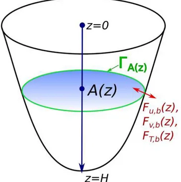
Figure 1. The schematic of a water body where 3-D thermodynamic and hydrodynamic equations are averaged at each horizontal cross section.
The needed closure is derived in subsequent parts of the paper: Section 3 recalls the reader the basics of mul-tilayer seiche models and derives mechanical energy conservation law, to be complied in finite-difference solutions implemented below; section 4 rewrites multilayer model for a specific case when only 1-st hori-zontal seiche mode exists and when horihori-zontally averaged velocities are coupled with averaged horihori-zontal pressure gradient in a closed equation set; analytical properties of reduced system are studied. Section 5 pro-vides theoretical grounds for coupling 1-D equations for horizontally averaged velocity to 1-st seiche mode equations and presents how this approach was implemented in existing structure of 1-D k −𝜖 model LAKE (Stepanenko et al., 2011, 2016). Section 6 is devoted to validation of the new version of LAKE model in idealized wind forcing scenarios and simulations of Lake Iseo (Italy), where the calculated seiche-caused fluctuations of temperature are compared to those measured in different locations of the lake. Conclusions summarize main findings of the paper and draw future perspectives of the new approach.
2. General 1-D Model Formulation for Enclosed Basins
Consider a water basin of arbitrary enclosed shape. Hereafter we assume that all functions and spatial domains are of sufficient smoothness so that all mathematical rules and theorems involved below are in force. First, introduce operation of averaging over the horizontal cross section of a water body A(z) (complete list of symbols is given in Appendix A, Table A1) for any scalar or vector variable𝑓:
̄ 𝑓 = A−1(
z)∫A(z)
𝑓dA′, (1)
where z is spatial coordinate along gravity (Figure 1). Applying this operation to temperature and horizontal momentum equations of an incompressible fluid yields (Stepanenko et al., 2016):
𝜕 ̄T 𝜕t = −𝒜T+ 1 A 𝜕 𝜕z ( A(𝜈T+𝜆m) 𝜕 ̄T 𝜕z ) − 1 A 𝜕ĀS 𝜕z + 1 A dA dz[Sb+FT,b(z)], (2) 𝜕 ̄u 𝜕t = −𝒜u− ( 1 𝜌 𝜕p 𝜕x ) + 1 A 𝜕 𝜕z ( A(𝜈 + 𝜈m) 𝜕𝜕z̄u ) + 1 A dA dzFu,b(z) + l̄v, (3)
𝜕̄v 𝜕t = −𝒜v− ( 1 𝜌 𝜕p 𝜕𝑦 ) + 1 A 𝜕 𝜕z ( A(𝜈 + 𝜈m) 𝜕𝜕z̄v ) + 1 A dA dzFv,b(z) − l̄u, (4)
where T is temperature; (u, v) =. uh is horizontal velocity;𝜆m, 𝜈 are coefficients of molecular con-ductivity and viscosity, respectively; 𝜈T, 𝜈m are coefficients of turbulent conductivity and viscosity;𝜌 is water density; l is Coriolis parameter; p is pressure; and S is kinematic flux of shortwave radiation; 𝒜𝑓 =. A−1(z)∫ΓA(z)𝑓(uh·n)dlΓis transport of𝑓 through the basin boundaries, carried out by inlets, outlets, and groundwater discharge (n is outer normal to the boundary of basin's horizontal cross-section ΓA(z)). Lower index “b” indicates the values of fluxes of respective variables at the boundary ΓA(z), that is, at the lake bottom of depth z. A satisfactory assumption usually used is ̄S(z) = Sb(z); that is, radiation flux is taken to be horizontally homogeneous at all depths. Reduced forms of the given system are solved in many 1-D lake models (Goudsmit et al., 2002; Fang & Stefan, 2009; Jöhnk & Umlauf, 2001; Tan & Zhuang, 2015; Zinoviev, 2014). Systems (2)–(4) are also solved in LAKE 2.0 model, where the mean horizontal pressure gradient is treated as barotropic gradient (Stepanenko et al., 2016; see details in subsequent sections).
Systems (2)–(4) do not contain vertical velocity, so that there is no need for additional equation for this variable. In more general case, when there is imbalance of inflows and outflows, mean vertical advection should be included. Mean vertical speed ̄w in this case may be found by averaging in horizontal the conti-nuity equation. Vertical momentum equation in lakes is well approximated by hydrostatic relation, which is used later in this paper in pressure gradient parameterization.
Two simple parameterizations can be used to compute bottom drag:
(Fu,b, Fv,b) =cb,linuh−linear drag, (5)
(Fu,b, Fv,b) =cb,quad|uh|uh−quadratic drag, (6) where cb,linand cb,quadare constant linear and quadratic drag coefficients, respectively.
This paper aims to develop a closure for the horizontal pressure gradient terms of systems (2)–(4) in a gen-eral, baroclinic, case when a water basin is stratified by density. This closure can be derived analytically when a basin is a parallelepiped [−Lx∕2, Lx∕2] × [−L𝑦∕2, L𝑦∕2] × [0, H]; then, A(z) = const, which signifi-cantly simplifies equations (2)–(4). Most of analytical derivations in subsequent sections are performed for this case. For simulations of Lake Iseo, a generalization of the closure to a case of arbitrary lake shape will be introduced.
3. Mulitlayer Model for Basins With Vertical Walls
This section reminds the reader the basics of multilayer models and presents a mechanical energy conser-vation law for multilayer fluid involving newly derived available potential energy.
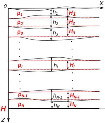
In a multilayer model the water body is composed of N layers of constant densities𝜌ithat are increasing with depth (𝜌i+1> 𝜌i); the thicknesses of these layers are supposed to deviate negligibly compared to reference values, hi=Hi+h′ i, ( |h′ i∕Hi| ≪ 1, ∑N i=1Hi=H )
(Figure 2). For each layer, the linearized equations for momentum (ui, vi)and mass conservation read (no summation on repeated indices is assumed) as follows:
𝜕ui 𝜕t = − 1 𝜌i 𝜕p′ i 𝜕x +lvi, (7) 𝜕vi 𝜕t = − 1 𝜌i 𝜕p′ i 𝜕𝑦 −lui, (8) 𝜕h′ i 𝜕t +Hi (𝜕u i 𝜕x + 𝜕vi 𝜕𝑦 ) =0, (9) p′ i=g N ∑ k=1 𝜌min(i,k)h′k, i = 1, N, (10)
Figure 2. The sketch of a multilayer model for 2-D basin.Hi—reference thickness ofith layer, the density ofith layer is
𝜌i,hiis an actual thickness evolving in time,hi=Hi+h′i(the schematic is adopted from Münnich et al., 1992). where g is acceleration due to gravity. Systems (7)–(10) are considered in a domain A of x-𝑦 plane and supplemented by conditions of impermeability at the lateral boundaries of each layer:
[
(ui, vi) ·n ]
ΓA=0, i = 1, N, (11)
with n standing for the outer normal to the boundary ΓAof A. It is likely that the first who considered the same kind of a system of coupled shallow water equations (for a case N = 3) was G. Csanady in his study of the coastal upwelling Csanady (1982). Later, Monismith (1985) and Münnich et al. (1992) applied the similar model for lakes. The criteria for validity of the two-layer model are given in Spigel (1978) and—in a case of geostrophic approximation—by J.Pedlosky Pedlosky (1979). According to R. Spiegel (Monismith, 1985; Spigel, 1978), these criteria may be expressed in terms of Richardson number Ri, Wedderburn number W, and the ratio of a basin width to internal Rossby radius (Kelvin number, Ke):
W=. g𝜖H 2 1 u2 ∗max(Lx, L𝑦) → ∞, (12) Ri=. g𝜖H1 u2 ∗ → ∞, (13) Ke=. lmin(Lx, L𝑦) (g𝜖H1)1∕2 → 0, (14)
where Lx, L𝑦are horizontal dimensions of a basin, H1is the thickness of the upper mixed layer, u∗is friction
velocity at the water surface,𝜖 = (𝜌2−𝜌1)∕𝜌2. Equation (12) is condition for smallness of layer thickness
deviations, that is, it justifies linearization. The limit (13) is a necessary condition for validity of hydrostatic approximation for small water bodies, that is, lakes with min(Lx, L𝑦)≪ LR(which is exactly the condition (14)). Note that the first and the last of given conditions contain lake size in a way that for the small water bodies they are fulfilled better. Moreover, W = ArRi, where Ar
.
= H1∕max(Lx, L𝑦)is the aspect ratio and
The key special cases of a linear multilayer model are single-layer (barotropic) model and a two-layer, simplest baroclinic, model. An important feature of the multilayer model is a mechanical energy conserva-tion law.
The kinetic energy of the fluid governed by (7)–(10) is defined as follows:
K =1 2 N ∑ i=1 Hi𝜌i∫ A ( u2 i+v 2 i ) dA′. (15)
Introduce a new variable
Ae= g 2 N ∑ i=1 Δ𝜌i ∫A (N ∑ k=i h′ k )2 dA′, (16)
where Δ𝜌1 = 𝜌1and Δ𝜌i = 𝜌i−𝜌i−1when i ≥ 2. Involving equations (7)–(10), the mechanical energy
conservation for the nondissipative system may be proven (see Text S1 in the supporting information) d(K + Ae)
dt =0. (17)
Variable Aeis an extension of the available gravitational potential energy derived for a two-layer liquid in Leonardi (2011). From (16) it is easily seen that the rest of systems (7)–(10) (ui, vi, h′
i = 0, i = 1, N) correspond to a minimal value Ae = 0. The mechanical law conservation given above will be taken into account when constructing a seiche parameterization and in numerical implementation of the latter. A bulk of observational evidence suggests that seiche modes with 1-st horizontal wavenumber carry the dominant part of internal wave energy (Horn et al., 1986; Kirillin et al., 2015; Lemmin et al., 2005; Marchenko & Morozov, 2016; Rueda & Schladow, 2002; Roget et al., 2017). Thus, as a first approximation, only these modes are taken into account in a seiche parameterization. The spatial structure of 1-st horizontal mode, being and eigenfunction of the problems (7)–(11), depends on a form of the domain A and on whether l = 0 or l≠ 0 (Csanady, 1967; Rao, 1966). In rectangular domain A with no rotation eigenfunctions are sines and cosines. A version of multilayer model for 1-st horizontal mode based on harmonic functions is given in the following section.
4. Multilayer Seiche Model for the 1-st Horizontal Mode
This section derives a new approximate set of dynamic equations for horizontally averaged velocity and pressure gradient from a multilayer model system, assuming 1-st horizontal mode only, and examines its analytical properties by comparing to classical solutions. Horizontal averaging is performed in order to get additional equations for velocities and pressure gradient involved in 1-D model.
4.1. Derivation of the Model 4.1.1. Two-Dimensional Basin
Equations 7–(10) for a two-dimensional channel [−L∕2, L∕2] × [0, H] without rotation reduce to (Münnich et al., 1992): 𝜕ui 𝜕t = − 1 𝜌i 𝜕p′ i 𝜕x, (18) 𝜕h′ i 𝜕t +Hi 𝜕ui 𝜕x =0, (19) p′ i=g N ∑ k=1 𝜌min(i,k)h′k, i = 1, N. (20) Now, for any variable𝑓 we introduce the horizontal average ̄𝑓 = 1∕L ∫−L∕L∕22𝑓dx, the average over the left part of domain ̄𝑓1=2∕L∫0
−L∕2𝑓dx and the average over the right part ̄𝑓
2=2∕L∫L∕2
0 𝑓dx. Here, we located
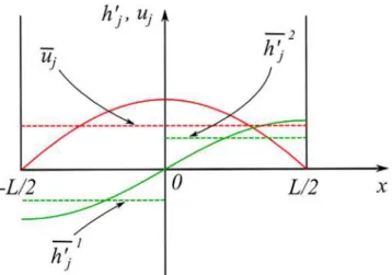
Figure 3. The 1-st horizontal Fourier mode of speedu𝑗and thickness deviationh′
𝑗of𝑗th constant density layer (solid
lines):u𝑗∝cos(𝜋x∕L),h′𝑗∝sin(𝜋x∕L). Due to hydrostatic approximation,p′𝑗∝sin(𝜋x∕L). Dashed lines represent averaged quantities defined in text.
ui∝cos(𝜋x∕L), p′i∝sin(𝜋x∕L), i =1, N, (21) where p′
iis deviation of pressure from its value at the rest of a liquid. Then, averaging (18)–(20) yields the following: dui dt = − 1 L𝜌i ( p′ i|x=+L∕2−p′i|x=−L∕2 ) = − 𝜋 2L𝜌i ( p′ i 2 −p′ i 1) , (22) dh′ i 2 dt = − dh′ i 1 dt = 2Hi L ui|x=0= 𝜋Hi L ui, (23) p′ i 𝑗 =g N ∑ k=1 𝜌min(i,k)h′k 𝑗 , 𝑗 = 1, 2, i = 1, N. (24)
Eliminating pressure in the above system and introducing a mean thickness gradient Δh′
k=h ′ k 2 −h′ k 1 , we finally get a closed equation set:
dui dt = − 𝜋g 2L𝜌i N ∑ k=1 𝜌min(i,k)Δh′k, (25) dΔh′ i dt = 2𝜋Hi L ui, i = 1, N. (26)
We may note that extension of the approach presented here to an arbitrary number of horizontal modes is possible but is postponed for future studies; interestingly, it would involve only modes with odd numbers, as horizontal harmonic modes with even numbers have zero horizontal average and thus they do not contribute to horizontally averaged velocity.
4.1.2. Three-Dimensional Basin
Now, consider equations 7–(10) in 3-D water body [−Lx∕2, Lx∕2] × [−L𝑦∕2, L𝑦∕2] × [0, H] without rotation, that is, l = 0. The 1-st Fourier mode in this case reads as follows:
ui=ui10cos ( 𝜋x Lx ) +ui11cos ( 𝜋x Lx ) sin ( 𝜋𝑦 L𝑦 ) , (27) vi=vi 01cos ( 𝜋𝑦 L𝑦 ) +vi 11sin ( 𝜋x Lx ) cos ( 𝜋𝑦 L𝑦 ) , (28)
hi=hi10sin ( 𝜋x Lx ) +hi01sin ( 𝜋𝑦 L𝑦 ) +hi11sin ( 𝜋x Lx ) sin ( 𝜋𝑦 L𝑦 ) , (29)
Adopting the same derivation technique as used above for the 2-D basin yields dui dt = − 𝜋g 2Lx𝜌i N ∑ k=1 𝜌min(i,k)Δxh′k, (30) dvi dt = − 𝜋g 2L𝑦𝜌i N ∑ k=1 𝜌min(i,k)Δ𝑦h′k, (31) dΔxh′i dt = 2𝜋Hi Lx ui, (32) dΔ𝑦h′ i dt = 2𝜋Hi L𝑦 vi, i = 1, N. (33) Here, Δxh′ i=h ′ i x2 −h′ i x1 , h′ i x1 = 2 LxL𝑦∫ 0 −Lx∕2∫ L𝑦∕2 −L𝑦∕2 h′ id𝑦dx, h′ i x2 = 2 LxL𝑦∫ Lx∕2 0 ∫ L𝑦∕2 −L𝑦∕2 h′id𝑦dx,
and analogous operators in𝑦 direction are defined accordingly. Note that equations (30) and (32), on the one hand, and (31) and (33) on the other are independent equation subsets. Now, the effect of Earth rotation can be formally added as extra terms +lviand −luion the right-hand side (r.h.s.) of (30) and (31), respectively, to get dui dt = − 𝜋g 2Lx𝜌i N ∑ k=1 𝜌min(i,k)Δxh′k+lvi, (34) dvi dt = − 𝜋g 2L𝑦𝜌i N ∑ k=1 𝜌min(i,k)Δ𝑦h′k−lui. (35) This is not an analytically exact way of including rotation. We would have retained Coriolis force in (7)–(10) and performed analytical derivation using (27)–(29) to get an equation set analogous to (30)–(33) for the 1-st horizontal mode but including rotation. However, when including Coriolis force, harmonic functions do not more represent the horizontal structure of single modes (including 1-st mode), that is, formally, they are not eigenfunctions of the equation set. To avoid using complicated eigenfunctions for rotating rectangular basin Rao (1966), we formally add Coriolis terms to r.h.s. of (34) and (35). As it is not justified rigorously, we analyze the properties of the resulting system below.
First, systems (34) and (35) and (32) and (33) provide a mechanical energy conservation law Ae+K=const, where K =1 2 N ∑ i=1 Hi𝜌iLxL𝑦(̄u2 i+̄v 2 i ) , (36) Ae= gLxL𝑦 8 N ∑ i=1 Δ𝜌i ⎡ ⎢ ⎢ ⎣ (N ∑ k=i Δxh′ k )2 + (N ∑ k=i Δ𝑦h′ k )2⎤ ⎥ ⎥ ⎦, (37)
which is a special case of a general law (17). It can be easily proven that available potential energy Aedefined here is zero when and only when Δxh′k= Δ𝑦h
′
k=0, k = 1, N, so that all isosteric surfaces are horizontal. Then, the oscillatory solutions of the set (34) and (35) and (32) and (33) can be compared to other analytical solutions available in literature. The case where inertia-gravity waves in an enclosed basin are studied in details is that for cylindrical basin in Csanady (1967). Thus, using results of Csanady (1967) would reveal the joint effect of two deficiencies in (34) and (35): (i) formally adding Coriolis force to the system derived without rotation and (ii) applying the system derived for rectangular basin to cylindrical basin. One more important property of system (34) and (35) and (32) and (33) is that when horizontal dimensions Lx and
L𝑦much exceed Rossby deformation radius, pressure gradient force vanishes, leading to classical rotating boundary layer equations. Both aspects mentioned here are covered in section 4.2.2.
4.2. Analytical Evaluation of the 1-st Seiche Mode Model 4.2.1. Two-dimensional Basin With No Rotation
4.2.1.1. Oscillation Frequencies
From the system of 2N equations (25) and (26) one derives N equations for averaged velocities: d2u i dt2 = − 𝜋2g L2𝜌 i N ∑ k=1 𝜌min(i,k)Hkuk. (38) This system is a special case of a more general set (Münnich et al., 1992):
𝜕2u i 𝜕t2 = g 𝜌i N ∑ k=1 𝜌min(i,k)Hk 𝜕2u k 𝜕x2. (39)
It is easily seen that equation (38) follows when substituting the 1-st modes (21) to (39). Hence, the frequen-cies of internal oscillations of systems (25) and (26) coincide to those of the 1-st mode in the set (39). The latter, in turn, are shown to be well consistent with maxima in observed spectra of temperature in thermo-cline (Münnich et al., 1992). The oscillation frequencies𝜔 are√|𝜆|, 𝜆 < 0, 𝜆 being eigenvalues of a matrix
Aof the r.h.s. in (38) and can be found as solutions of the eigenvalue problem:
det (A −𝜆I) = 0, (40)
where I is a unit matrix.
4.2.1.2. Wedderburn Number Criterion
Now consider a stationary position of the internal surface in a two-layer fluid imposed to a constant wind stress. Systems (25) and (26) in a stationary case and N = 2, supplemented by wind stress on the top layer, yield 0 = u 2 ∗ H1 −𝜋g 2L [ Δxh′ 1+ Δxh′2 ] , (41) 0 = − 𝜋g 2L𝜌2 [ 𝜌1Δxh′1+𝜌2Δxh′2 ] , (42) u1=u2=0. (43)
Thence, after some algebra, we get
Δ H1 = u 2 ∗L 2g′H2 1 = 1 2W, (44) where Δ = |||h′
2|x=+L∕2||| = |||h′2|x=−L∕2|||is an absolute value of vertical displacement of the interface from
horizontal position at the edges of a basin, W ∼ Fr−1is a Wedderburn number. Therefore, the condition for the interface to reach the surface reads
W ≤ 1
2 (45)
that agrees to existing estimates providing values for this threshold in a range 0.5–1 (Imberger & Hamblin, 1982; Kirillin & Shatwell, 2016; Shintani et al., 2010).
4.2.2. The 3-D Basin With Rotation
Here we will examine the two cases of the full system (34) and (35) and (32) and (33) that are tractable analytically: barotropic fluid (N = 1) and two-layer baroclinic fluid (N = 2).
4.2.2.1. Barotropic Case
Purely barotropic motions in a system (34) and (35) and (32) and (33) are attained when N = 1. Substituting harmonic solution (𝑓 ∼ exp(̄ζ𝜔t), 𝑓 = u1, v1, … , ̄ζ =
√
−1) in the system yields:
𝜔2=1 2 [( 𝜔2 gx+𝜔 2 g𝑦+l2 ) ±√(𝜔2 gx+𝜔2g𝑦+l2 )2 −4𝜔2 gx𝜔2g𝑦 ] , (46) where𝜔gx =𝜋L−1x √ gH1, 𝜔g𝑦=𝜋L−1𝑦 √
gH1are frequencies of surface gravitational modes along respective
horizontal axes, and𝜔2is always positive.
The frequencies of gravitational and inertial oscillations are special cases of (46). Indeed, if𝜔gx ≫ l or
𝜔g𝑦≫ l, then (46) provides
𝜔 = ±𝜔gx, ±𝜔g𝑦 (47)
that are frequencies of oscillations in (34) and (35) and (32) and (33), independent in two horizontal direc-tions, if setting l = 0. The conditions𝜔gx ≫ l or 𝜔g𝑦≫ l are equivalent to Lx∕LR≪ 𝜋 or L𝑦∕LR≪ 𝜋, where
LR= √
gH1∕l– barotropic Rossby radius of deformation. This means that, in order to neglect the effects of
inertial motion caused by Earth rotation, it is sufficient that at least in one horizontal direction the water body size is much less than LRthat is consistent with analytical solutions for Kelvin and Poincaré waves in rectangular basins and channels (Gill, 1982; Taylor, 1921). For instance, Kelvin waves in an infinite channel of constant depth filled with homogeneous fluid reduce to gravitational modes if the channel width is much less than LR(Hutter, 1984). Inertial oscillations in (46) are achieved in a limit of large Lx∕LR, L𝑦∕LR. In the following, it is convenient to distinguish between the modes with|𝜔| > l (Poincaré modes) and those with|𝜔| < l (Kelvin modes). This terminology is exploited, for example, by A.Defant Defant (1961) and then by G.T.Csanady Csanady (1967). It is straightforward to show that choosing the sign “plus” in (46) leads to two roots|𝜔+,1,2| > l, that is, Poincaré mode. On the contrary, the frequencies 𝜔−,1,2, resulting from using “minus” sign in (46), may be either larger or smaller in absolute value than the inertial frequency. For simplicity consider a basin with rectangular horizontal cross section, Lx=L𝑦=L, so that𝜔gx=𝜔g𝑦=𝜔g. In this case,|𝜔−,1,2| < l under condition 𝜔2g< 2l2, and otherwise|𝜔−,1,2| > l. Thus, the condition for existence of Kelvin mode is 𝜔2 g< 2l 2 or L LR > √ 2𝜋 2 ≈2.22. (48)
The ratio L∕LRis often referred to as Kelvin number. Note that
|𝜔−| → 0 and |𝜔+| → l if L∕LR→ ∞. (49)
that is, when the lake size much exceeds the Rossby radius, the Kelvin mode turns to a stationary one, while a Poincaré mode transforms to an inertial oscillation. The stationarity of Kelvin mode in a limit of very vast water basin means that given the fixed phase speed of this wave type√gHGill (1982) increase of basin size decreases the angular velocity of margin-bound ridges and troughs in respect to basin center. Reduction of Poincaré modes to inertial oscillations also conforms with classical analysis of shallow water equations in a rotating system of reference Gill (1982).
Since the model (34) and (35) and (32) and (33) has been derived for rectangular basin the question emerges how the properties of its solutions discussed above correspond to those taking place in basins of other shapes. Analytical solution for barotropic inertial-gravitational waves in circular lake is given in Csanady (1967) and Lamb (1932). Its analysis leads to criterium for existence of first Kelvin mode:
2r0
LR
which is close to condition (48) (r0standing for lake radius). At large r0∕LRthe frequency of 1-st Kelvin mode in circular basin is𝜔 ∼ −lLR∕r0, that is, approaches zero. This limit also agrees to the first limit of (49). The
minimal frequency of Poincaré modes in circular domain does not significantly exceed l Lamb (1932) that conforms to second limit in (49).
4.2.2.2. Two-Layer Baroclinic Case
The two-layer problem (34) and (35) and (32) and (33) is reduced to two independent single-layer problems by an elegant introduction of new variables, proposed by G.Veronis Veronis (1956):
u∗iH∗i= (1 −𝛽i)u1H1+u2H2, (51)
v∗iH∗i= (1 −𝛽i)v1H1+v2H2, (52)
h′
∗i= (1 −𝛽i)h′1+h′2, i =1, 2, (53)
where𝛽i, i = 1, 2 are roots of the Stokes equation:
H1𝛽2−𝛽(H1+H2) +𝜖H2=0, (54) 𝛽1,2= H1+H2 2H1 ( 1 ± √ 1 − 4𝜖H1H2 (H1+H2)2 ) , (55)
H∗i=𝜖H2∕𝛽i, and𝜖 = (𝜌1−𝜌2)∕𝜌2. Taken into account the smallness of𝜖, it can be shown that
𝛽1= H1+H2 H1 +O(𝜖), H∗1≈ 𝜖H1H2 H1+H2 , (56) 𝛽2= 𝜖H2 H1+H2 +O(𝜖2), H ∗2≈H1+H2, (57)
that is, the single-layer system (34) and (35) and (32) and (33) written in respect to u∗1, v∗1, h∗1, H∗1
describes baroclinic motions and that for u∗2, v∗2, h∗2, H∗2barotropic ones. Therefore, the analysis
of frequencies performed in previous section for single-layer system literally holds for the two solutions of two-layer system (baroclinic, i = 1 and barotropic, i = 2), with formal substitution H1 → 𝜖H1H2
H1+H2 and
H1→ H1+H2, respectively.
5. Coupling 1-D Lake Model to a Multilayer Seiche Model
5.1. Theoretical Arguments and Final Equation Set
A remarkable feature of a system (34) and (35) and (32) and (33) is that it links horizontally averaged veloc-ity components to averaged pressure gradient. This suggests to use equations 34 and (35) and (32) and (33) for closure of a target 1-D system (2)–(4) for a case of rectangular cross section of a water body, constant with depth (A(z) =const). However, equations (2)–(4) are differential in coordinate z, while in a multilayer model (34) and (35) and (32) and (33) the vertical profiles of thermodynamic and hydrodynamic variables are assumed piecewise constant. In this paper, a validity of coupling of two systems is not proved mathemat-ically; rather a physical rationale is presented, so that the resulting method for calculation of the pressure gradient terms in 1-D model is correct to refer to as parameterization.
In a continuous vertical density profile𝜌(z) = ΦEOS[ ̄T(z)](where ΦEOSis an equation of state chosen), cal-culated by 1-D model, we identify intervals [zi, zi+1), Hi = zi+1−zi, i = 1, N, so that in each interval density does not vary significantly (an algorithm for identification of those intervals is given in Text S3 of the supporting information) and introduce mean densities ̂𝜌i
.
=H−1
i ∫ zi+1
zi 𝜌(z)dz. Given that in 1-D model all variables are given at a numerical grid, these “constant density layers” are obtained by grouping the 1-D model numerical layers (Figure 4). Then, we define variables Δxh′
i, Δ𝑦h′i, and to calculate them via formu-las (32) and (33), the layer-wise averaged velocity components from 1-D model (̂ui, ̂vi) = Hi−1∫
zi+1
zi (̄u, ̄v)dz are involved. The horizontally averaged pressure gradient given by Δxh′i, Δ𝑦h
′
i, i = 1, N, is the piece-wise constant function of z, with a single value inside each interval [zi, zi+1), and it is now introduced into
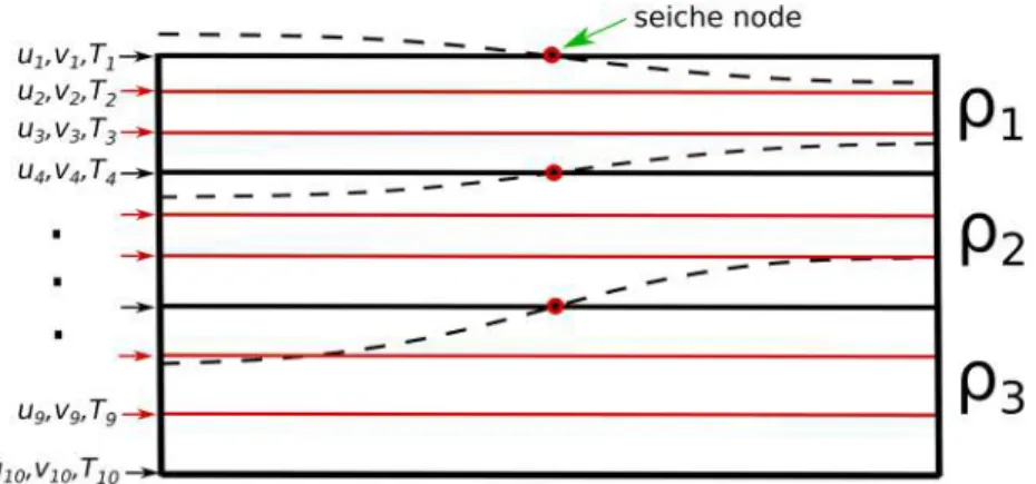
Figure 4. Levels of 1-D lake model numerical grid (red lines) and constant density layers (with margins denoted by black bold lines) used in horizontal pressure gradient parameterization. Dashed black lines represent 1-st horizontal mode deviations of layers' interfaces.
𝜕 ̄u 𝜕t − 𝜕𝜕z(𝜈 + 𝜈m) 𝜕𝜕z̄u−l̄v = − 𝜋g 2Lx̂𝜌i N ∑ k=1 ̂𝜌min(i,k)Δxh′k, i ∶ z ∈ [zi, zi+1), (58) 𝜕̄v 𝜕t − 𝜕𝜕z(𝜈 + 𝜈m) 𝜕𝜕z̄v+l̄u = − 𝜋g 2L𝑦̂𝜌i N ∑ k=1 ̂𝜌min(i,k)Δ𝑦h′k, i ∶ z ∈ [zi, zi+1), (59) dΔxh′ i dt = 2𝜋Hi Lx ̂ui, i = 1, N, (60) dΔ𝑦h′ i dt = 2𝜋Hi L𝑦 ̂vi, i = 1, N, (61) (̂ui, ̂vi) =H−1 i ∫ zi+1 zi (̄u, ̄v)dz, i = 1, N. (62)
This system may be solved by time-splitting finite-difference scheme in two stages:
1. Calculation of tendencies of velocity components caused by only pressure gradient terms coupled to a performing one time step of equations (60)–(62) by Crank-Nicolson scheme. This scheme ensures con-servation of mechanical energy Ae+K( (36)–(37)). Implicit scheme leads to solution of linear equation set with dense matrix, which we solve by a direct method; with typical values N ≈ 2 … 10 the CPU time for this solution is small compared to total CPU time of the 1-D lake model (2–4%).
2. Update of velocity components due to vertical viscosity and Coriolis terms. Here, Crank-Nicolson scheme is used as well, with central differences for spatial derivatives.
Note that the method used here to couple a system (34) and (35) and (32) and (33) to a 1-D model equation set is an extension of approach suggested by Svensson (1978), that is, the latter is equivalent to ours if N = 1, that is, when only the barotropic pressure gradient is considered.
The drawback of a system (58) and (62) is that vertical distribution of horizontal pressure gradient is assumed stepwise. This leads to emergence of large velocity shear at the interfaces of constant density layers zi, which in turn produces high TKE and turbulent viscosity/diffusivity in k −𝜖 closure at those depths. The remedy we propose is to replace the r.h.s. of (58) and (59), which is constant in each ith layer, by smooth functions of z, Fp,x,i(z), and Fp,𝑦,i(z), with the vertical averages equal to original terms:
H−1 i ∫ zi+1 zi Fp,x,i(z)dz = − 𝜋g 2Lx̂𝜌i N ∑ k=1 ̂𝜌min(i,k)Δxh′k, i = 1, N, (63)
and equation for Fp,𝑦,ihas the similar form. The second condition for functions Fp,x,iand Fp,𝑦,iwould be continuity at depths zi. These requirements allow to define Fp,x,iand Fp,𝑦,ias unique quadratic functions of
zin each constant density layer. Moreover, it is straightforward to show that neglecting viscosity terms in (58) and (59) both stepwise and smooth representation of pressure gradient force lead to identical equations in respect to layer-averaged velocities (̂ui, ̂vi)(one should just integrate (58) and (59) in vertical in each ith layer).
In lakes, density stratification significantly evolves on a seasonal timescale. It means, that in the model, the number and location of constant density layers approximating current density profile should change (“relayer”) at some instants, and layer-linked variables Δxh′i, Δ𝑦h
′
ishould be reset after each such a change for a new set of layers. It is done as follows. If a criterium for relayering is matched (see Text S3), Δxh′
i, Δ𝑦h′i are first evenly distributed between numerical layers comprising each old constant density layer (Figure 4) and then are summed up to get values Δxh′
i, Δ𝑦h′ifor the new constant density layers.
Since in the new model presented above not only vertical structure of a current but also the 1-st horizontal mode are explicitly reproduced, the model may be termed as 112-dimensional. The number of vertical seiche modes resolved in the model is the number of constant density layers N, for example, when N = 3 the model simulates dynamics of modes H1V0, H1V1, and H1V2.
In essence, the physical effect of introducing pressure gradient into 1-D lake model is as follows. Basin-scale (1-st mode) pressure gradient affects the basin-scale (basin-averaged) velocity and thus controls the vertical velocity shear which acts in a TKE production term in k −𝜖 closure. Hence, the pressure gradient parame-terization ultimately modifies vertical turbulent fluxes and the surface mixed-layer depth. In turn, this leads to changes in vertical distribution of temperature and solutes. The latter effect is not covered in this paper and is postponed for future research.
An extension of pressure gradient parameterization developed above to a case of arbitrary hypsometric curve
A(z)is given in Text S2. In this case, horizontal dimensions of constant density layers are nonincreasing with depth, Lx,i+1≤ Lx,i, L𝑦,i+1≤ L𝑦,i. The extension to (58)–(62) is based on representing the horizontal struc-ture of speed and thickness in each constant density layer by 1-st harmonic mode (Figure S1), so that (60) and (61) hold and introducing new pressure gradient transfer coefficients in r.h.s. of (58) and (59) ensuring mechanical energy conservation law with appropriate definition of available potential energy. Represent-ing h′
iby 1-st Fourier mode (as it shown at Figure 3) in this case still well corresponds to vertical velocity pattern of analytically derived modes (see H1 modes found in Fricker and Nepf (2000) for a basin with slop-ing bottom indicatslop-ing upward (h′
i> 0) and downward (h
′
i< 0) motions at opposite bottom sides), whereas assuming horizontal speed vanishing at sidewalls is less realistic now, as the real bottom is very different from vertical wall. Nevertheless, our simulations show that the vertical structure of horizontally averaged velocity (with surface along-wind current and counter-current in the bottom of mixed layer) is qualitatively reproduced in such a framework as well, and the magnitude of currents are controlled by mechanical energy conservation.
5.2. Reconstructing Temperature Series in Selected Lake Locations
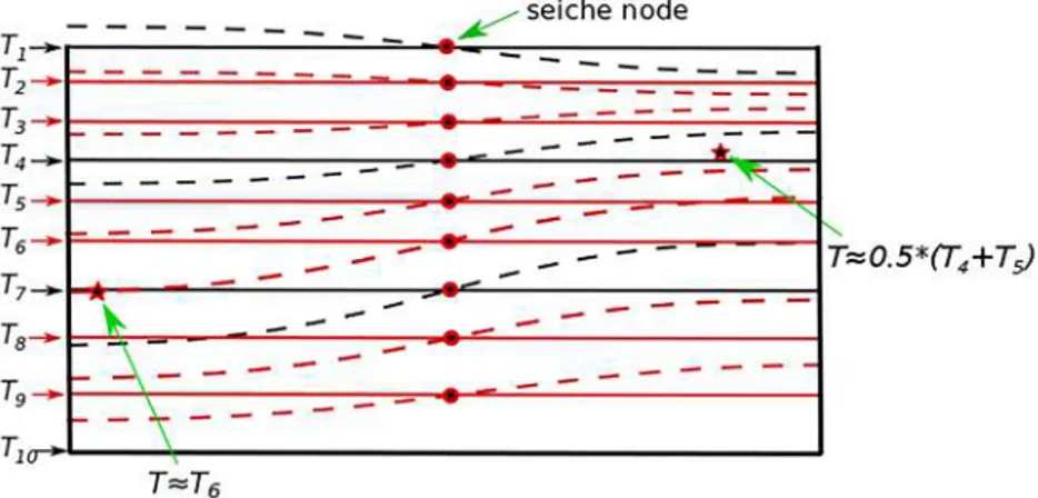
Using the parameterization of horizontal pressure gradient developed above, it is possible to reproduce seiche-induced oscillations of thermodynamic variables (e.g., temperature) at each location of a water basin. To do this, we assume that constant-value surfaces of water physical properties, being horizontal and coin-ciding with levels of 1-D model numerical grid at rest, follow the motion of boundaries of constant density layers (Figure 5). In other words, each thermodynamic variable has the same horizontal structure as the 1-st mode of h′, because it is advected by vertical velocity governed by h′. Thus, given values of Δ
xh′iand Δ𝑦h
′
i, the position of isosurfaces “carrying” physical properties of the 1-D model numerical levels is reconstructed, and then, for each location (x, 𝑦, z) the thermodynamic variable is interpolated between two adjacent isosurfaces. 5.3. LAKE Model
The 1-D thermodynamic, hydrodynamic, and biogeochemical model LAKE (Stepanenko et al., 2011, 2016) simulates vertical transport of heat in a basin taking into account volumetric absorption of shortwave radi-ation in water, ice, snow, and underlying sediments. The model equradi-ations are formulated in terms of water properties averaged over a lake's horizontal cross section, thus introducing into the model fluxes of momen-tum, heat, and dissolved gases through a sloping bottom surface (see equations (2)–(4)). In water, k −𝜖 parameterization for turbulent fluxes is used. In momentum equations, barotropic pressure gradient is
Figure 5. The sketch for reconstruction of seiche-induced oscillations of thermodynamic variableTin two selected points. Black bold and dashed lines, bold red lines are the same as in Figure 4. The levels of numerical grid of 1-D lake model are treated as isosurfaces of valuesTi, respectively, at rest. Dashed red lines are the same isosurfaces perturbed following motion of boundaries of constant density layers. Two asterisks denote locations where time series of a thermodynamic variable are reconstructed as linear interpolation between values ofTat adjacent isosurfaces.
accounted for Stepanenko et al. (2016). Water density is computed by equation of state from McCutcheon et al. (1993). In ice and snow, a coupled transport of heat and liquid water is reproduced (Stepanenko et al., 2019). In bottom sediments, phase transitions of water affect thermal regime. The model simulates vertical diffusion of dissolved CO2, CH4, and O2, as well as bubble flux of these gases, methane production, and
oxi-dation, photosynthesis, and biogeochemical processes consuming oxygen and releasing carbon dioxide. The fluxes of heat, water, and momentum to the atmosphere are computed via Monin-Obukhov similarity the-ory including universal functions of stability from Businger et al. (1971) and Paulson (1970). The model has been extensively verified at a number of lakes covering a wide range of climate conditions, for example, in a framework of LakeMIP project (Lake Model Intercomparison Project, Stepanenko et al., 2013, 2014; Thiery et al., 2014).
A generalized form of horizontal pressure gradient parameterization for A(z) decreasing with depth (Text S2) is introduced into the LAKE model. Characteristics of barotropic and baroclinic oscillations arising in the new version of the model for a case of 2-D nonrotating basin have been successfully tested versus analytical eigenvalue problem solutions in Stepanenko (2018). Below, the new version of LAKE model is applied to Lake Iseo.
6. Validation of the Model for Lake Iseo
6.1. The Site and Measurements
Lake Iseo is a 256 m deep and 60.9 km2large Italian lake, which represents well the features of other large
lakes located south of the Alps. During the second half of the twentieth century the deep water recirculation has been insufficient and the lake underwent a dramatic deterioration of water quality. Accordingly, a strong interest of the scientific community is to understand the mechanisms controlling the lake's circulation and to foresee the deep renewal evolution under climate change scenarios.
At this purpose, 1-D simulations were previously developed (Valerio et al., 2015), showing a reduced deep mixing favored by the increased air temperature and the modified discharge regime. Though, starting from Valerio et al. (2012), several experimental and numerical studies have shown the hydrodynamics of this lake to be dominated by basin-scale internal waves, featuring large and periodic oscillation both in the layers around the thermocline and deeper around the chemocline. The structure of the wind field was seen to favor the excitation of a first horizontal mode structure. Accordingly, a better long term modeling could profit from a proper parameterization of these oscillatory motions in the 1-D numerical schemes.
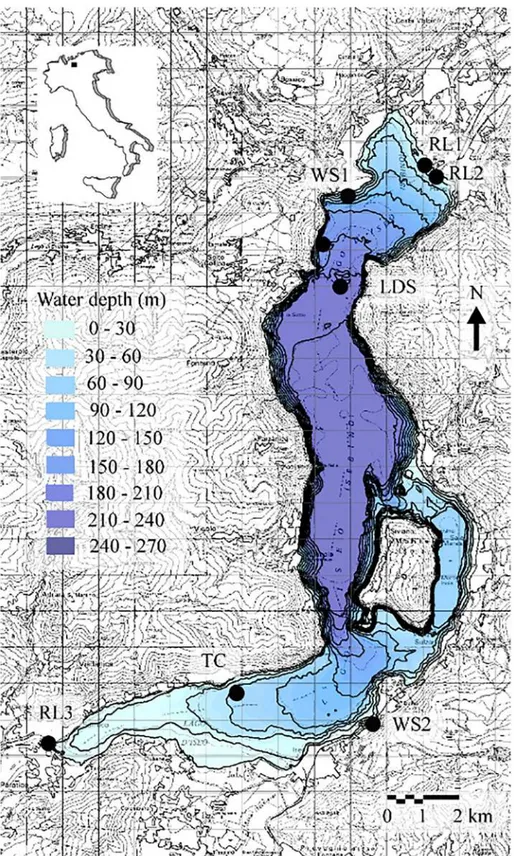
Starting from 2009, a network of gauging stations has been set up on Lake Iseo, providing water temperature and meteorological data suitable for model calibration. A floating station was moored in the northern part of the lake (LDS in Figure 6), measuring the main thermal, radiative, and mechanical fluxes on the lake surface. The temperature of the first 50 m of the water column was monitored with ±0.01◦C accuracy by
Figure 6. Lake Iseo, with bathymetry and observation stations. Details of the deployment of the measurement stations are described in Pilotti et al. (2013).
two submerged thermistor chains (LDS and TC in Figure 6) to quantify the temporal and spatial features of the main internal waves modes. Two additional wind stations (WS1 and WS2 in Figure 6) were installed to account for the spatial variability of the wind field. Finally, inflow and outflow discharges and temperature are measured at the mouth of the two main inflows (Oglio River RL1 in Figure 6 and Canale Industriale RL2 in Figure 6) and at the outflow (Oglio river RL3 in Figure 6).
The main feature of the lake shape is a presence of large island, and this invalidates assumption made in 1-D model that the horizontal cross section of a water body is simply connected; nevertheless, the dominance of modes with 1-st horizontal number revealed in studies of Lake Iseo mentioned above and the availability of temperature measurements in thermocline representing antinodes of 1-st horizontal modes makes the lake a suitable object for the model validation. Moreover, Rossby radius of deformation LR=NgH∕lis of an order of 10 km, when using 2011 year summertime vertically averaged values of Brunt-Väisälä frequency Ng (8 × 10⁻³ s−1) and the lake average depth 124 m; this means that Kelvin number based on the lake width
2.2 km is ≈0.2, and gravitational mechanism of oscillations dominates over the inertial one. This makes important the use of horizontal pressured gradient parameterization developed in this study.
6.2. The Model Setup
For the model validation a period 18 June to 10 October 2011 was chosen during which seiche oscilla-tions in the lake were clearly observed. In the late part of the period an abrupt change of lake stratification occurred (see below), which allows to test the model performance when the number and location of constant density layers alter significantly. In the model, the hypsometric function A(z) was set following measured bathymetry as shown in Figure 6. To specify Lx(z)and L𝑦(z), the horizontal aspect ratio of the water body was assumed constant, 0.15, at all depths, according to characteristic dimensions of the lake surface. Then, Lx(z)
and L𝑦(z)were computed from A(z) using approximation of the lake's horizontal cross section by rectangle. Thus, the lake surface had dimensions 20.1 km × 3 km. The depth of the water column was chosen 250 m. In numerical scheme, this depth was split in 200 layers, which were contracting toward the upper surface. Five soil columns originating from different depths were used to simulate heat exchange of Iseo Lake with the sloping bottom (Stepanenko et al., 2016). Two series of experiments have been performed, where the bottom friction was described by linear and quadratic law. In both cases, the bottom drag coefficient was the only parameter calibrated in the model to get the amplitude of seiche oscillations close to observed. Extinc-tion coefficient of shortwave radiaExtinc-tion was assumed constant, that is, the average of measured values, 0.33 m−1. In the equation for temperature (see term𝒜
Tin (2)), the heat advection by two inflows (Oglio River RL1 and Canale Industriale RL2) and one outflow (Oglio river RL3) was taken into account, given their measured discharges and temperatures. The background diffusivity in thermocline was parameterized as a function of Brunt-Väisälä frequency following Hondzo and Stefan (1993) and calibrated to match vertical temperature profile in this layer. Time step of numerical scheme was set to 10 s, bounded from above by using highly nonlinear k −𝜖 closure.
The number and locations of constant density layers in pressure gradient parameterization were updated at each time step of the model from current vertical density distribution as elaborated in section 5.1. The number of layers varied from 2 to 4 with the most frequent value of 3.
The initial profile of temperature was set from measurements at LDS station, as TC station did not provide temperature in the upper mixed layer. The model was forced by the hourly time series of shortwave and net radiation, pressure, air temperature, and humidity measured above the lake surface at LDS. Following the indications by Valerio et al. (2017), it was also forced by a uniform wind field having the same power as the spatially varying one and which was obtained by the spatial interpolation of the data measured at wind stations LDS, WS1, and WS2. The wind speed demonstrated distinct diurnal periodicity (not shown) characteristic of mountain-valley circulation.
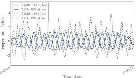
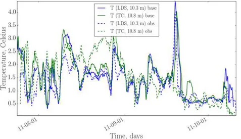
For comparison with model results, the data of two thermistor chains located at LDS and TC points (Figure 6) were used. At each point, the series from three depths were selected: 10.3, 14.8, 19.8 and m (LDS) and 10.8, 14.8, and 19.8 m (TC). These depths correspond to upper, middle, and deep thermocline, respectively (Figure 7) and represent different amplitude of vertical water movement. The LDS and TC points in the simulated lake are assumed to locate 7 km north and 8.5 km south from lake surface center, respectively. In order to assess the model capability to reproduce seiche dynamics, seiche-induced temperature fluctuations were derived by subtracting from measured and simulated temperature series the same series averaged by
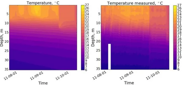
Figure 7. Temperature distribution over depth and time, modeled (left) and observed (right). Observed time series are averaged between series at LDS and TC stations. All data are smoothed by running mean with 1 day window.
running mean with 24-hr window (the period of dominant seiche motions in the lake):
T∗=T − ̃T, (64) ̃T(t) .= 1 t+−t− ∫ t+ t− Tdt′, (65) t+=min(t1, t + tav∕2), (66) t−=max(t0, t − tav∕2), (67)
where (t0, t1)is time interval of temperature series, tav = 24hr. Hereafter, series T∗ are referred to as
seiche oscillations. The temporal evolution of seiche magnitude is diagnosed as running root-mean-square deviation of seiche oscillations:
𝜎(T∗) = [ ̃ (T∗− ̃T∗)2 ]1∕2 . (68)
6.3. Results and Discussion
The model generally well reproduces the temperature distribution over time and depth (Figure 7; both sim-ulation and observation data were smoothed by 24-hr running average to highlight seasonal and synoptic variability of water temperature). The surface temperature is overestimated on average by 0.35◦C. This sys-tematic shift increases by ≈ 1◦C when heat advection by inflows and outflow is switched off. The seasonal surface mixed-layer depth deepening is captured by the model. According to observations, the isotherms in thermocline propagate slowly downward, the similar behavior observed in simulation results. When background diffusivity switched off in the model, only molecular heat conductance acts in metalimnion, and isotherms stay almost horizontal throughout simulation (not shown). This indicates to importance of background heat conductance extra to molecular which is not captured by standard k −𝜖 closure.
On 19 September 2011, a strong wind event occurs, leading to abrupt weakening of stratification and cool-ing the surface layer. The model and observations react differently: In the simulated temperature profile, the mixed layer deepens, thermocline staying almost “intact,” whereas the lower boundary of the observed thermocline significantly moves down. The resulting difference in stratification has a consequence on simulations of seiches (see below).
Calibration of linear bottom drag coefficient cb,linin LAKE model to match the observed amplitude of tem-perature oscillations in selected points resulted in a value 4 ×10⁻³m/s. In Valerio et al. (2012), a value 10−2
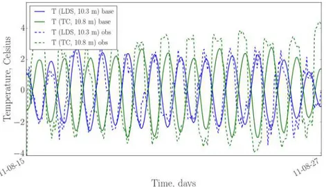
Figure 8. An excerpt of water temperature seiche oscillationsT∗, measured (“obs”) and simulated (“base”) in TC (10.8 m) and LDS (10.3 m) locations.
equations where spatial patterns of different horizontal modes are explicitly found as eigenvectors Shimizu and Imberger (2008) of linear equation set. Given the difference of models and data sets they have been tested on, ≈2 times difference in cb,linis not large. This result is expectable because, in Shimizu and Imberger model, due to linearity of the system, energies of different modes are decoupled, and cb,linis applied to each of the modes, including those with 1-st horizontal wavenumber. Given that the energy of the latter dominates, calibration of cb,linin Shimizu and Imberger model is mostly a tuning dissipation of these largest modes, that is, the same modes as in the model used in our study. The similar model performance was attained by using quadratic friction with coefficient cb,quad =7 × 10⁻². Given similar performance in two cases, below
we will discuss model results obtained with linear friction only.
Observed series of temperature at TC and LDS points behave clearly in antiphase (Figures 8–10), suggesting the domination of 1-st horizontal mode. The period of this oscillation is close to 24 hr, which is favored by pertinent diurnal wind speed cycle (not shown). High-frequency variability is superimposed over this prevailing mode. Magnitude of oscillations varies with time and decreases with depth at LDS station from 5–7◦C in the upper and middle parts of thermocline to 2–3◦C in the lower portion. The same dominant period in temperature fluctuations is seen in simulation results, with similar decline of magnitude in the deep thermocline. The magnitude of temperature fluctuations at TC location is notably underpredicted by the model, especially at two larger depths. This will be discussed in more detail below. The phase of modeled maxima and minima apparently delays from observation data from 0 to 6 hr, similar to effect also seen in
Figure 10. The same as Figure 8 but for TC (19.8 m) and LDS (19.8 m) locations.
simulations by Valerio et al. (2012). One of possible reasons may be the nonlinear interactions between modes which happen in nature and are omitted in both models (de la Fuente et al., 2008; Ulloa et al., 2014). Anyway, from the point of seiche contribution to vertical transport of dissolved constituents, it is seiche energy (magnitude), and less the phase, which is relevant and hence should be realistically reproduced by the model.
The different model performance in TC and LDS points can be attributed to nonsymmetry of real spatial structure of 1-st seiche modes in respect to lake center. This nonsymmetry is caused by complex lake shape and varying depth. TC mast locates in a shallow basin (<60 m), and LDS mast is situated in a deep basin (210–240 m). It is natural to expect that 1-st mode asymmetry expresses itself in contrast of seiche amplitude between these points. This contrast should increase with depth, because at TC location this means approach-ing bottom, which influences the temperature and velocity field. Hence, simple representation of 1-st mode structure by harmonic function used in the model fails there, and the model performance becomes worse at lower levels in Southern basin.
Error metrics of the model are given in Table 1. The model performance is satisfactory, which is especially important in terms of RMSD, the latter being a measure of seiche energy. The RMSD value declines mono-tonically with depth in the model; in measurements, it increases from top to middle of thermocline and remains relatively high in the lower thermocline. Thus, model skill in RMSD becomes less good with depth, especially at TC location. Correlation coefficient declines with depth from 0.66–0.71 at ≈10 m to 0.53–0.60 at ≈20 m.
The common knowledge is that under given stratification the magnitude of seiches is controlled mainly by atmospheric forcing. To demonstrate how this link is reproduced in the model compared to observations
Table 1
Error Metrics of the Model Performance
Lake location RMSEa CCb MAEc RMSDd(model) RMSD (obs)
LDS (10.3 m) 1.19 0.71 0.91 1.64 1.45 LDS (14.8 m) 1.32 0.65 1.02 1.49 1.64 LDS (19.8 m) 1.08 0.53 0.83 0.94 1.22 TC (10.8 m) 1.47 0.66 1.06 1.72 1.85 TC (14.8 m) 2.01 0.65 1.52 1.60 2.65 TC (19.8 m) 1.71 0.60 1.36 1.14 2.14
aRMSE = root mean square error;bCC = correlation coefficient;cMAE = mean absolute error; dRMSD = root-mean-square deviation.
Figure 11. Running root-mean-square deviation of seiche oscillations𝜎(T∗)at LDS (10.3 m) and TC (10.8 m) points for
the period 25 July to 10 October 2011, measured (“obs”) and modeled (“base”). The running average window is 24 hr.
for Lake Iseo, we computed temporal evolution of seiche magnitude quantified as root-mean-square devia-tion𝜎(T∗)(Figure 11). There is a remarkable correlation between simulations and measurements in seiche
intensity at LDS point (CC =0.79), peaks corresponding to high wind events. The highest seiche energy burst happens on 19 September 2011, marking the mixing and cooling event, mentioned above. The dynam-ics of seiche magnitude𝜎(T∗)in LDS and TC points are closely correlated in the model as they represent
antinodes of the same (1-st) seiche model. On contrary, in observations one can note this variable acting in antiphase in TC and LDS points during a number of periods, for example, in second part of August. The same kind of events of increasing magnitude at TC without apparent corresponding intensifying of temper-ature fluctuations at LDS can be seen in Figure 9. This suggests that the higher-order seiche mode acts in Southern basin during these periods.
One more notable feature of computed temperature series is that they are more smooth compared to observed ones, suggesting different temporal power spectra. Fourier spectra exemplified for TC (10.8 m) point (Figure 12) indeed demonstrate that, compared to simulation results, in measured series the larger contribution to total variance is provided by high-frequency harmonics, whereas the spectrum maximum
Figure 12. Fourier power spectrum of temperature at TC point (10.8 m) for the period 25 July to 10 October 2011, measured (“obs”) and modeled (“base”).
is higher (by 3.5 times) in calculated series. This is likely to be indica-tion of nonlinear energy transfer from basin-scale modes to finer-scale motions, taking place in the lake. LAKE model does not capture energy transfer through spectrum of spatial scales, as nonlinear advection terms are averaged out in 1-D equations, and pressure gradient parameter-ization takes into account only 1-st horizontal mode. The prominent maximum in simulated temperature spectrum corresponding to 24.3 hr is clearly seen in empirical data as well. It is close to period of free oscil-lations for mode V1H1 Valerio et al. (2012) and to the diurnal period of wind forcing observed at Iseo Lake.
Note that in the lake model presented in this paper there is no explicit decomposition of velocity field into spatial modes (i.e., vertical modes, as the horizontal mode is the 1-st mode by construction). The number of vertical modes permitted is a number of constant density layers; however, the shape of these modes is not specified, so that extracting information on their magnitudes from the continuous vertical velocity profile needs a proper mathematical development not undertaken in this study. Finally, consider the consequences of introducing horizontal pressure gradient for horizontal speed in the model. Figure 13 displays spectra of longitudinal (along-lake) speed component in the mixed layer computed by previous LAKE model version, that is, with traditional form of
momen-Figure 13. Fourier power spectrum of modeled longitudinal speed at depth 1.16 m for the period 18 June to 10 October 2011. Baseline simulation is represented by black line, and red curve presents simulation with horizontal pressure gradient parameterization switched off.
tum equations neglecting pressure gradient and by the new version. In both experiments, the maximum related to diurnal cycle is prominent, due to the wind forcing with dominant variance at the same period. However, in the new model version, the energy of this harmonic is 13.8 times higher, than in the old one, because ≈24 hr wind forcing period closely corresponds to eigenfrequency of H1V1 seiche mode reproduced in the new version, causing resonance effect. Secondary peaks locate at 12 and 7.8 hr in both simulations and are also related to wind effects. This is supported by additional numerical experiments (not shown in this paper), where these maxima disappeared when wind speed set to zero.
The velocity field simulated in the model is an important factor for formation of vertical distributions of temperature and solutes in the lake. We do not study this aspect here; however, some considerations can be put forward. Traditional view on the role of seiches in vertical mixing in lakes is that they enhance verti-cal velocity shear and loose energy to smaller waves, which in turn break at the sloping bottom (Goudsmit et al., 2002; Gaudard et al., 2017; Ulloa et al., 2019). Thus, seiches should increase the vertical exchange of momentum and scalar properties. However, from a perspective of 1-D modeling, another aspect is impor-tant. The 1-D models traditionally use Ekman-type equations for momentum. In small lakes, where Ke≪1, Coriolis force is insignificant and may be dropped out. In this case, Ekman momentum equations become simple diffusion-type equations for horizontal speed components. Then, being forced by wind, 1-D models produce rapid surface layer deepening, predicted by classic Kato-Phillips laboratory experiment (Burchard, 2002; Kato & Phillips, 1969). In reality, however, it is pressure gradient force in small lakes, which after some time of wind forcing starts to oppose the momentum flux from the atmosphere and thus impedes the acceleration of current in surface layer. It leads to inhibition of the mixed layer deepening. This rea-soning suggests that introducing pressure gradient force into 1-D model for small lakes would decrease the mixed-layer depth. This conclusion is corroborated by our idealized experiments with LAKE model (Stepa-nenko, 2018) and 1-D and 3-D hydrodynamic model simulations in a rectangular basin (Gladskikh et al., submitted). For Lake Iseo, in a model run with horizontal pressure gradient parameterization switched off, we could observe a slight increase of mixed-layer depth, which confirms the conclusions stated above as well. The latter result is not shown in the paper and is considered for future research.
7. Conclusions
This work presents a new method for closure of horizontally averaged 1-D thermohydrodynamic equation set in an enclosed reservoir. It parameterizes the horizontal pressure gradient usually omitted in 1-D lake models. Horizontal pressure gradient is computed using an auxiliary multilayer model (composed of a num-ber of constant density layers) where horizontal structure of speed components and pressure is given by 1-st Fourier mode. Thus, reduced multilayer model fulfills mechanical energy conservation requirement, a