Interplay of spin-orbital correlations and structural distortions in Ru- and Cr- based perovskite systems

Dipartimento di Fisica “E.R. Caianiello”

Dottorato di Ricerca in Fisica

X Ciclo, II Serie

Interplay of spin-orbital correlations and

structural distortions in Ru- and Cr- based

perovskite systems

Thesis submitted for the degree of Doctor Philosophiae

Candidate Supervisor

Dr. Carmine Autieri Prof. Canio Noce

Dr. Mario Cuoco

Coordinator

Prof. Giuseppe Grella

Contents

1 Introduction 1

2 Metamagnetism of itinerant electrons: theory and effective models 7

2.1 Introduction . . . 7

2.2 Mean-field theory of itinerant uniform ferro/metamagnetism . . . 9

2.2.1 The Stoner criterion and its generalization . . . 12

2.2.2 QCEP and effect of the temperature on susceptibility . . . . 14

2.3 Effective models . . . 16

2.3.1 The M6 theory . . . 16

2.3.2 The one-dimensional density of state . . . 19

2.4 Conclusions . . . 24

3 Collective properties of eutectic ruthenates: role of nanometric inclusions 26 3.1 Introduction . . . 26

3.2 Model . . . 29

3.3 Results . . . 35

4 Metamagnetism of itinerant electrons: the realistic case of

multy-layer ruthenates 45

4.1 Introduction . . . 45

4.2 Metamagnetism in three band Hubbard model . . . 46

4.3 M (U ) for ruthenates, role of Hubbard repulsion . . . 49

4.3.1 Metamagnetic properties of pure phases . . . 49

4.3.2 Magnetization at interface . . . 52

4.4 Conclusions . . . 54

5 Ab-initio study of the interface properties Sr2RuO4/Sr3Ru2O7 56 5.1 Introduction . . . 56

5.2 Computational details . . . 58

5.3 Results . . . 58

5.3.1 Bulk Sr2RuO4 phase . . . 59

5.3.2 Bulk Sr3Ru2O7 phase . . . 60

5.3.3 Sr2RuO4-Sr3Ru2O7hybrid structures . . . 62

5.4 Conclusions . . . 67

6 First principles study of KCrF3 68 6.1 Introduction . . . 68

6.2 Crystal structures and magnetism . . . 69

6.3 Computational details: DF T , P AW and LSDA + U . . . 71

6.4 Ground state, orbital order and magnetic properties . . . 72

6.5 Volume relax . . . 76

6.5.1 LDA . . . 76

6.5.2 LSDA and LSDA + U . . . 78

6.5.3 High volume . . . 79

6.5.4 The hypothetical ferromagnetic phase . . . 79

6.6 Conclusions . . . 79

7 Calculation of model Hamiltonian parameters for KCrF3 81 7.1 Introduction . . . 81 7.2 eg basis . . . 83 7.2.1 Tetragonal phase . . . 84 7.2.2 Monoclinic phase . . . 85 7.2.3 Cubic phase . . . 86 7.3 The M LW F basis . . . 87 7.3.1 Tetragonal phase . . . 88 7.3.2 Monoclinic phase . . . 89

7.4 Cococcioni method . . . 91

7.5 Spin-orbit coupling and magnetic anisotropy . . . 91

7.6 Conclusions . . . 92

8 Orbital order and ferromagnetism in LaMn1−xGaxO3 93 8.1 Introduction . . . 93

8.2 Computational details . . . 94

8.3 The ab-initio study of the electronic and structural properties of LaMn1−xGaxO3 . . . 96 8.3.1 Octahedral Distortion . . . 96 8.3.2 Density of states . . . 98 8.3.3 Orbital order . . . 98 8.4 Magnetism . . . 102 8.4.1 Low concentration of Ga . . . 102 8.4.2 Intermediate concentration of Ga . . . 103 8.5 Conclusions . . . 105 9 Conclusions 106 Acknowledgement 109

B Gibbs free energy of the one-dimensional Hubbard model in mean

1

Introduction

The transition metal oxides (T M O) are emerging as the natural playground where the intriguing effects induced by electron correlations can be addressed. Since the s electron of the transition metals are transferred to the oxygen ions, the remaining electrons near the Fermi level have strongly correlated d character and are responsi-ble for the physical properties of T M O. These electron correlations, together with dimensionality and relativistic effect, play a crucial role in the formation and the competition of different electronic, magnetic and structural phases, giving rise to a rich phase diagram: Mott insulators, charge, spin and orbital orderings, metal-insulator transitions, multiferroics and superconductivity [1, 2]. The investigation of T M O correlated electron physics usually refers to 3d T M O, mainly because of high-temperature superconductivity in the cuprates and in the iron-pnictides, and colossal magneto-resistance in manganites, but also because the highly extended 4d-shells would a priori suggest a weaker ratio between the intra-atomic Coulomb interaction and the electron bandwidth. Nevertheless, the extension of the 4d-shells also points towards a strong coupling between the 4d-orbitals and the neighbour-ing oxygen orbitals, implyneighbour-ing that these TMO have the tendency to form distorted structure with respect to the ideal one. As a consequence, the change in the M-O-M bond angle often leads to a narrowing of the d-bandwidth, bringing the system on the verge of a metal-insulator transition or into an insulating state. Hence, 4d materials share common features with 3d systems having additionally a significant sensitivity of the electronic states to the lattice structure, effective dimensionality and, most importantly, to relativistic effects due to stronger spin-orbit coupling.

Recently, the increased capability to construct oxide heterostructures [3], and techni-cal achievements in the nanometre-stechni-cale synthesis improved the possibility to explore the above mentioned properties but also new phenomena that may emerge at inter-face, opening too the possibility to make new devices [4]. Furthermore, the different symmetry, the reconstruction of the charge, spin and orbital states at interfaces produce new phenomena not always found in the bulk. Moreover, also the two-dimensionality of this kind of systems enhances the effects of electron correlations by reducing the kinetic energy electrons. As an example, it is known that at the interfaces new magnetism and new gauge structures can appear. A natural starting point to study the heterostructures is to determine their configuration at interfaces. For instance, a charge transfer is observed, if the planes parallel to the interface have different charge. In this case, the charge transfers to equilibrate the electron

chemical interface potential, leading to interface screening in metals. The region over which the local carrier density varies can traverse entire phase diagrams, span-ning metallic, magnetic and superconducting phases. The rearrangement of charge at oxide interfaces is driven primarily by electrostatic interactions, if is present. Be-cause of the strong correlation between charge, spin and orbital degrees of freedom, modulations of the charge density in T M O can lead to spin or orbital polarization. Another source of orbital and spin polarization in oxide heterostructures is the epi-taxial strain resulting from the mismatch of the two lattice parameters of the two

T M O constituents. In analogy to the size mismatch between anions and cations in

bulk TMO, this strain is accommodated by a combination of uniform deformations and staggered rotations of the metal-oxide octahedra in perovskite compound, which influence the orbital occupation through the crystal field. The lattice deformations resulting from epitaxial strain are present in all the heterostructures. However, unlike the charge-driven reconstructions discussed above, which can be effectively screened at least in metallic or highly polarizable dielectric T M O, the strain-driven spin and orbital polarization has a spatial range of tens of nanometres.

The main purpose of this thesis is a study of the mechanisms and the fundamental interactions that control the formation and the competition of different magnetic and structural phase driven by the electronic correlations, dimensionality and relativistic effects in Ru-, Cr- and Mn- based perovskite systems, also considering what happens in hybrid or eutectic structures.

Ruthenium oxide based perovskite materials are quite unique in the realm of oxides because their properties change drastically as a function of the number of RuO2

layers and the way spin-orbital and lattice degrees of freedom get coupled to each other. The number n of RuO2 layers in the unit cell of the Ruddlesden-Popper family

An+1RunO3n+1[A=Sr,Ca with n=1,2..., ] of perovskite materials, indeed, represents

a critical parameter for obtaining distinct collective phenomena as spin triplet chi-ral superconductivity, anisotropic metamagnetism, coexisting ferro/metamagnetism, orbital selective Mottness, as well as complex spin-orbital correlated states exhibit-ing colossal magnetoresistance (CM R) behaviour. The role played by the purity of the single crystal ruthenate samples is crucial for determining their physical proper-ties. In typical oxide perovskite materials, the transition metal ions are surrounded by oxygen ions forming octahedra. In the ruthenates the deformations and relative orientations of these corner-shared octahedra is depending on the number of RuO2

layers and in turn determines the crystalline-field splitting, the band structure, and hence the magnetic and transport properties. As a result, the Srn+1RunO3n+1 are

metallic and tend to be ferromagnetic or metamagnetic with the exception of the

n=1 member that is a spin triplet superconductor [5] , whereas the isoelectronic Can+1RunO3n+1, with Ca replacing the larger Sr, tends to be at the verge of a

metal-insulator transition and prone to antiferromagnetism and orbital ordering. Furthermore, the Curie temperature TC in the Srn+1RunO3n+1 increases with n,

whereas the N´eel temperature, TN, in the Can+1RunO3n+1 decreases with increasing

n. In all these system we have an intricate behaviour emerging from multi-orbitals

layered correlated systems. The possibility of synthesizing eutectic systems, as nat-urally occurring mesoscopic and nanoscopic interfaces, has opened novel routes for functionalities based on the potential tuning of quantum collective properties. In-deed, the modification of the pairing wave function in the proximity of normal or magnetic systems as well as that of the quantum configurations and the collective phenomena that might emerge at the interface between the embedded phases may lead to exotic quantum phases. The main drive behind eutectic growth is given by the possibility of developing composite materials with distinct properties from those of the pure constituents. In this case, the presence of one phase embedding in an other phase is not considered a random impurity but a correlated impurity, that per-mits the emerging of eventual new properties of the system. In all the element of the Ruddlesden-Popper series, the Ruthenium is in the form Ru4+ _{with four electrons in}

the 4d shell. This is the same configuration of the the manganese in LaMnO3and the

chromium in KCrF3, but the stronger electronic correlations of the 3d shell giving

rise to high spin configuration at low temperature. In perovskite managanite oxides, the particular physical properties of the CM R materials are related to the fact that their parent compound LaMnO3 contain M n3+ ions. On the one hand, the presence

of these Jahn-Teller active ions leads to a strong coupling between the electrons and the lattice, giving rise to polaron formation which is widely perceived to be essential for the CM R effect. On the other hand, when doped, the d4 _{high spin state leads, via}

the double exchange mechanism, to a ferromagnetic metallic state with a large mag-netic moment, making the system easily susceptible to externally applied magmag-netic fields. The presence of strong electron correlations and an orbital degree of freedom, to which the Jahn-Teller effect is directly related, adds to the complexity and gives rise to an extraordinarily rich phase diagram, displaying a wealth of spin, charge, orbital, and magnetically ordered phases. Formally, high spin Cr2+ _{is electronically}

equivalent to M n3+ _{, however, due to its low ionization potential divalent Cr}2+ _is

rarely found in solid state systems. KCrF3 is a rare and intriguing example,

reveal-ing strong structural, electronic, and magnetic similarities with LaMnO3 including

the presence of Jahn- Teller distortions, orbital ordering and orbital melting at high temperature. It was estimated that electronic correlation are bigger in KCrF3

re-spect to LaMnO3. This observation is an indication that the monoclinic-tetragonal

transition can be driven from electronic correlation, differently from LaMnO3 where

Jahn-Teller effect is fundamental. Also, the LaMnO3 doped with gallium presents

a reduced Jahn-Teller effect. The interplay of spin-orbital correlations, structural distortions and the correlation between the gallium impurity make emerging a new ferromagnetic ground state at intermediate concentration.

Take in account all the degrees of freedom of these compound it is a very difficult task. Nevertheless, we have found that Density Functional Theory (DF T ) [6] and many body theory [7] may be used in a clever way to capture the relevant physics of T M O. We recall that the DF T allows for an evaluation from first principles of the proprieties of these systems, while the model Hamiltonian approach permits to stress the crucial role of the electronic correlation. From a methodological point of view, we have applied ab-initio approaches using plane wave codes [8, 9, 10] for the bulk systems and heterostructures to analyse the electronic structure and also the magnetic and orbital order. Although one of the simplest approach is the generalized gradient approximation (GGA), the large part of this thesis is developed within techniques going beyond GGA. Furthermore, we have used many-body techniques (based on multi-orbitals Hamiltonian) to describe itinerant electrons on the verge of magnetic or superconducting instabilities both for bulk and inhomogenous systems. In the attempt to describe the low-energy physics in a way that combine the ab-initio with many-body approaches, we have used the maximally-localised Wannier functions the extract the effective tight-binding Hamiltonian.

The dissertation is arranged as follows. In Chapter 2-5 we study the phenomena at interface Sr2RuO4-Sr3Ru2O7, and the results obtained are compared with the bulk

case. In Chapter 6-8 we study the interplay between the spin-orbital correlations and the structural distortions in bulk perovskite systems. Each chapter is organized as follows: an abstract, an introduction, the results, the discussion and the conclusions.

In particular, in Chapter 2, the mean field theory of itinerant uniform ferro/ metam-agnetism and its consequences are introduced. We present two analytically solvable models: the M6 _{Landau theory and the full analytical solution of one-dimensional}

tight binding density of state. We compute the analytical thermodynamic functional, the phase diagram, the quantum critical endpoint and the critical magnetic field. Necessary and sufficient conditions to have itinerant metamagnetism are examined.

modification of the electronic structure induced by nanometric inclusions of Sr2RuO4

embedded as c-axis stacking fault in Sr3Ru2O7 and viceversa. The change of the

density of states near the Fermi level is investigated as a function of the electron density, the strength of the charge transfer at the interfaces between the inclusion and the host, and of the distance from the inclusion. Then, we examine how the tendency towards long range orders is affected by the presence of the nanometric inclusions. This is done by looking at the basic criteria for broken symmetry states such as superconductivity, ferromagnetism and metamagnetism. We show that, according to the strength of the charge transfer coupling, the ordered phases may be enhanced or hindered, as a consequence of the interplay between the host and the inclusion, and we clarify the role played by the orbital degree of freedom showing an orbital selective behaviour within the t2g bands. A discussion on the connections

between the theoretical outcome and the experimental observations is also presented.

Chapter 4 has the scope to study the effect of electronic correlation at interface Sr2RuO4-Sr3Ru2O7. We study in detail the role of the electronic correlation in

systems based on nanometric inclusions of Sr2RuO4 embedded as c-axis stacking

fault in Sr3Ru2O7 and viceversa. The metamagnetic properties in mean field theory

approach using the realistic density of state are analyzed.

In Chapter 5, the main topic is the analysis of the electronic reconstruction at the interface Sr2RuO4-Sr3Ru2O7. We study the fermiology of Sr2RuO4 and Sr3Ru2O7

from first principles: comparison, main features and calculation of effective hopping Ru-Ru are performed. Effect of the octahedral rotation and dimensionality are analyzed studying ab-initio the interface Sr2RuO4-Sr3Ru2O7. We show that the

rotations strongly reduce the main hopping parameter of the dxy band, making near the Van Hove singularity to the Fermi level.

In Chapter 6, we study the tetragonal-monoclinic transition in the compound KCrF3.

We present the electronic structure and the volume relaxation study for the KCrF3

in the two different crystalline phases. Following the usual definition of the egorbital

| θ >= cos θ 2|3z

2−1⟩+sinθ 2|x

2−y2⟩, the calculation of the orbital gives θ = 110.5◦_for

the tetragonal structure, that is similar to LaMnO3. For the monoclinic phase, we

find θ = 120.9◦ and 102.2◦ for the two types of octahedron. We discuss similarities with KCuF3 and LaMnO3 in the orbital order.

In Chapter 7, we deepen the study of KCrF3 studying the low-energy physics and

compare the hopping parameters for the cubic, tetragonal and monoclinic structures of KCrF3 using the eg basis and the Maximally localised Wannier functions. More-over, we analyse the strength of electronic correlation using the Cococcioni method based on linear response approach. Although, the atomic number of chromium is relatively small, it is observed experimentally that the spin-orbit effect can play a non trivial role at low temperature. We go beyond the spin collinear approximation, the spin-orbit coupling and the weak ferromagnetism are also examined.

In Chapter 8, we study from first principles the magnetic, electronic, orbital and structural properties of the LaMnO3 doped with gallium atoms. The gallium atoms

reduce the Jahn-Teller effect, and accordingly reduce the charge gap. Surprisingly, the system does not go towards a metallic phase. The doping tends to reduce the orbital order by weakening the antiferromagnetic phase and by favoring an unusual insulating ferromagnetic phase due to the effect of the correlated disorder.

The final chapter contains a general discussion on the results obtained and some comments on prospective and open questions.

2

Metamagnetism of itinerant electrons: theory and

effec-tive models

The mean field theory of itinerant uniform ferro/metamagnetism and its conse-quences are introduced. We present two analytically solvable models: the M6 _Landau

theory and the full analytical solution of one-dimensional tight binding density of state. We compute the analytical thermodynamic functional, the phase diagram, the quantum critical endpoint and the critical magnetic field. Necessary and sufficient conditions to have itinerant metamagnetism are examined.

2.1 Introduction

Most of the non-magnetic materials are Pauli paramagnets and their magnetization presents a linear behaviour in applied magnetic field. Nevertheless non linear effects occur. This property is observed when the system is near to two different possible configurations for its ground state. The transition that happens when there is a superlinear behaviour (or a jump at T = 0) in the magnetization is called metam-agnetic transition. The mmetam-agnetic field induces a crossover in the system from the ground state to another state close in energy, the abrupt change of ground state strongly modifies magnetic ordering, specific heat, critical temperature, resistivity, etc... As the actual magnetic fields reproducible in laboratory are relatively small, the two competing phases must be very close in energy to give rise to this kind of transition.

The main mechanisms that generate the metamagnetism are three:

1. small crystal field splitting 2. electronic correlations 3. band structure effects

The first case occurs when the magnetic field is comparable to the crystal field splitting, and therefore it can produce a drastic effect on the level structure, including the possibility to field-induced transition due to level crossing. The metamagnetic

transition appears if the crystal field separates two electron configurations, with different spin quantum numbers, that respond differently under magnetic field. This mechanism can generate multiple jumps of the order of 1 µB in the magnetization as experimentally found in U Ru2Si2 [12].

The second mechanism is the most studied and most present in nature. This phe-nomena is very interesting because can drive the system towards a metal-insulator transition or insulator-metal transition. Let us consider strongly correlated antifer-romagnetic insulators; it is known that electronic correlations create metamagnetic transition [13, 14], but, the mean field theory can not describe metamagnetism in antiferromagnetic insulator [15] and we need to overcome it. Therefore the meta-magnetic properties of antiferrometa-magnetic insulators have to be derive from the full physics of the Hubbard model. Using dynamical mean field theory, it is possible to describe qualitatively several scenario: metamagnetic transition from antiferro-magnetic insulator to paraantiferro-magnetic insulator, insulator to metal transition, metallic antiferromagnetic to paramagnetic metal [15]. The uniform magnetic field favours competing phase compared to the antiferromagnetism. In the antiferromagnetic case, there is a competition between the antiferromagnetic insulator ground state and the paramagnetic (or ferromagnetic) phase, that at low temperatures can co-exist in a mixed phase [13]. The jump in the magnetization destroys the staggered magnetization, i.e. the order parameter of the antiferromagnetic phase [15], creating a completely new phase for the system. Metamagnetic effects are found in the Hub-bard model without band structure effects [16]. Now, let us consider a correlated metallic state close to the antiferromagnetic insulator instabilities described by the Hubbard model. Then the switching on of the magnetic field has a similar effect as increasing U . If the system is near the Brinkman-Rice transition the magnetic field can induce localization. At half filling, the system jumps from a metallic state with a finite number of double occupancy to an insulating state without double occupancy [14, 17].

Having in mind to study the realistic system Sr3Ru2O7, we will analyse in detail the

metamagnetism caused by band structure effects in the weak coupling limit. The Coulomb repulsion is also important, but, differently from the other mechanisms is mandatory to take in account the shape of the density of state. In some compounds metamagnetic transitions, smeared over a wide range of fields and occurring with hysteresis, are observed. This theory can explain also the hysteresis in metamagnetic transition [18]. Our results for the magnetization as a function of field, temperature and the band filling are in qualitative agreement with observed properties of the

two-and three-layer ruthenate compounds [19, 20], two-and suggest that the general magnetic phase diagram of n-layer ruthenates might be understood in terms of band structure properties. Respect to the previous mechanism the transition is less drastic, because the system goes from the paramagnetic ground state to the ferromagnetic phase.

The chapter is organized as follows. In paragraph 2 we introduce the mean field theory of itinerant uniform ferro/metamagnetism and its conseguences as the Stoner criterion. In paragraph 3 the theory is applied to two cases: the phase diagram, the quantum critical endpoint (QCEP ) and the critical magnetic field are also shown. Paragraph 4 is devoted to general considerations about this approach.

2.2 Mean-field theory of itinerant uniform ferro/metamagnetism

Here, we will examine in detail all the aspects of mean field theory of itinerant uniform ferro/metamagnetism and its consequences as the Stoner criterion, QCEP and the maximum in the susceptibility.

The thermodynamic potential which is extremely useful for the study of quantum system is the grand potential Ω. It is a thermodynamic potential energy for process carried out in open system where particle number and magnetic field can vary but the temperature T , the magnetization M and the chemical potential µ are fixed.

T , M , µ are the variable of the this thermodynamic potential, and calculations are

easy to perform in this ensemble. If we call U the internal energy, then the grand potential is

Ω(T, µ, M ) = U − T S − µN (1)

Now, we are interested in fixing particle number and magnetic field because this is the experimental situation. So, we will change the thermodynamic potential by Legendre transformation:

G(T, N, h) = Ω + µN− hM (2)

where h = g0µBH is the reduced field and H is the magnetic field. We consider a single-band model of electrons interacting via on-site Coulomb repulsion U in mean

field approximation. We consider an Hubbard term ˆHU in the Hamiltonian: ˆ HU = U ˆn↑nˆ↓ (3) ˆ H_UM F = U < ˆn_↑ > ˆn_↓+ U ˆn_↑ < ˆn_↓ >−U < ˆn_↑ >< ˆn_↓ > (4) < ˆH_UM F > = U < ˆn_↑ >< ˆn_↓ > (5) We add the Hubbard term to the thermodynamic potential, consider the two spin channels and obtain:

G(T, n_↑, n_↓, h) = ∑

σ=↑,↓

(Ω(µσ, T ) + µσnσ) + U n↑n↓− hM (6) The thermodynamically stable solution minimizes the Gibbs free energy in equation (6). The only information about the band structure which enters in the mean field theory is the density of state (DOS) for spin as a function of energy ρ(ε). Given the DOS, one obtains the grand canonical functional:

Ω(µσ, T ) =−kBT ∫

dερ(ε)ln(1 + e−β(ε−µσ)_{) (7)}

where kB is the Boltzmann constant and β = _kB1_T. The chemical potential is given implicitly by

nσ(µσ) =−∂µσΩ0(µσ, T ) =

∫

dερ(ε)f (ε− µσ, T ) (8) where f (ε, T ) is the Fermi function. Once the Gibbs free energy is determined, we obtain the thermodynamic equation of state for magnetic systems. We can develop the Taylor series for G(M ) about the point M = 0:

G(M, T, n) = ∞ ∑ k=0 G(k)_{(M = 0, T, n)} k! M k ₍₉₎

To calculate the derivatives G(n)(0), we need to make explicit the dependence of M from the variables n_↑ and n_↓ by

{

M = n↑−n₂ ↓

n = n↑+n₂ ↓ (10)

We note that the maximum of the magnetization Mmax is n if n < 1₂ and 1− n if

n > 1₂ for single band model.

Another quantity that is needs to calculate is ∂µσ

∂M; we can determine this quantity by using two ways:

{ ∂nσ ∂M = ∂(n+σM ) ∂M = σ ∂nσ ∂M = ∂∫dερ(ε)f (ε−µσ,T ) ∂M = ∫ dερ(ε)∂f (ε−µσ,T ) ∂(ε−µσ) ∂(ε−µσ) ∂µσ ∂µσ ∂M = A0(µσ, T ) ∂µσ ∂M

where An(µ, T ) = ∫ dερ(n+1)(ε)f (ε− µ, T ) (11) We note that lim T−→0An(µ, T ) = ρ (n)_{(µ) = ρ}(n)_(ε F) (12)

where ρ(n)_{(µ) denotes the n-th derivative of the DOS at the Fermi level. Putting}

together the two expressions for ∂nσ

∂M we have: ∂µσ ∂M = σ A0(µσ, T ) (13) ∂An(µσ, T ) ∂M = σAn+1(µσ, T ) A0(µσ, T ) (14) Now, we can take the derivative of the equation (6) and using (7), (8) and (10) we get:

G(1)(M, T ) = ∑ σ=↑,↓

σµσ− 2UM − h (15)

and we can make high order derivative using (11), (13) and (14) to get at M = 0:                  G(1)(M = 0, T ) =−h G(2)_{(M = 0, T ) =}∑ σ=↑,↓( 1 A0(εF,T ))− 2U = 2( 1 A0(εF,T )− U) G(3)_{(M = 0, T ) = 0} G(4)(M = 0, T ) =∑_σ=↑,↓(3A21−A0A2 A5 0 ) = 2( 3A2 1−A0A2 A5 0 ) ...

We stress that G(M = 0) is an arbitrary constant that we set to zero, and we can obtain the entire functional G(M, T ) from equation (9).

G(M, T, εF) = 1 A0(εF, T ) M2+    ( A1 A0 )2 −(A2 3A0 ) A3 0   M 4 4 + ....− UM 2 _{− hM (16)}

All the derivatives of the DOS give contribution, in different way, to make the thermodynamic functional G(M ). Increasing U from 0, magnetization sets in if for some M, G(M, T ) can have an absolute minimum for M different from zero. This paramagnetic-ferromagnetic transition may be either first-order or second-order, de-pending on the band structure. We can observe that magnetic field and Coulomb repulsion have a similar effect on the thermodynamic potential, so, also the mag-netic field can induce first-order transition. The two differences between h and U are the energy range and power of the coefficient. Indeed, U is around 1 eV and

h can induces effects around 10−4 eV. The linear power of h in the polynomial is responsible for the linear character of M (h), when h goes to zero.

2.2.1 The Stoner criterion and its generalization

Let us set the external field h = 0. The Gibbs free energy for M −→ 0

G(M, T, εF)≈ ( 1 A0(εF, T ) − U ) M2 (17)

consists of two terms: spin polarization costs band energy which goes as M2 _{and it}

gains interaction energy which is also proportional to M2. When U is smaller than the critical value

UStoner = 1

A0(εF, T )

(18) the energy is minimized by M = 0, while for U > UStoner, the energy is lowered making M finite. The paramagnetic state becomes unstable against the onset of ferromagnetic ordering. Equation (18) is the well known Stoner criterion [21]. Using the Stoner criterion, we conclude that it is favourable for the appearance of ferro-magnetism if εF is sitting in a sharp peak of the density of state. If this criterion is verified, a second order transition occurs: the magnetization changes continuously if increases U or decreases T . Now, we can find the critical temperature TC for the second-order transition. Using the finite temperature criterion,

UStoner =

1

A0(εF, TC)

(19) we find that TC is overestimated by a factor of ∼ 5. The essential reason for the discrepancy is that the mean field theory grossly underestimates the entropy of the paramagnetic metal: we consider only the entropy coming from electron-hole excitation, but neglect the fact that disordered moments exist also above TC giving rise to a high spin entropy.

However, the second order transition occurs if the system is not already ferromag-netic when the Stoner criterion is verified. Sometimes, it is possible to have a first-order transition before the Stoner transition. A first order transition means that the non-magnetic state becomes unstable against a finite-M state. When the transition occurs in presence of magnetic field, the magnetization presents a jump for a critical magnetic field Hc and the transition is called metamagnetic. In this case, the onset of ferromagnetism is governed by the finite-magnetization Stoner criterion [7] for a first order onset:

2U M

µ_↑− µ_↓ = 1 (20)

The finite magnetization criterion holds for all M once the system is polarized, ir-respective of the order of the onset. Just how large M will be, can not be decided

unless we return to the full energy expression (16). This finite-magnetization cri-terion is less powerful than the Stoner cricri-terion, because we need to calculate µ_↑ and µ_↓. The presence of a Van Hove singularity (V HS) , or at least a pronounced maximum in the DOS, in the first order transition is necessary. When µσ nearer the

V HS, there is no stable solution for the system and µσ goes from one side to another side of the V HS to create the jump in the magnetization. The critical magnetic field strongly depends from the distance of V HS from Fermi energy. If the Fermi energy is far from V HS, the system can exhibit metamagnetism just at huge critical magnetic field because the chemical potential needs to arrive to V HS to create the jump in the magnetization. If we introduce the mean value of the DOS ρ:

2M = n_↑− n_↓ = ∫ µ_↓

µ_↑

ρ(ε)dε = ρ(µ_↑ − µ_↓) (21)

we can recover the original form of the Stoner criterion

U ρ = 1 (22)

If there is a V HS near the Fermi level, the mean value can be higher than the DOS evaluated at Fermi energy. In this case, the first-order criterion is verified for U smaller than UStoner. The first-order transition occurs before the Stoner transition. It is possible to find other generalizations of the Stoner criterion for non uniform magnetization and spin waves [7]. When the density of state decreases, then UStoner increases and the system goes far from ferromagnetism. On the other hand, when the density of state decreases, the modulus of fourth order coefficient increases. We will demonstrate that, if the conditions for metamagnetism are verified, the metamagnetic properties of the systems increase when the modulus of the fourth order coefficient increases. For this reason, a high value of density of state favours ferromagnetism in comparison to metamagnetism.

In the case of zero temperature, the expression of the functional becomes easy to understand. The Ω functional is given by

Ω(µσ, T = 0) = ∫ µσ

−∞

(ε− µσ)ρ(ε)dε (23)

Here, we report the coefficients of the low order terms G(2)(M = 0, T = 0) = 2 ( 1 ρ(εF)− U ) (24) G(4)(M = 0, T = 0) = 23ρ ′ (εF)2− ρ ′′ (εF)ρ(εF) ρ(εF)5 (25) G(6)(M = 0, T = 0) = 2105ρ ′4 − 105ρρ′2 ρ′′+ 10ρ2_ρ′′2_{+ 15ρ}2_ρ′_ρ′′′ _{− ρ}3_ρ′′′′ ρ(εF)9 (26) where the factor 2 is due to spin degeneracy. If all the coefficients of the functional

G(M, T = 0) are known, the complete function DOS can be evaluated by Taylor

series expansion. We have the Stoner transition when G(2)_{(M = 0, T = 0)=0.}

However, it is very difficult to calculate numerically high derivatives of the DOS, in particular, the ab-initio evaluation of G(6)(M = 0, T = 0) and higher terms.

2.2.2 QCEP and effect of the temperature on susceptibility

First-order transitions do not normally show critical fluctuations as the material moves discontinuously from one phase into another one. However, if the first order phase transition does not involve a change of symmetry, then the phase diagram can contain a critical endpoint where the first-order phase transition terminates. Such an endpoint has a divergent susceptibility. The transition between the liquid and gas phases is an example of a first-order transition without a change of symmetry and the critical endpoint is characterized by critical fluctuations known as critical opalescence. A quantum critical endpoint arises when a finite temperature critical point is tuned to zero temperature. One of the best studied examples occurs in the layered ruthenate metal, Sr3Ru2O7 in a magnetic field [22]. This material shows

metamagnetism with a low-temperature first-order metamagnetic transition where the magnetization jumps when a magnetic field is applied within the directions of the layers. The first-order jump terminates in a critical endpoint at T ≈ 1K. By switching the direction of the magnetic field so that it points almost perpendicular to the layers, the critical endpoint is tuned to zero temperature at a field of about 8 teslas. The resulting quantum critical fluctuations dominate the physical properties of this material at nonzero temperatures and away from the critical magnetic field. Finally, the resistivity shows a non-Fermi liquid response.

approx-imation is χ = (gµB) 2_ρ(ε F) 2 1 1− Uρ(εF) (27) where the first factor is the usual Pauli susceptibility. The susceptibility is enhanced by the electron-electron interaction, and this factor is called exchange enhancement factor. If U is somewhat smaller than UStoner, then the exchange enhancement factor is large and we expect to see a nearly ferromagnetic metal with a large susceptibility. It is thought that the anomalously large susceptibility of Palladium is basically of such a nature. Now, if we consider the Sommerfeld expansion we obtain in two limit cases [7] χ 2µ2 B ≈ ρ(εF) + π2 12 ( ρ(εF)ρ ′′ (εF)− 2ρ ′ (εF)2 ρ(ε) ) (kBT )2 f or T −→ 0 (28) χ 2µ2 B ≈ 1 4kBT f or T −→ +∞ (29) If the condition G(4)(M = 0, T = 0)∝ 3ρ′(εF)2− ρ(εF)ρ ′′ (εF) < 0 (30)

is verified, χ(T, M = 0) is not monotonous, but has a maximum as a function of T as we can see from equations (28) and (29). Moreover, the entropy S = −∂F_∂T at low temperatures does not decrease monotonously with the magnetization, but has a maximum at a finite M. An example of not monotonous susceptibility is presented in Fig. 1.

Figure 1: Zero-field spin susceptibility as a function of temperature for three different fillings, the top curve is for filling nearer the V HS from [23]. The same maximum appear if U increases [7]. We can observe experimentally a similar maximum in the Sr3Ru2O7 susceptibility [24].

2.3 Effective models

We will analyse two effective models at T = 0. The first is the oversimplified model

M6_{, the second is the complete theory for a particular case: the one-dimensional}

density of state for tight binding. In both cases, we will see that the metamagnetic phase is realized in a wide region in the phase diagram between the paramagnetic and the ferromagnetic regions. We will see that the quantity G(4)_{(M = 0) is}

fun-damental for the magnetic properties, but is not necessary and not sufficient to produce metamagnetic transition, because other quantity like G(6)_{(M = 0) can give}

rise the same properties. If the negative value G(4)(M = 0) decreases, then the metamagnetic properties increase and the critical magnetic field will be lower.

2.3.1 The M6 theory

The M6 _{theory was introduced by Landau, who described multicritical behaviour}

within his phenomenological theory of phase transition [25]. This simple model shows how the G(4)_{(M = 0, T = 0) coefficient is essential to understand the}

mete-magnetism for itinerant electrons. The magnetization M in the single band model must be less than 1₂ by definition (10). Because M is small, we can consider an approximation of the Taylor series cutting higher terms. We study a M6 _theory

because is it the minimal model to have metamagnetism. Within the mean field approximation, let us consider:

G(M ) = AM2 − BM4+ CM6− hM (31)

where A and C are respectively G(2)(M = 0, T = 0) and G(6)(M = 0, T = 0). In-stead, we set B =−G(4)(M = 0, T = 0). For simplicity, we take C to be a positive fixed constant; whereas A and B are variable parameters. The only case where we can find metamagnetism is for A and B positive. In this M6 _{approximation, the}

fourth order coefficient negative is condition necessary but not sufficient to have metamagnetism [26]. In the complete case, this condition is not necessary because other term like the 6-order coefficient or the 8-order coefficient can have the same role. The simplified M6 _{model can reproduce just two minima: one paramagnetic}

minimum and one ferromagnetic minimum. For this reason, it is possible to repro-duce just one jump from a paramagnetic solution to a ferromagnetic solution. To reproduce two metamagnetic jumps or a jump between two ferromagnetic solutions, we need a M8 theory [27]. The M6 model does not contain important information,

like the distance of V HS from Fermi energy, because we lost information about the DOS in the Taylor series cutting. In this simplified model just the first four derivatives are present, instead, in the complete model the functional contains all the derivatives of the DOS and the distance from the V HS is an important parameter.

We will consider the case without magnetic field, and we will find when there is the ferromagnetic solution. Because G(0) = 0, we have a ferromagnetic solution if there are other values of magnetization so that G(M ) = 0. We will find a magnetization different from zero if the determinant of the equation (31) is greater then zero. So, the ferromagnetic solution is stable if

B2− 4AC > 0 =⇒ B > 2√AC (32)

When we switch on the magnetic field, it is possible to find the metamagnetic phase. The limit case that separates the paramagnetic and metamagnetic cases is when, in presence of magnetic field, the paramagnetic minimum and the ferromagnetic minimum degenerate in the same magnetization ¯M . In this case, the functional

will assume the form G(M ) = D(M )(M − ¯M )4 _{where D(M ) is a second order}

polynomial. The analytic condition to find this separation line in the diagram phase is

G′( ¯M ) = 0

G′′( ¯M ) = 0 (33)

G′′′( ¯M ) = 0

From these equations we obtain the separation line between the paramagnetic and the ferromagnetic region in the phase diagram, the critical magnetic field at the onset of the transition and the value of ¯M as function of A,B,C and h. The critical

magnetic field at the onset of the transition is nothing else that the magnetic field at quantum critical end point hQCEP. The separation line is given by:

B =

√ 5 3AC and hQCEP is given by:

hQCEP = 16 5 ( 1 3 )3 2 √_A3 B ∼= 0.616 √ A3 B (34)

or make explicit the magnetic field H:

HQCEP = 16 10µB ( 1 3 )3 2 √_A3 B ∼= 5.32× 10 4T esla eV √ A3 B (35)

P MM1 MM2 FM 0 1 2 3 4 5 6 7 8 9

A

Figure 2: Phase Diagram of the M6theory with respect to A and B (arbitrary units). The phase are FM: ferromagnetic, P: paramagnetic, MM1: metamagnetic region with critical magnetic field under 104 Tesla, MM2: metamagnetic region with critical magnetic field above 104 Tesla. The y-axis is the Stoner criterion equation.

The HQCEP is not always physically accessible, the only possibility is that the system is near the Stoner instability or we need a very high value for the coefficient B. The limit for h−→ 0 is:

h = √24AC− B 2 4AC √ A3 B (36)

The conclusion we have reached are summarized in the phase diagram in the AB plane, in Fig. 2. The point A = B = 0 marks the termination of second-order Stoner phase transition, and the ordinary critical point of a first order transition. Landau called it a ”critical point of the second-order transition”, but now is adopted the common designation ”tricritical point” suggested by Griffiths [28]. We need B between

√

5 3

√

AC and 2√AC to have metamagnetism, or equivalently

5

3AC < B

2 _{< 4AC (37)}

but the critical magnetic field can be very high. The orange region in the Fig. 2 has critical magnetic field less than 104 _{Tesla (for typical C value). We can}

understand that the physical accessible region is much narrow in the phase diagram. We can speculate that some materials that, today, we suppose to be paramagnetic are metamagnetic with a very high critical metamagnetic field. A general issue is that the metamagnetic region is between the paramagnetic and ferromagnetic regions, but to be physically accessible we need low critical magnetic field; therefore the system must be near the ferromagnetic instability. When we go close to the ferromagnetic phase, then the critical magnetic field gets lower and lower. At the ferromagnetic instabilities the critical magnetic field is zero. When ρ(εF) increases, the value of A and B decrease. The position of the system on the phase diagram moves towards the origin and the system tends to lost the metamagnetism. We can

0 1 2 3 4 5 6 7 8 9 10 11

A

h

_c

B

h

_c

Figure 3: Critical metamagnetic field function of coefficient A (left panel) and B (right panel) setting C=30. In the left panel we fix B=12 (solid line), B=20 (dashed line) and B=26 (dotted line). In the right panel we fix A=1 (solid line), A=5 (dashed line) and A=9 (dotted line). The circle red dots are the quantum critical endpoints.

conclude that an elevated DOS at Fermi level reduces the probability of obtaining metamagnetism. To have a high value of the B coefficient we need:

ρ(εF) << 1 (38)

ρ′(εF) ∼= 0 (39)

ρ′′(εF) >> 1 (40)

We will see that, when all these conditions are verified, is it possible to have meta-magnetism for any U > 0.

In Fig. 3, we show the critical magnetic field as a function of A and B. We can observe that, near to ferromagnetic instability, a very low magnetic field can induce first-order phase transition.

2.3.2 The one-dimensional density of state

We can observe that in the mean field theory, we just need the density of state to calculate the phase diagram and the thermodynamic properties [18]. In this paragraph, we will consider the density of state

ρ(ε) = 1

π√(2t)2− (ε − ε 0)2

that comes from the one-dimensional tight binding dispersion relation

ε(k) = ε0− 2t cos(k) (42)

and we will calculate analytically the functional G(M ), the phase diagram and the magnetization as a function of magnetic field and Coulomb repulsion. Tough the one-dimensional Hubbard model is antiferromagnetic, we analyze just the competition between the paramagnetic and the ferromagnetic phase. At half filling, the function (41) presents a low value for ρ(εF), ρ

′

(ε) = 0 and ρ′′(ε) >> 1. These conditions makes G4 optimal to find the metamagnetism in the system. Considering that the odd terms of G(M ) Taylor expansion are zero, we can calculate all the terms of the series using: G(n+2)(M = 0, T = 0, εF) = 1 ρ(ε) d dε ( 1 ρ(ε) dG(n+2)_{(M = 0, T = 0, ε)} dε )   ε=εF (43) from which, we obtain:

G(2)(M = 0, T = 0, εF) = 2 ( π√(2t)2− (ε F − ε0)2− U ) = 2 (2tπ sin(πn)− U) G(4)(M = 0, T = 0, εF) = 2 ( −π3√_(2t)2− (ε F − ε0)2 ) G(6)(M = 0, T = 0, εF) = 2 ( π5√(2t)2− (ε F − ε0)2 ) (44) The quartic term is always negative, therefore it is very likely that we will find metamagnetism for any filling. Now, we can use the equation (103) from Appendix A to remove the explicit dependence from the Fermi energy:

G(2)(M = 0, T = 0, εF) = 2 (2tπ sin(πn)− U) (45) When the second order term G(2)_{(M = 0, T = 0, ε}

F) is zero, we have the Stoner criterion. The Stoner solution appears for U > 2tπ sin(πn), but we will show that it is not the ground state, because the ground state is the solution coming from first-order transition. We introduce the filling variable instead of εF in the whole functional and we have:

G(M, T = 0, n) = 2(2t sin(πn)) ( π 2!M 2 ₋π3 4!M 4₊π5 6!M 5_{+ ...} ) − UM2_{− hM} (46) We are able to factorize the dependence from the filling, this simplification happens accidentally because all the coefficients in equation (44) have the same dependence from the filling. Introducing the cosine’s Taylor series, we obtain:

G(M, T = 0, n) = 4t sin(πn)

π cos(πM )− UM

An other way to obtain (47) with an easier way to understand the magnetic solution is presented in appendix B.

Now, we will compute the separation line between the metamagnetic and the para-magnetic solutions. We need to replace the equations (33) used in the previous

paragraph with: _     G′( ¯M ) = 0 G′′( ¯M ) = 0 ¯ M = Mmax

From these equations we obtain the separation line, the critical magnetic field at the quantum critical endpoint and the value of ¯M as function of n and U . Thus the

paramagnetic solution is the ground state for

U t < { π sin(2nπ) f or n < 1₂ π sin(2(1− n)π) for n > 1 2

and the critical magnetic field at the quantum critical endpoint is

hQCEP

t =

{

2 sin(πn)(2 sin(πn)− πn cos(πn)) f or n < 1 2

2 sin(π(1− n))(2 sin(π(1 − n)) − π(1 − n) cos(π(1 − n))) for n > 1₂ Comparing the energy, it is possible to show that the partially polarized solution (the Stoner solution) is never the ground state, but, the fully polarized ferromagnetic solution is the ground state for

U t > { 22| sin(nπ)|−sin(2nπ)_n2_π f or n < 1 2 22| sin((1−n)π)|−sin(2(1−n)π)_(1−n)2_π f or n > 1 2

We put all these information in the phase diagram in Fig. 4. We can observe the particle-hole symmetry and the Stoner criterion verified when the system is already ferromagnetic. The metamagnetic region is very wide, but the magnetic field is not always physically accessible. We can see that the magnetic properties increase at half filling, where the system is metamagnetic for every U > 0. This happens because the fourth order coefficient is maximum at half-filling. Though the Fermi energy is far from V HS’s, the large value of this coefficient increases the metamagnetic properties. We need at least a V HS to have metamagnetism, but the fourth order coefficient is also important. At the edge of the filling, the high value of the DOS favours the ferromagnetism deleting the metamagnetism. It was already known that this system exhibits metamagnetic behaviour up to saturation at half filling [29], but now we find the exact solution for every filling. We stress that for every filling, the

P

P

MM

FM

n

t

Figure 4: Phase diagram of the one-dimensional density of state. The phase are FM: ferromagnetic, P: paramagnetic, MM: metamagnetic region. The black solid line is the Stoner criterion equation. The phase diagram is symmetrical about half-filling.

system goes from a state with zero magnetization to a fully polarized state tuning

U at zero magnetic field.

This result is not trivial because metamagnetism can be found far from the V HS too, and can not be found for all types of density of state. For instance, using this technique with the infinite dimension tight binding model there is no metam-agnetism. Where the DOS for the infinite dimension is given by:

ρ(ε) = √1 2πt2 exp ( −ε2 2t2 ) (48) But, using dynamical mean field theory, Held et al [15] found the metamagnetic transition for antiferromagnets also when the non-interacting DOS is (48). This demonstrates that the metamagnetism that comes from band structure effects is different from metamagnetism coming from the full physics of the Hubbard model.

Now, we will calculate the magnetization as function of the magnetic field, filling and the Hubbard repulsion. In Fig. 5, we show the jump in the magnetization that occurs for every U at half filling (right panel), but just for U_t > π at quarter

filling (left panel). A change in the microscopic properties of the system can shift the critical metamagnetic field. After the jump, the system is always in a fully polarized state because the chemical potential jumps to the other side of the V HS. This is a confirmation that the jump is possible because the presence of the V HS. The position of the V HS at the edge of the DOS causes the fully polarized state after the jump. We can stress the different roles of h and U observing the difference between

M (U ) and M (h). M (U ) is a stepwise function that is 0 until the critical value of U and is equal to Mmax after the jump. Instead, M (h) has a linear (paramagnetic) behaviour as h approaches to zero and a smaller jump at critical magnetic field.

0. 0.5 1 1.5 2 2.5

h

t

M

h

t

M

Figure 5: Magnetization vs. magnetic field for the one-dimensional model. We show the jump in the magnetization at quarter filling (left panel) and at half filling (right panel). We tune U_t=0 (solid line), U_t=1.7 (dashed line), U_t=3.4 (dot-dashed line) and U_t=6.8 (dotted line).

These considerations can be generalized for every system: if there is a jump in

M (U ) then there is always a smaller jump in M (h). In Fig. 6, we show the critical

magnetic field as function of n and U . We observe that the critical magnetic field at half filling can arrive to h = 4, and decreases with the increase of U . The critical magnetic field goes to zero at the ferromagnetic instabilities. If we examine the phase diagram respect to h and n at U_t=2.9 eV (Fig. 6 left panel), we have that the system can be paramagnetic, metamagnetic or ferromagnetic. The interesting region is around half filling, where we are far from V HS’s but the great value of

G(4) _{makes possible to achieve a metamagnetic transition condition. For instance,}

at quarter-filled the Fermi level is nearer to V HS’s but is not metamagnetic. These observation make clear that the conditions for metamagnetism are a complicated mix where V HS, Coulomb repulsion and derivatives of the DOS play different, but equally important roles.

Finding that the T = 0 paramagnetic-ferromagnetic transition is first-order, is in itself not unphysical at all. However, it does not necessarily follow that M should immediately jump to the saturation value Mmax. The DOS model in equation (41) meant to imitate merely a sharp structure around the Fermi energy but not the entire band structure. If the V HS’s or maximums are in the middle of DOS, we should have an abrupt first-order transition to an M < Mmax. A similar case is solved numerically by Fazekas [7], he found similar result using a double-peak DOS

h

_c

t

U

P

P

P

MM

FM

FM

n

t

Figure 6: Critical metamagnetic field function of U for n = 1₄ (solid line), n = 3₈ (dashed line) and n = 1₂ dotted line (left panel). Phase diagram at U_t=2.9 . The phase are FM: ferromagnetic, P: paramagnetic, MM: metamagnetic region (right panel). The circle red dots are the quantum critical endpoints.

at half-filled: ρ(ε) = 15 26 ( 1 4 + 7 16ε 2₋ 1 8ε 4 ) f or |ε| ≤ 2 (49)

and solving it numerically. The Stoner criterion is satisfied for U = 104₁₅. However, the condition for the appearance of finite-amplitude ferromagnetism is much less stringent. For H = 0, the first-order transition to saturation magnetization sets in at U = 4.23. Choosing a marginally subthreshold value U = 3.8, a metamagnetic transition occurs at h≈ 0.225.

2.4 Conclusions

We summarise the necessary and sufficient conditions to have metamagnetism in the mean field theory. We need three necessary and sufficient conditions for first-order transition:

1. Presence of a V HS (or at least a pronounced maximum in the DOS) to lead to a jump in the magnetization as a function of the magnetic field.

2. Closeness to ferromagnetism to have a physically accessible critical magnetic field. The Coulomb repulsion must be near the critical value for the ferromag-netic transition.

3. Presence of a second minimum at M different from zero in the functional G(M ). The simplest way is to have a negative fourth order coefficient but other terms in the Taylor expansion can generate it.

Moreover, if there is a M (U ) with jump, then the M (h) always presents a smaller jump. The calculation of M (U ) is an easy way to find metamagnetism. In princi-ple, for the metamagnetic transition is not necessary to have a V HS close to the Fermi level. But, if the V HS is far from Fermi energy, we can have metamagnetism just at huge critical magnetic field. A short distance of V HS from the Fermi level and the closeness to ferromagnetism lower the critical magnetic field. Because the experimental magnetic fields are relatively low in comparison to typical DOS scale energy, this helps the appearance of metamagnetism. The biggest limitation follow-ing this approach is the mean field approximation of the Hubbard model. All these conditions might be verified in ruthenates, but the orthorhombic structure pulls the

dxy V HS close to the Fermi level favouring the first-order transition at relatively low magnetic field. For completeness, we notice that this approach does not con-sider instabilities toward nematic or spin spiral phase, and quantum critical effects present in Sr3Ru2O7.

3

Collective properties of eutectic ruthenates: role of

nano-metric inclusions

We study the modification of the electronic structure induced by nanometric inclu-sions of Sr2RuO4 embedded as c-axis stacking fault in Sr3Ru2O7 and viceversa. The

change of the density of states near the Fermi level is investigated as a function of the electron density, the strength of the charge transfer at the interfaces between the inclusion and the host, and of the distance from the inclusion. Then, we examine how the tendency towards long range orders is affected by the presence of the nano-metric inclusions. This is done by looking at the basic criteria for broken symmetry states such as superconductivity, ferromagnetism and metamagnetism. We show that, according to the strength of the charge transfer coupling, the ordered phases may be enhanced or hindered, as a consequence of the interplay between the host and the inclusion, and we clarify the role played by the orbital degree of freedom showing an orbital selective behaviour within the t2g bands. A discussion on the connections

between the theoretical outcome and the experimental observations is also presented.

3.1 Introduction

The Ruddlesden-Popper (R-P) ruthenates An+1RunO3n+1 are layered perovskite

ox-ides exhibiting a large variety of electric and magnetic phenomena as the cationic element A and the number n of Ru-O layers forming the unit cell are varied.

Sr2RuO4, the n=1 member, is the only layered perovskite oxide that becomes

su-perconductor without Cu and it is an exemplary case of odd-parity spin-triplet pairing among the solid state materials.[5] It is also quite peculiar among the per-ovskite derived ruthenates since it occurs in an ideal undistorted structure. As a result, substantially nested Fermi surfaces may be anticipated, both because of the two-dimensional nature of the compound and because of the bonding topology of the layered perovskite structure. This in fact is confirmed by different calculations [30, 31, 32, 33, 34, 35, 36] and experimental evidences [37, 38] There are three bands, crossing the Fermi energy, that correspond to the three 4d t2g orbitals, dxy, dxz and dyz. The Fermi surface consists of three sections: these are a nearly circular cylin-drical section centered around Γ, denoted as γ and two nearly square cylincylin-drical sections, α and β centered around Γ and X points, respectively.

The n=2 R-P member, Sr3Ru2O7, is an enhanced Pauli paramagnet[24] on the

verge of a magnetic instability, which exhibits at low-temperature a field induced anisotropic metamagnetic transition. Quantum critical behaviour and unconven-tional properties with possible emergent nematic states occur in proximity of the transition points.[19, 22] According to de Haas-van Alphen[39] and ARPES exper-iments [40] the Fermi surface is rather complex if compared to the n = 1 system with in total twelve sheets reflecting the large unit cell and the character of the octahedral distortions.

Finally, the n = 3 R-P member, Sr4Ru3O10, exhibits a ferromagnetic behaviour

when an external magnetic field is applied along the c-axis; besides it manifests a metamagnetic transition for applied magnetic field parallel to the Ru-O plane.[20, 41, 42] SrRuO3 (n = ∞) is the cubic member of the family, and it is an isotropic

ferromagnetic metal with Tc = 160 K.[43]

The electronic structure changes in a significant way moving from the n=1 to the

n=3 member of the Sr-based RP series especially as a consequence of the unit cell

increase and of the crystal symmetry modification from tetragonal to orthorhom-bic. Evidence of a considerable orbital rearrangement within the t2g and in the

hybridizing O(2p) bands has been theoretically addressed and observed by means of polarization-dependent O(1s) x-ray absorption spectroscopy.[44] This analysis re-veals a complex interplay of dimensionality, structural distortions and correlations that occur in the Sr-RP series as a function of n.

Concerning the collective behaviour, the crystal purity in ruthenate oxides turns out to be of key importance in connection to the nature and the occurrence of broken symmetry phases. For instance, the superconducting phase in Sr2RuO4 emerge only

in samples with extreme low residual resistivity.[45] Besides, highly pure single-crystals of Sr3Ru2O7 have enabled the observation of quantum oscillations in the

resistivity both above and below the critical metamagnetic field.[46]

Recently, high quality eutectic systems based on ruthenates have been synthesized in the shape of naturally occurring mesoscopic and nanoscopic interfaces between members of the RP series or embedding domains with different chemical and struc-tural composition. Such materials represent a nastruc-tural way to interpolate between the different integer members of the RP series opening novel routes for a quantum tuning of collective properties due to unit cell substitution or to intrinsic interfaces embedded within the same single crystalline phase. Indeed, the modification of the

pairing wave function in the proximity of normal or magnetic systems as well as that of the magnetic long range (ferromagnetism or metamagnetism) due to the interface between the embedded phases may lead to novel quantum states of matter. The main drive behind eutectic growth is given by the possibility of developing com-posite materials with distinct properties from those of the pure constituents. The first outcome in this direction concerning the ruthenates has been provided by the fabrication of an eutectic phase where islands of pure Ru metal are embedded in a single-crystal matrix of Sr2RuO4.[47, 48, 49] The superconductivity in the newly

grown eutectic system has been shown to occur at 3 K instead of 1.5 K as in the pure Sr2RuO4 system. The increase in Tc is mainly believed to be due to interface states between the Ru metallic islands and the host Sr2RuO4 domain though the lack of

the expected proximity behaviour has led to propose that the domains hosting the 3-K superconducting state are away from the Ru-Sr2RuO4 interface.[50, 51].

Then, the search for different types of eutectic systems with atomically sharp inter-faces has led to the synthesis of Sr2RuO4/Sr3Ru2O7.[52, 53, 54] In this material

the two RP phases grow along their common c-axis. The performed magnetic and transport analyses have provided evidence of an unusual behaviour related to the degree of embedding of one phase into the other.[52, 53, 54] Furthermore, Sr4Ru3O10/Sr3Ru2O7 eutectic crystals have been also successfully achieved.[55] As

for the n = 1-n = 2 eutectic system, the properties of the resulting material do not correspond to the sum of the two constituents. For example, in a sample with a majority of the n = 2 R-P phase with respect to the n = 3, the system is ferro-magnetic with magnetization along the c-axis and a single metaferro-magnetic transition is observed at a critical magnetic field that is smaller to that obtained in the pure Sr3Ru2O7 but greater than that in the Sr4Ru3O10.[56]

The eutectic material on the micrometric scale are made by domains of one crys-talline phase with n=1 that almost perfectly arrange via sharp interfaces at the boundary with the regions of the n=2 members of the R-P family along the c-axis, due to the good matching of the in plane crystallographic axes. Nevertheless, at the nanometric scale the system present defects where one or two unit cells of one phase is replaced by that one of the other crystalline state of the eutectic. The presence of nanometric stacking faults has been experimentally demonstrated by means of transmission electron microscopy.[57, 58] The role of such planar impurity can be highly not trivial in determining the collective behaviour of the system. Indeed, for the Sr2RuO4/Sr3Ru2O7 eutectic the planar Sr2RuO4 defects in the Sr3Ru2O7

a way that long-range pair correlations can be developed on a distance that it is typically larger than that it is usually expected in a conventional proximity scenario where the Cooper pairs can travel in the normal host up to a distance of the order of the coherence length.[57]

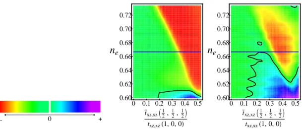
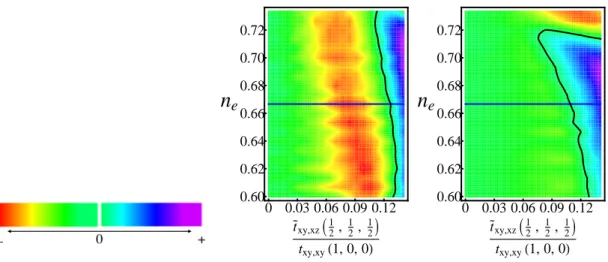
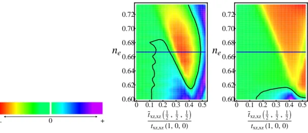
Due to the observed differences in the collective behaviour of the eutectic systems and to the light of the crystallographic composition it is worth to address the fol-lowing issues: i) how does it change the electronic structure close to the Fermi level due to the presence of c-axis stacking faults for both the defect and the host, ii) how the low energy corrections influence the collective behaviour. To handle these questions we study the electronic structure for inhomogeneous systems and we ad-dress the change of the ordered configurations by means of basic criteria for broken symmetry states based on the weak coupling theory of itinerant electron systems. In particular, the analysis aims at underlining the role of the density ne of the Ru bands and the orbital dependent charge transfer between the host and the impurity assuming they are of the n=1 and n=2 type of the RP series. We demonstrate that due to spectral weight redistribution the overall response is inhomogeneous and not always concorde between the impurity and the host. Moreover, due to the multi-orbital character of the ruthenates electronic structure the consequences on the broken symmetry instabilities turns out to be highly orbital dependent too.

The chapter is organized as follows. In the paragraph 2 we introduce the model used to analyse the change in the electronic structure and the consequences on the collective properties. In the paragraph 3 the results related to the modification of the density of states at the Fermi level for the planar inclusion and nearby the defect are presented. The paragraph 4 is devoted to the concluding remarks.

3.2 Model

The eutectic system is modelled by means of an effective tight-binding inhomoge-neous multiband Hamiltonian. The Hamiltonian includes only the orbital degree of freedom close to the Fermi level originated from the t2g bands of the Ru ion and

takes into account the connectivity between the Ru atoms in terms of its first- and second-nearest neighbors within both the single- and the bilayer domains.