Measurements of resonant scattering in the Perseus Cluster core with Hitomi SXS

arXiv:1710.04648v1 [astro-ph.HE] 12 Oct 2017

doi: 10.1093/pasj/xxx000

Measurements of resonant scattering in the

Perseus cluster core with Hitomi SXS

∗

Hitomi Collaboration, Felix A

, Hiroki A

, Fumie

A

, Steven W. A

, Lorella A

, Marc A

,

Hisamitsu A

, Magnus A

, Aya B

, Marshall W.

B

, Roger B

, Laura W. B

, Gregory V.

B

, Esra B

, Edward M. C

, Maria C

,

Meng P. C

, Paolo S. C

, Elisa C

, Jelle

P

,

Cor P.

V

, Jan-Willem

H

, Chris D

, Tadayasu

D

, Ken E

, Megan E. E

, Teruaki E

, Yuichiro

E

, Andrew C. F

, Carlo F

, Adam R. F

,

Ryuichi F

, Yasushi F

, Akihiro F

,

Massimiliano G

, Luigi C. G

, Poshak G

, Margherita

G

, Andrea G

, Liyi G

, Matteo G

, Yoshito

H

, Kouichi H

, Kenji H

, Ilana M. H

,

Isamu H

, Katsuhiro H

, Takayuki H

, Kiyoshi

H

, Junko S. H

, Ann H

, Akio H

,

John P. H

, Yuto I

, Ryo I

, Hajime I

,

Yoshiyuki I

, Manabu I

, Kumi I

, Yoshitaka

I

, Masachika I

, Jelle K

, Tim K

,

Tsuneyoshi K

, Jun K

, Satoru K

, Nobuyuki

K

, Richard L. K

, Caroline A. K

, Takao

K

, Shunji K

, Tetsu K

, Takayoshi

K

, Motohide K

, Katsuji K

, Shu K

,

Peter K

, Hans A. K

, Aya K

, Hideyo

K

, Philippe L

, Shiu-Hang L

, Maurice A.

L

, Olivier O. L

, Michael L

, Knox S.

L

, David L

, Greg M

, Yoshitomo M

, Daniel

M

, Kazuo M

, Maxim M

, Hironori

M

, Kyoko M

, Dan M

C

, Brian R.

M

N

, Missagh M

, Eric D. M

, Jon M. M

,

Shin M

, Kazuhisa M

, Ikuyuki M

, Takuya

M

, Tsunefumi M

, Hideyuki M

, Koji M

, Koji

M

, Hiroshi M

, Richard F. M

, Takao

N

, Hiroshi N

, Takeshi N

, Shinya

N

, Kazuhiro N

, Kumiko K. N

,

Masayoshi N

, Hirofumi N

, Hirokazu O

, Takaya

O

, Masanori O

, Takashi O

, Naomi O

, Masanobu

O

, Frits P

, St ´ephane P

, Robert P

, Ciro

P

, Frederick S. P

, Katja P

, Christopher S.

R

, Samar S

-H

, Shinya S

, Kazuhiro S

, Toru

S

, Goro S

, Kosuke S

, Rie S

, Makoto S

,

Norbert S

, Peter J. S

, Hiromi S

, Megumi

S

, Aurora S

, Randall K. S

, Yang S

,

Łukasz S

, Yasuharu S

, Satoshi S

, Andrew

S

, Hiroyasu T

, Hiromitsu T

, Tadayuki

T

, Shin´ıchiro T

, Yoh T

, Toru T

,

Takayuki T

, Takaaki T

, Yasuo T

, Yasuyuki T.

T

, Makoto S. T

, Yuzuru T

, Yukikatsu T

,

Yuichi T

, Francesco T

, Hiroshi T

, Yohko

T

, Masahiro T

, Hiroshi T

, Takeshi Go T

,

Hiroyuki U

, Hideki U

, Yasunobu U

, Shutaro

U

, Yoshihiro U

, Shin´ıchiro U

, C. Megan U

, Eugenio

U

, Shin W

, Norbert W

, Dan R. W

,

Brian J. W

, Shinya Y

, Hiroya Y

, Kazutaka

Y

, Noriko Y. Y

, Makoto Y

, Shigeo

Y

, Tahir Y

, Yoichi Y

, Daisuke Y

, Irina

Z

, Abderahmen Z

, Maki F

, Anna

O

1_{Dublin Institute for Advanced Studies, 31 Fitzwilliam Place, Dublin 2, Ireland} 2_{Max-Planck-Institut f ¨ur Kernphysik, P.O. Box 103980, 69029 Heidelberg, Germany} 3_{Gran Sasso Science Institute, viale Francesco Crispi, 7 67100 L’Aquila (AQ), Italy}

4_{SRON Netherlands Institute for Space Research, Sorbonnelaan 2, 3584 CA Utrecht, The}

Netherlands

5_{Institute for Space-Earth Environmental Research, Nagoya University, Furo-cho, Chikusa-ku,}

Nagoya, Aichi 464-8601

6_{Kavli Institute for Particle Astrophysics and Cosmology, Stanford University, 452 Lomita Mall,}

Stanford, CA 94305, USA

7_{Department of Physics, Stanford University, 382 Via Pueblo Mall, Stanford, CA 94305, USA} 8_{SLAC National Accelerator Laboratory, 2575 Sand Hill Road, Menlo Park, CA 94025, USA} 9_{NASA, Goddard Space Flight Center, 8800 Greenbelt Road, Greenbelt, MD 20771, USA} 10_{Department of Astronomy, University of Geneva, ch. d’ ´Ecogia 16, CH-1290 Versoix,}

Switzerland

11_{Department of Physics, Ehime University, Bunkyo-cho, Matsuyama, Ehime 790-8577} 12_{Department of Physics and Oskar Klein Center, Stockholm University, 106 91 Stockholm,}

Sweden

13_{Department of Physics, The University of Tokyo, 7-3-1 Hongo, Bunkyo-ku, Tokyo 113-0033} 14_{Research Center for the Early Universe, School of Science, The University of Tokyo, 7-3-1}

Hongo, Bunkyo-ku, Tokyo 113-0033

15_{Kavli Institute for Astrophysics and Space Research, Massachusetts Institute of Technology,}

77 Massachusetts Avenue, Cambridge, MA 02139, USA

16_{Smithsonian Astrophysical Observatory, 60 Garden St., MS-4. Cambridge, MA 02138, USA} 17_{Lawrence Livermore National Laboratory, 7000 East Avenue, Livermore, CA 94550, USA} 18_{Department of Physics and Astronomy, Wayne State University, 666 W. Hancock St, Detroit,}

MI 48201, USA

19_{Department of Astronomy, Yale University, New Haven, CT 06520-8101, USA} 20_{Department of Physics, Yale University, New Haven, CT 06520-8120, USA}

21_{Centre for Extragalactic Astronomy, Department of Physics, University of Durham, South}

Road, Durham, DH1 3LE, UK

22_{Japan Aerospace Exploration Agency, Institute of Space and Astronautical Science, 3-1-1}

Yoshino-dai, Chuo-ku, Sagamihara, Kanagawa 252-5210

23_{Department of Astronomy, Kyoto University, Kitashirakawa-Oiwake-cho, Sakyo-ku, Kyoto}

606-8502

24_{The Hakubi Center for Advanced Research, Kyoto University, Kyoto 606-8302}

25_{Department of Physics, Tokyo Metropolitan University, 1-1 Minami-Osawa, Hachioji, Tokyo}

192-0397

26_{Institute of Astronomy, University of Cambridge, Madingley Road, Cambridge, CB3 0HA, UK} 27_{Faculty of Mathematics and Physics, Kanazawa University, Kakuma-machi, Kanazawa,}

Ishikawa 920-1192

28_{School of Science, Hiroshima University, 1-3-1 Kagamiyama, Higashi-Hiroshima 739-8526} 29_{Fujita Health University, Toyoake, Aichi 470-1192}

30_{Physics Department, University of Miami, 1320 Campo Sano Dr., Coral Gables, FL 33146,}

USA

31_{Department of Astronomy and Physics, Saint Mary’s University, 923 Robie Street, Halifax,}

NS, B3H 3C3, Canada

32_{Department of Physics and Astronomy, University of Southampton, Highfield, Southampton,}

SO17 1BJ, UK

33_{Laboratoire APC, 10 rue Alice Domon et L ´eonie Duquet, 75013 Paris, France} 34_{CEA Saclay, 91191 Gif sur Yvette, France}

35_{European Space Research and Technology Center, Keplerlaan 1 2201 AZ Noordwijk, The}

Netherlands

36_{Department of Physics and Astronomy, Aichi University of Education, 1 Hirosawa,}

Igaya-cho, Kariya, Aichi 448-8543

37_{Department of Physics, Tokyo University of Science, 2641 Yamazaki, Noda, Chiba,}

278-8510

38_{Department of Physics, University of Maryland Baltimore County, 1000 Hilltop Circle,}

Baltimore, MD 21250, USA

39_{Department of Applied Physics and Electronic Engineering, University of Miyazaki, 1-1}

Gakuen Kibanadai-Nishi, Miyazaki, 889-2192

40_{Department of Physics, Nagoya University, Furo-cho, Chikusa-ku, Nagoya, Aichi 464-8602} 41_{Department of Earth and Space Science, Osaka University, 1-1 Machikaneyama-cho,}

Toyonaka, Osaka 560-0043

42_{Department of Physics, Kwansei Gakuin University, 2-1 Gakuen, Sanda, Hyogo 669-1337} 43_{Department of Physics, Rikkyo University, 3-34-1 Nishi-Ikebukuro, Toshima-ku, Tokyo}

171-8501

44_{Department of Physics and Astronomy, Rutgers University, 136 Frelinghuysen Road,}

Piscataway, NJ 08854, USA

45_{Meisei University, 2-1-1 Hodokubo, Hino, Tokyo 191-8506}

46_{Leiden Observatory, Leiden University, PO Box 9513, 2300 RA Leiden, The Netherlands} 47_{Research Institute for Science and Engineering, Waseda University, 3-4-1 Ohkubo,}

Shinjuku, Tokyo 169-8555

48_{Department of Physics, Chuo University, 1-13-27 Kasuga, Bunkyo, Tokyo 112-8551}

49_{Department of Physics, Tokyo Institute of Technology, 2-12-1 Ookayama, Meguro-ku, Tokyo}

152-8550

50_{Department of Physics, Toho University, 2-2-1 Miyama, Funabashi, Chiba 274-8510} 51_{Department of Physics, Kyoto University, Kitashirakawa-Oiwake-Cho, Sakyo, Kyoto}

606-8502

Ca ˜nada, Madrid, Spain

53_{Universities Space Research Association, 7178 Columbia Gateway Drive, Columbia, MD}

21046, USA

54_{National Science Foundation, 4201 Wilson Blvd, Arlington, VA 22230, USA}

55_{Department of Electronic Information Systems, Shibaura Institute of Technology, 307}

Fukasaku, Minuma-ku, Saitama, Saitama 337-8570

56_{Department of Astronomy, University of Maryland, College Park, MD 20742, USA} 57_{Space Telescope Science Institute, 3700 San Martin Drive, Baltimore, MD 21218, USA} 58_{Institute of Physical and Chemical Research, 2-1 Hirosawa, Wako, Saitama 351-0198} 59_{Department of Physics, Tokyo University of Science, 1-3 Kagurazaka, Shinjuku-ku, Tokyo}

162-8601

60_{Department of Physics, University of Wisconsin, Madison, WI 53706, USA}

61_{Department of Physics and Astronomy, University of Waterloo, 200 University Avenue West,}

Waterloo, Ontario, N2L 3G1, Canada

62_{Department of Astronomy, University of Michigan, 1085 South University Avenue, Ann}

Arbor, MI 48109, USA

63_{Okinawa Institute of Science and Technology Graduate University, 1919-1 Tancha,}

Onna-son Okinawa, 904-0495

64_{Hiroshima Astrophysical Science Center, Hiroshima University, Higashi-Hiroshima,}

Hiroshima 739-8526

65_{Faculty of Liberal Arts, Tohoku Gakuin University, 2-1-1 Tenjinzawa, Izumi-ku, Sendai,}

Miyagi 981-3193

66_{Faculty of Science, Yamagata University, 1-4-12 Kojirakawa-machi, Yamagata, Yamagata}

990-8560

67_{Department of Physics, Nara Women’s University, Kitauoyanishi-machi, Nara, Nara}

630-8506

68_{Department of Teacher Training and School Education, Nara University of Education,}

Takabatake-cho, Nara, Nara 630-8528

69_{Frontier Research Institute for Interdisciplinary Sciences, Tohoku University, 6-3}

Aramakiazaaoba, Aoba-ku, Sendai, Miyagi 980-8578

70_{Astronomical Institute, Tohoku University, 6-3 Aramakiazaaoba, Aoba-ku, Sendai, Miyagi}

980-8578

71_{Astrophysics Laboratory, Columbia University, 550 West 120th Street, New York, NY 10027,}

USA

72_{Department of Physics and Astronomy, University of Manitoba, Winnipeg, MB R3T 2N2,}

Canada

73_{Department of Physics and Mathematics, Aoyama Gakuin University, 5-10-1 Fuchinobe,}

Chuo-ku, Sagamihara, Kanagawa 252-5258

74_{Astronomical Observatory of Jagiellonian University, ul. Orla 171, 30-244 Krak ´ow, Poland} 75_{RIKEN Nishina Center, 2-1 Hirosawa, Wako, Saitama 351-0198}

76_{Max-Planck-Institut f ¨ur extraterrestrische Physik, Giessenbachstrasse 1, 85748 Garching ,}

Germany

77_{Department of Physics, Saitama University, 255 Shimo-Okubo, Sakura-ku, Saitama,}

338-8570

78_{Department of Physics, University of Maryland Baltimore County, 1000 Hilltop Circle,}

Baltimore, MD 21250, USA

79_{Department of Physics, University of Rome “Tor Vergata”, Via della Ricerca Scientifica 1,}

I-00133 Rome, Italy

80_{Faculty of Education, Shizuoka University, 836 Ohya, Suruga-ku, Shizuoka 422-8529} 81_{Faculty of Health Sciences, Nihon Fukushi University , 26-2 Higashi Haemi-cho, Handa,}

82_{MTA-E ¨otv ¨os University Lend ¨ulet Hot Universe Research Group, P ´azm ´any P ´eter s ´et ´any 1/A,}

Budapest, 1117, Hungary

83_{Department of Theoretical Physics and Astrophysics, Faculty of Science, Masaryk}

University, Kotl ´aˇrsk ´a 2, Brno, 611 37, Czech Republic

∗_{E-mail: ksato@rs.tus.ac.jp, ksksato@phy.saitama-u.ac.jp, zhur@stanford.edu, frits.paerels@gmail.com}

Received ; Accepted

Abstract

Thanks to its high spectral resolution (∼ 5 eV at 6 keV), the Soft X-ray Spectrometer (SXS) on board Hitomi enables us to measure the detailed structure of spatially resolved emission lines from highly ionized ions in galaxy clusters for the first time. In this series of papers, using the SXS we have measured the velocities of gas motions, metallicities and the multi-temperature structure of the gas in the core of the Perseus cluster. Here, we show that when inferring physical properties from line emissivities in systems like Perseus, the resonant scattering effect should be taken into account. In the Hitomi waveband, resonant scattering mostly affects the FeXXVHeα line (w) - the strongest line in the spectrum. The flux measured by Hitomi in this line is suppressed by a factor ∼1.3 in the inner ∼30 kpc, compared to predictions for an optically thin plasma; the suppression decreases with the distance from the center. The w line also appears slightly broader than other lines from the same ion. The observed distortions of the wline flux, shape and distance dependence are all consistent with the expected effect of the resonant scattering in the Perseus core. By measuring the ratio of fluxes in optically thick (w) and thin (FeXXVforbidden, Heβ, Lyα) lines, and comparing these ratios with predictions from Monte Carlo radiative transfer simulations, the velocities of gas motions have been obtained. The results are consistent with the direct measurements of gas velocities from line broadening described elsewhere in this series, although the systematic and statistical uncertainties remain significant. Further improvements in the predictions of line emissivities in plasma models, and deeper observations with future X-ray missions offering similar or better capabilities to the Hitomi SXS will enable resonant scattering measurements to provide powerful constraints on the amplitude and anisotropy of clusters gas motions.

Key words: galaxies: clusters: individual (the Perseus cluster) – X-rays: galaxies: clusters – galaxies: clusters: intracluster medium

1 Introduction

− 108 K) gas in the intra-cluster medium (ICM) is optically thin to the continuum X-ray radiation, meaning that galaxy clusters are transparent to their own X-ray contin-uum photons. However, Gilfanov et al. (1987) showed that the strongest X-ray resonance lines can have significant opti-cal depths, of order unity or larger. Line photons can therefore undergo resonant scattering (hereafter RS), that is, they can be absorbed by ions and be almost instantaneously re-emitted in a different direction. As a result of this scattering, the emission line intensity is reduced in the direction of the center of the clus-ter (generally the region of largest optical depth along our line of sight), and enhanced towards the outskirts (e.g. see review

∗_{The corresponding authors are Kosuke SATO, Irina ZHURAVLEVA, Frits}

PAERELS, Maki FURUKAWA, Masanori OHNO, Megan ECKART, Akihiro FURUZAWA, Caroline KILBOURNE, and Maurice LEUTENEGGER

by Churazov et al. 2010). Even if the RS effect is not strong, it will affect the spatially resolved measurement of elemental abundances in the ICM (e.g. B¨ohringer et al. 2001; Sanders et al. 2004), distort the profiles of X-ray surface brightness (e.g. Gilfanov et al. 1987; Shigeyama 1998), and can lead to up to tens of percent polarization of the line radiation (Sazonov et al. 2002; Zhuravleva et al. 2010).

There have been numerous attempts to detect the RS effect in X-ray spectra of the Perseus Cluster (e.g. Molendi et al. 1998; Ezawa et al. 2001; Churazov et al. 2004) and other clusters (e.g. Kaastra et al. 1999; Akimoto et al. 2000; Mathews et al. 2001; Sakelliou et al. 2002; Sanders & Fabian 2006). However, the results remain somewhat controversial. More recently it was shown for the Perseus Cluster that the energy resolutions of the CCD-type spectrometers on XMM-Newton and Chandra are not sufficient to uniquely and robustly distinguish between

spectral distortions due to RS, different metal abundance pro-files, and/or levels of gas turbulence (Zhuravleva et al. 2013).

Here we present Hitomi observations of the RS effect in the core of the Perseus Cluster. Due to the superb energy resolution (FWHM ∼ 5 eV at 6 keV) of the non-dispersive Soft X-ray Spectrometer (SXS) on-board Hitomi, individual spectral lines are resolved (Hitomi Collaboration et al. 2016), allowing us to measure the suppression of the flux in the He-like Fen = 1 − 2 resonance line at 6.7 keV for the first time. As we discuss below, this suppression is likely due to photons having been scattered out of the line of sight.

Given that the optical depth at the center of a line depends on the turbulent Doppler broadening, the comparison of fluxes for optically thin and thick lines can be used to measure the characteristic amplitude of gas velocities in the ICM, comple-menting direct velocity measurements via Doppler broadening and centroid shifts. The RS technique has previously been successfully applied to high-resolution spectra from the cool (kT ∼ 1 keV), dense cores of massive elliptical galaxies and galaxy groups, using deep XMM-Newton observations with the Reflection Grating Spectrometer (RGS). Detailed study of those data showed that the FeXVIIresonance line at 15.01 ˚A is sup-pressed in the dense galaxy cores, but not in the surrounding regions, while the line at 17.05 ˚A from the same ion is opti-cally thin and is not suppressed (e.g. Xu et al. 2002; Kahn et al. 2003; Hayashi et al. 2009; Pinto et al. 2016; Ahoranta et al. 2016). Performing modeling of the RS effect, accounting for different levels of turbulence, revealed random gas velocities of order ∼ 100 km s−1_{in many elliptical galaxies and groups (e.g.}

Werner et al. 2009; de Plaa et al. 2012; Ogorzalek et al. 2017). Doppler spectroscopy and the RS technique provide com-plementary, non-redundant constraints on the velocity field. A measurement of the Doppler broadening along a given line of sight depends on the line-of-sight integral of the velocity field weighted by the square of the density. In contrast, the RS effect probes the integral of the velocity field along photon trajecto-ries, weighted by the density itself. Even more striking, if tur-bulence is isotropic, the measurements of the Doppler effect and RS should provide the same results. If the measured velocities differ, this may indicate that the velocity field is anisotropic. Namely, if motions are radial (tangential) the scattering effi-ciency is reduced (increased) compared to the isotropic case (Zhuravleva et al. 2011). It is also important to note that the RS technique is mostly sensitive to small-scale motions (Zhuravleva et al. 2011). The comparison between the two mea-surements of the velocity field can also reveal large scale devi-ations from spherical symmetry, and density inhomogeneities.

Hitomi Collaboration et al. (2016) mentioned the presence of the RS effect in the Perseus core. The measured ratio of the FeXXVHeα resonance to forbidden line fluxes, 2.48±0.16 with 90% statistical uncertainties, is smaller than the predicted ratio

in optically thin plasma with mean gas temperature of 3.8 keV. Hitomi Collaboration et al. (2016) also reports velocity disper-sions of187 ± 13 and 164 ± 10 km s−1_{in the core and outer}

regions, respectively. Theoretical studies of the RS effect pre-dict that the resonance line flux should be still suppressed if gas is moving with such velocities in the Perseus Cluster. In this paper, we measure spatial variations of line ratios and widths using the improved calibration data and taking systematic un-certainties into account. We confirm the presence of the RS effect and, using numerical simulations of radiative transfer in the Perseus Cluster, infer the velocities of gas motions. We refer the reader to Hitomi collaboration et al. (2017e, 2017d, 2017b, 2017c) papers for the most complete analysis of spectroscopic velocity measurements, details of the plasma modeling and de-tailed measurements of the temperature structure1_{. The ICM} parameters present in this paper are consistent with the mea-surements in these papers; small variations of specific parame-ters do not affect our conclusions.

The structure of our paper is as follows. In section 2, we describe the observations and data reduction. In section 3, we demonstrate that the complex coupled spectral and spatial be-havior of the emission line intensities in the FeXXVHeα spec-trum are qualitatively consistent with the presence of RS. In section 4, we measure line intensity ratios that are sensitive to RS, as a function of position in the cluster. In section 5, we describe the radiative transfer simulations performed. We used two independent simulation codes: one based on the software packages of Geant4 tool kit2and HEAsim3, and one custom-written by one of us (IZ) based on Sazonov et al. (2002); we will refer to this latter code as the ICM Monte Carlo code or ’ICMMC code’. In section 6, we compare the results of simu-lations with the measured line ratios, and derive constraints on the turbulent velocity field. In section 7, we discuss the uncer-tainties associated with the atomic excitation rates, and possible presence of additional excitation processes such as charge ex-change. The results are summarized and discussed in section 8.

Throughout this paper we adopt AtomDB version 3.0.84_, and the plasma emission models in APEC5. All data analy-sis software tasks refer to the HEAsoft package6_{. We adopt a} Galactic hydrogen column density ofNH= 1.38 × 1021cm−2

(Kalberla et al. 2005) in the direction of the Perseus Cluster, and use the solar abundance table provided by Lodders & Palme (2009). Unless noted otherwise, the errors are the 68% (1σ) confidence limits for a single parameter of interest.

1_{We will refer these papers as the “Atomic” or “A”, the “Velocity” or “V”, the}

“Temperature” or “T”, and the “Abundance” or “Z” papers, respectively.

2_{http://geant4.cern.ch} 3

https://heasarc.gsfc.nasa.gov/ftools/caldb/help/heasim.html

4_{http://www.atomdb.org}

5_{Astrophysical Plasma Emission Code; http://www.atomdb.org} 6_{https://heasarc.nasa.gov/lheasoft}

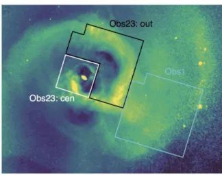
Fig. 1. The Hitomi SXS observation regions overlaid on the Chandra

X-ray image of the Perseus Cluster in the 1.8–9.0 keV band divided by the spherically-symmetric model for the surface brightness. In this paper we will consider obs23 cen as the central region, which includes the central AGN (white), outer region obs23 out (black) and obs1 whole (cyan).

2 Observation & data reduction

Hitomi carried out a series of 4 overlapping pointed obser-vations of the Perseus Cluster core during its commissioning phase in 2016 February and March, with a total of 340 ks ex-posure time (Table 1). The Hitomi SXS is a system that com-bines an ray micro-calorimeter spectrometer with a Soft X-ray Telescope (SXT) to cover a 3 × 3 arcmin field of view (FOV) with an angular resolution of 1.2 arcmin (half power di-ameter). The micro-calorimeter spectrometer provided a spec-tral energy resolution of ∆E ∼ 5 eV at 6 keV (Kelley et al. 2016). It is operated inside a dewar, in which a multi-stage cooling system maintains a stable environment at 50 mK; tem-perature stability is important to give such a high energy res-olution. The SXS was originally expected to cover the energy range between 0.3 and 12 keV, but only data in the E >∼ 2 keV band were available during the Perseus observations be-cause the gate valve on the SXS dewar, which consists of a Be window and its support structure, was still closed at the time of observation. The other instruments on Hitomi are described in Takahashi et al. (2017). In this paper, we use only the SXS data for investigating RS in the Perseus cluster core.

The Perseus Cluster was observed four times with Hitomi over a ten day period, but the SXS dewar had not yet achieved thermal equilibrium during the first two observations. A drift in temperature of the detector implies a drift in the photon energy to signal conversion (the so-called ’gain’). For the observations during which the gain drift was significant, the photon energy scale was determined using data processing routine sxsperseus in HEAsoft, which corrects the gain scale via an extrapolation of the relationship between the relative gain changes on the ar-ray and on the continuously illuminated calibration pixel from

the Perseus observation to the later full-array calibration in the official data pipeline processing. Observations 1 and 2 in table 1 were affected by this gain drift; observations 3 and 4 were obtained under thermal equilibrium in the SXS dewar. A dif-ference in gain between obs. 2, and the sum of obs. 3 and 4 (full FOV) of ∼ 2 eV can still be seen (Eckart et al. 2017). It is most clearly seen around the FeXXVHeα line complex in the official data pipeline processing (Angelini et al. 2016). Not surprisingly, obs. 1 has a much larger energy scale uncertainty (Porter et al. 2016). All pixels in the micro-calorimeter array are independent, and in principle each has its own energy scale, and energy scale variations.

In our spectral analysis of the central region in section 4 we have to take the contribution of non-thermal emission from the central AGN in the Perseus Cluster, NGC 1275, explicitly into account. Following the T paper, we applied the “sxsextend” task to register event energies above 16 keV, so that we can construct the spectrum up to ∼20 keV. This is crucial to dis-criminate the AGN and cluster gas components spectrally, as the former dominates the spectrum in the extended energy band. This method is same as that in the “T” paper (Hitomi collabo-ration et al. 2017b). After having added the high energy events, and having applied the extra screenings, we adopted two extra gain corrections, similar to the procedures described in the “A” paper (Hitomi collaboration et al. 2017e), but used the differ-ent reference redshift of 0.017284 according to the “V” paper (Hitomi collaboration et al. 2017d). The detailed correction pa-rameters were shown in the appendix in the “T” paper (Hitomi collaboration et al. 2017b). The first of these corrections is re-ferred to as the “z-correction”, which adjusts the absolute en-ergy scale of each pixel in each data set such that the redshift of the FeXXVHeα resonance line is aligned to the redshift of NGC 1275 atz = 0.017284. The second is referred to as the “quadratic-curve-correction”, which applies a second-order cor-rection, centered on FeXXVHeα, to take out a small apparent offsets in the observed energies of the strongest emission lines across the 1.8–9 keV band. The intent of the “z-correction” is to allow the spectra from different pixels and different pointings to be added with minimal broadening of the lines from variation in the bulk velocity across the Perseus cluster within the SXS FOV. For the RS analysis we need to measure the ratios of line fluxes, thus we use the full available data set to reduce statistical un-certainties on measured line ratios, presuming variations across the data set are sufficiently small to warrant this approach. The uncertainties in the RS analysis associated with the energy scale corrections are discussed in section 4.

After applying all these corrections, the spectra were ex-tracted with the Xselect package in HEAsoft for each region as shown in figure 2. We used only high primary grade event data to generate the spectra. In order to subtract the non-X-ray background (NXB), we employed the day and dark Earth

Table 1. Hitomi Observations of the Perseus Cluster

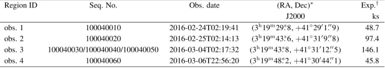
Region ID Seq. No. Obs. date (RA, Dec)∗ _Exp.†

J2000 ks obs. 1 100040010 2016-02-24T02:19:41 (3h₁₉m_29.s_8,+41◦₂₉′_1.′′_{9) 48.7} obs. 2 100040020 2016-02-25T02:14:13 (3h₁₉m_43.s_6,+41◦₃₁′_9.′′_{8) 97.4} obs. 3 100040030/100040040/100040050 2016-03-04T02:17:32 (3h19m43.s 8,+41◦₃₁′_12.′′_{5) 146.1} obs. 4 100040060 2016-03-06T22:56:20 (3h₁₉m_48.s_2,+41◦₃₀′_44.′′_{1) 45.8} ∗_{Average pointing direction of the Hitomi SXS, as recorded in the RA NOM and DEC NOM keywords of the event FITS files.} †_{After screening on rise time cut and for events that occur near in time to other events}

database using the “sxsnxbgen” Ftools task. We generated a redistribution matrix file (RMF) including the escape peak and electron loss continuum effects with the “whichrmf=x” option in the “sxsmkrmf” task to represent the spectral shape in the lower and higher energy band. Because the spatial distributions of the ICM and AGN components are different, we also made two kinds of Ancillary Response Files (ARFs) for the spectrum of each region,AP _andAC_{. The responseA}P _assumed

point-like source emission from NGC 1275 centered on (RA, Dec.) = (3h₁₉m_48.s_1,+41◦₃₀′₄₂′′_{); whileA}C_{is appropriate to the}

dif-fuse emission from the ICM, and is based on the X-ray image observed with Chandra in the 1.8–9.0 keV energy band, with a region of radius 10 arcseconds centered on the AGN replaced with the average surrounding brightness by the “aharfgen” task in HEAsoft. At the time operations ceased, a full in-orbit cal-ibration of the spatial response and effective area had not yet been performed well. In this paper, we therefore use ARFs gen-erated based on the ground calibration of SXT. A ’fudge factor’ was derived from the ground measurements, to adjust the cali-bration to in-flight performance; however this fudge factor has large uncertainties as shown in Tsujimoto et al. (2017); Hitomi collaboration et al. (2017b), and the spectral fits with these “fudged” ARFs produced artificial residual features. We also examined an adjustment of “Crab ratio” using the Crab obser-vation with Hitomi SXS (Tsujimoto et al. 2017), however this adjustment also introduced systematic residuals around the Au and Hg edges around 12 keV as shown in the “T” paper (Hitomi collaboration et al. 2017b). We therefore decided not to apply such corrections and use the standard ground calibration-based response. Finally, in all spectral fits, the spectra are grouped with 1 eV bin−1_{, and 1 count per bin at least, allowing the}

C-statistics method to be used.

We extracted spectra from three regions, obs23 cen and obs23 out from obs. 2 and 3, and obs1 whole from obs. 1, with the region boundaries coinciding with detector pixel boundaries as shown in figure 1, in order to avoid having to redistribute pho-tons between pixels. The pointing directions of obs. 2 and 3 are slightly different (offset by ∼ 0.1 arcmin), however, this offset is much smaller than the size of the SXS point spread function. The obs23 cen, obs23 out, and obs1 whole are located on the

central 9 pixels around the AGN, the outer 26 pixels of obs. 2 and 3, and the whole region of obs. 1, respectively, see figure 1. The observed spectra in the 6.1–7.9 keV band are shown in figure 2. Their modeling is discussed below in section 4.

3 Observational indications for resonant

scattering

Theoretical studies of the RS effect in the Perseus Cluster pre-dict that, in the absence of gas motions the degree of flux sup-pression in the resonance line of He-like Fe should vary with the projected distance from the cluster center: the line flux will be most suppressed in the innermost region, with the suppres-sion decreasing with projected distance out to a radius ∼ 100 kpc. At larger radii, the line flux is slightly increased relative to the value for the optically thin case (e.g. Churazov et al. 2004). Also, as the result of scattering, the wings of the line become slightly stronger (see e.g. Zhuravleva et al. 2013). Below we demonstrate that the Perseus Hitomi data show evidence for both of these effects.

3.1 Flux suppression in the FeXXVHeα resonance line

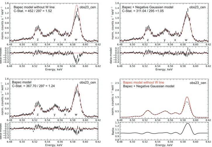
We first consider the spectrum of the He-like FeXXV triplet from the innermost region (obs23 cen in figure 1), where the suppression of the resonance (w) line is expected to be the strongest. A single-temperature bapec7_{model for an optically} thin plasma can approximately model the resonance line flux, but will then underestimate the fluxes of the neighboring forbid-den (z) and intercombination (y) lines (see bottom left panel in figure 3 and supplementary material in Hitomi Collaboration et al. (2016)). Exclusion of the resonance line from the modeling provides a better fit forx, y and z and other weaker lines, but clearly overestimates thew flux (top left panel in figure 3). We then add a Gaussian component to the model with the energy of thew line and normalization that is allowed to be negative. The best-fitting result of this model is shown in the top right

7_{The bapec model describes a plasma in collisional ionization equilibrium,}

with arbitrary velocity broadening in addition to thermal Doppler broaden-ing, and element abundance ratios relative to He fixed to the Solar ratios.

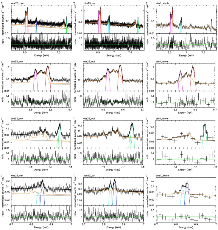
Fig. 2. The observed Hitomi spectra extracted from the obs23 cen, obs23 out and obs1 whole regions shown in figure 1, and binned for display purposes.

Top panels show the resultant spectral fits in 6.1–7.9 keV band, while the second, third and fourth rows show the energy range of the Heα complex, and Heβ, and Lyα lines in 6.4–6.7, 7.5–7.8, and 6.7–7 keV, respectively. The spectra obtained with the Hitomi SXS are shown in black; light gray lines show the emission from the AGN. Orange lines indicate the “modified” bvvapec model, in which the strongest lines have been deleted. The FeXXVHeα forbidden and resonance, Heβ1,2, and FeXXVILyα1,2are shown in magenta, red, green, light green, blue and cyan lines, respectively. The lower panels show the fit residuals in units

of ratio.

panel in figure 3. The best-fitting normalization of the Gaussian component is indeed negative and the model provides a

statisti-cally better fit to the data than a pure bapec model8_{. The ratio} of the best-fitting models shown in the top panels shows a

sup-8_{For all three modeling steps we use the same gas temperature, which is}

Bapec model without W line C-Stat. = 452 / 297 = 1.52 obs23_cen w z y x obs23_cen Bapec + Negative Gaussian model

C-Stat. = 311.04 / 295 =1.05 obs23_cen Bapec model C-Stat. = 367.70 / 297 = 1.24 w z y x w z y x

Bapec model without W line

Bapec + Negative Gaussian model

obs23_cen

Fig. 3. Flux suppression in the strongest line of He-like FeXXV(w) in the Perseus Cluster observed in the obs23 cen region. Black points show the Hitomi

data; red lines in the corresponding panels show the best-fitting models. Top left: the spectrum is fitted with the bapec model, excluding thew line from the data; top right: the same spectrum is fitted with the bapec model and a Gaussian component centered at the energy of thew line, the normalization of the Gaussian model is allowed to be negative; bottom left: the same spectrum fitted with the bapec model. The comparison of the models from the top left (solid) and right (dashed) panels is shown in the bottom right panel. The suppression of thew line indicates the presence of the resonant scattering effect in the Perseus Cluster. See Section 3.1 for details.

Bapec model without W line

Bapec + Negative Gaussian model

obs23_out _{Bapec model without W line} obs1_whole

Bapec + Negative Gaussian model

Fig. 4. The same as the bottom right panel in figure 3, but for the spectra observed in obs23 out (left) and obs1 whole (right) regions. See Section 3.1 for

pression of the resonance line by a factor of ∼ 1.28, indicating the presence of RS.

The same modeling procedure is applied to spectra from the regions at larger distances from the cluster center (obs23 out and obs1 whole, see figure 1). When fitting the obs23 out spec-trum, the bapec+negative Gaussian model provides a statisti-cally better fit than the pure bapec model. Thew flux in the obs23 out region is suppressed by factor of ∼ 1.28 (left panel in figure 4). In the most distant from the cluster center region, obs1 whole, the bapec+negative Gaussian model does not pro-vide a statistically better fit of the data than a bapec model. The measured line suppression is small, less than 1.15 (right panel in figure 4). These simple experiments illustrate the possible presence of the RS effect in the Perseus core.

3.2 The broadening of the FeXXVHeα resonance line

In addition to flux suppression in the resonance line, the RS broadens the wings of the line. Even though the effect is signif-icantly smaller than the line suppression, we have checked for indications of line broadening in thew line compared to other lines in the triplet. We fit the observed data excluding thew line with a single-temperature bapec model, from which thew line has been removed. Freezing the best-fitting parameters of this model, we fit the whole triplet, with thew line restored, adding an additional Gaussian component with the central energy of thew line. Such modeling allows us to measure the broadening of thew line independently from the broadening of other lines in the triplet. Accounting for statistical uncertainties, the turbu-lent broadening of thew line varies between 171–183 km s−1_,

while the broadening of thex, y and z lines are smaller, 145– 165 km s−1_{. A similar difference is observed in the obs23 out}

region. Namely, thew line turbulent broadening in this region is 159–167 km s−1_{, while in all other lines it is 136–150 km}

s−1_.

4 Observed line ratios

We fitted the spectra with a combination of emission mod-els representing the AGN and the ICM, each with its own response, in Xspec. The AGN is represented by a power-law with redshifted absorption, with additional (redshifted) Fe Kα1, 2 fluorescent emission lines; the ICM is modeled

with a redshifted collisional ionization equilibrium plasma, with adjustable elemental abundances, and additional Gaussian emission lines if necessary. The two components share a common foreground neutral Galactic absorption. Formally, we have AGN model: T BabsGAL × (pegpwrlwAGN+

zgaussAGN, FeKα1+ zgaussAGN, Fe Kα2), and ICM model:

T BabsGAL× (bvvapecICM+ zgaussFe lines). The AGN

pa-rameters are fixed at the numbers in the NGC 1275 paper (Hitomi collaboration et al. 2017a). In this paper, we modify the bvvapecmodel, setting the emissivities of the strong Fe lines to zero.

Firstly, we derived the ICM temperature, Fe abundance, tur-bulent velocity, and normalizations from the spectral fits in 1.8– 20.0 keV with a single temperature model for each region. In the broad band fit, to determine those parameters, we adopted the modified bvvapec model, from which the FeXXVHeα reso-nance line is excluded, and the corresponding Gaussian model is added. The resultant parameters and C-statistics from the spec-tral fits for each region are shown in table 2. The “projected” temperature increases slightly with radius, while the Fe abun-dance drops by ∼ 0.1 solar from the center to the obs1 whole region. The measured temperature and Fe abundance gradients agree with the results from the “T” and “Z” papers (Hitomi col-laboration et al. 2017b, 2017c). As for the turbulent velocity, σv, the derived values are almost constant with radius. These

σv in the previous Hitomi paper (Hitomi Collaboration et al.

2016) and “V” paper (Hitomi collaboration et al. 2017d) are slightly different. We note that the data reduction, calibrations and plasma codes are more improved than the previous Hitomi paper. And, the numbers shown in table 4 for PSF uncorrected in the “V” paper from their narrow band fits in 6.4–6.7 keV are slightly smaller than those from the broadband fits shown in ta-ble 2 in this paper. The difference comes from the broader line width of the Lyα lines (see table 2 and the “V” paper).

Fixing the ICM temperature, Fe abundance, andσv at the

values from the broad band fits, we exclude the FeXXVHeα forbidden (z) and resonance (w), the Heβ and the FeXXVILyα lines from the bvvapec model and include Gaussian line models instead with the central energies of these lines. The best-fitting normalizations of the Gaussian components give total fluxes of these lines. Here, the line widths of the Lyα2 and Heβ2 are

linked to Lyα1 and Heβ1lines, respectively, and other

param-eters except for the redshift are varied in the spectral fits. This fitting model is very useful since bvvapec describes the weak satellite lines, while the added Gaussian lines allow us to mea-sure the fluxes of the strongest emission lines in a model inde-pendent way, taking blending with weaker emission lines into account.

The observed spectra are well-described by the model, ex-cept around the 6.55 keV feature, as shown in figure 2. The resulting line ratios and widths (thermal and turbulent broaden-ings,σv+th) are summarized in table 2 and figure 5. The Lyα1

and Lyα2lines are clearly resolved in obs23 cen and obs23 out

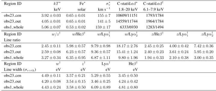
regions, while the Heβ lines are not, due to their close central energies. Note that the emission lines are represented well by the corresponding Gaussian models, as confirmed by the study of possible non-Gaussianity in the “V” paper. The derived ra-dial profile of thew/z ratio increases with the distance from the

Table 2. Summary of the best-fit properties of temperatures, Fe abundance, turbulent velocity (σv), C-statistics, line ratios, and line

widths (σv+th).

Region ID kT∗ _Fe∗ _σ∗

v C-stat/d.o.f∗ C-stat/d.o.f†

keV solar km s−1 _{1.8–20 keV 6.1–7.9 keV}

obs23 cen 3.92 ± 0.03 0.65 ± 0.01 155 ± 7 10609/11151 1793/1784 obs23 out 4.05 ± 0.01 0.65 ± 0.01 141 ± 5 14559/11744 1964/1784 obs1 whole 5.06 ± 0.07 0.53 ± 0.02 159 ± 17 6333/6930 1283/1494

Region ID w/z† _w/Heβ† _w/Lyα†

1 w/Lyα † 2 z/Heβ † _z/Lyα† 1 z/Lyα † 2 Line ratio obs23 cen 2.45 ± 0.11 5.98 ± 0.57 9.79 ± 0.98 18.17 ± 2.76 2.45 ± 0.25 4.00 ± 0.42 7.42 ± 0.36 obs23 out 2.59 ± 0.08 6.23 ± 0.57 9.36 ± 0.57 15.41 ± 1.24 2.40 ± 0.23 3.61 ± 0.24 5.95 ± 0.20 obs1 whole 3.27 ± 0.34 6.35 ± 0.95 6.87 ± 1.11 9.80 ± 1.96 1.94 ± 0.33 2.10 ± 0.38 3.00 ± 0.35

Region ID w† _z† _Lyα† _Heβ†

Line width (σv+th) eV eV eV eV

obs23 cen 4.49 ± 0.11 3.57 ± 0.21 5.29 ± 0.55 3.45 ± 0.50 obs23 out 4.20 ± 0.08 3.54 ± 0.15 3.46 ± 0.25 4.24 ± 0.42 obs1 whole 4.43 ± 0.24 3.58 ± 0.50 6.09 ± 0.89 4.81 ± 0.80

∗_{Fits in the broad 1.8–20.0 keV band with the AGN and modified bvvapec models, from which the resonance line is excluded and a}

Gaussian component is added instead. σvis a turbulent velocity in bvvapec model without the resonance line. The numbers in this table

are slightly smaller than those in the “V” paper (Hitomi collaboration et al. 2017d), see section 4 for the details.

†_{Fits in the narrow, 6.1–7.9 keV, band with the AGN and modified bvvapec models, from which we exclude the He-α resonance and}

forbidden, He-β1&2, and Ly-α1&2 lines.

center, while thez/Heβ ratio is almost the same everywhere. The measuredw line widths in the obs23 cen and obs23 out regions are broader than thez ones at the ∼ 2 σ level. The com-parison of the measured line ratios and line broadening with the results of numerical simulations of the RS effect is discussed in section 5.

Systematic uncertainties, such as (a) the ICM modeling of a single or two temperature structure, (b) gain correction, (c) the point spread function (PSF) deblending, and (d) plasma codes (AtomDB version 3.0.8 or 3.0.9) should be considered in the spectral analysis. Estimates of their effects are examined below. As a result, these uncertainties almost do not affect our results and conclusions.

As for the ICM modeling, the Fe lines in 6–8 keV are well modeled with a single temperature model with the exception of the resonance (w) line shown in figure 2 and table 2. On the other hand, as described in the “T” paper, a two temperature (2T) model improves the spectral fits when AtomDB version is 3.0.9. Thew/z ratios measured from the 1T and 2T models agree within the statistical error with either AtomDB version 3.0.8 or 3.0.9. In this paper, since we examined the spectral fits for the observations and simulations in the same manner, i.e., the same model formula, as described in section 5.3 and com-pare the resultant fit parameters for each other, the choice of the 1T or 2T models does not affect our conclusions, as long as the continuum spectra are well-represented by the models. Note that the gas temperature measured from the line ratios

ob-tained from the 2T model in the “T” paper agree well with the deprojected temperature profile from the Chandra data.

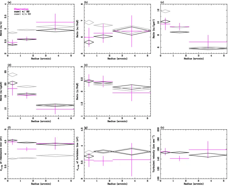
We repeated the spectral analysis using gain-uncorrected Hitomi data to estimate the uncertainty. Figure 6 shows compar-ison plots of the resultant fits for thew/z and z/Heβ line ratios and line widths,σv+th, of thew and z lines between the gain

corrected and uncorrected data. The line ratios from both data sets are consistent within the statistical errors. At the same time, the width of thew line in obs23 cen decreases, as expected, by about 5% when the gain correction is applied. We did not cor-rect the spectral fit for the PSF effects. The azimuth-averaged values in regions 1–4 for the PSF uncorrected numbers in the “V” paper which roughly correspond to the obs23 out region are almost consistent with our results within statistical errors. The PSF effect is accounted for in the simulations in this pa-per described in section 5. The residuals around 6.55 keV in the obs23 out region are likely associated with uncertainties in the plasma model for the FeXXIVLi-like line (see also figure 8 in “Atomic” paper). These come from the underestimation of the Li-like lines in AtomDB version 3.0.8. The updated version 3.0.9 are corrected for the problem as shown in Appendix 1. This feature has negligible impact on our results for line ratios and widths, however, since the Li-like lines are separated from thew and z lines.

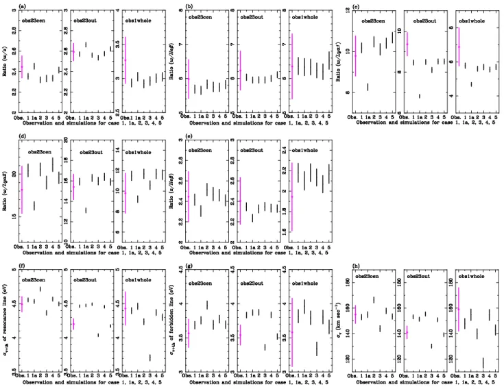
Fig. 5. (a)–(e): Comparisons of the observed and predicted ratios of the Fe Heα resonance (w), Heα forbidden (z), Heβ, and Lyα1,2lines. Observations

are shown as magenta crosses and the simulations with RS as black diamonds and the same without RS as gray diamonds for the assumption of the constant σvof 150 km s−1(case 1). (f)–(g): Comparisons of the widths of the resonance (w) and forbidden (z) lines between observation (magenta crosses) and

simulations with RS (black diamonds) and without RS (gray diamonds). (h): Comparisons of the derived turbulent velocities from the spectral fits between observation (magenta cross) in broad band fits and the simulations.

5 Radiative transfer simulations

The line suppression due to the RS effect is sensitive to the ve-locity of gas motions: the larger the veve-locity of gas motions the lower the probability of scattering and the closer the line ratios to those for an optically thin plasma. In order to interpret the observed line suppression and infer the velocity of gas motions, we performed radiative transfer Monte Carlo (MC) simulations of the RS in the Perseus Cluster. We followed two independent approaches: (i) using the Geant4 and HEAsim tools and as-suming a velocity field consistent with the direct velocity mea-surements as presented in the “V” paper (Hitomi collaboration et al. 2017d), and (ii) using a proprietary code written specifi-cally for MC simulations of radiative transfer in the cluster ICM (ICMMC). Both approaches are based on the emission models

for an optically thin plasma taken from AtomDB version 3.0.8, and take into account projection effects (gas density, temper-ature, abundance of heavy elements) and the spatial response of the telescope. The latter is treated differently in both ap-proaches. The results based on both simulations broadly agree. Details of the two approaches are discussed below.

5.1 Model of the Perseus Cluster

For the MC simulations, we adopt a spherically symmetric model of the Perseus Cluster. We used archival Chandra data to measure the profiles of gas density, temperature and abun-dance of heavy elements. Excluding point sources and the tral AGN, projected spectra are obtained in radial annuli, cen-tered on the central galaxy, NGC 1275. These are deprojected

Fig. 6. Scattering plots between the gain corrected and uncorrected data for (a) the w/z line ratio, (b) the z/Heβ line ratio, (c) w line width (σv+th) and (d) z

line width (σv+th). Open circles, squares, and triangles correspond to the measurements in the obs23 cen, obs23 out, and obs1 whole regions, respectively.

Fig. 7. Model of the Perseus Cluster used for the Monte Carlo simulations of

radiative transfer in strong emission lines. Top: deprojected electron number density; middle: deprojected gas electron temperature; bottom: deprojected abundance of heavy elements relative to Solar abundance from Lodders & Palme (2009). Chandra data are used in the inner ∼ 150 kpc region. These profiles of the temperature and electron density are merged with Suzaku deprojected data at large radii,r >∼ 150 kpc, taken from Urban et al. (2014), and the abundance is adopted to be the averaged number in Werner et al. (2013); Matsushita et al. (2013); Urban et al. (2014).

following the procedure described by Churazov et al. (2003). The spectra are fitted with an apec model in a broad energy band, 0.5–8.5 keV, accounting for Galactic foreground absorp-tion by a column density ofNH= 1.38 × 1021cm−2, and

treat-ing the abundance of heavy elements as a free parameter, ustreat-ing the solar abundance table by Lodders & Palme (2009). The Chandra deprojected profile within ∼ 150 kpc is shown in fig-ure 7. There is a density drop in the innermost region (the first point from the center) likely associated with the bubbles of rel-ativistic plasma that push up the X-ray gas. Due to this density drop and the presence of multi-temperature plasma, the depro-jected temperature and the heavy element abundances are not determined reliably in this region. Therefore, we assume con-stant temperature and abundance profiles in the inner ∼ 10 kpc region. The Chandra deprojected profile is then merged with the Suzaku deprojected data (Urban et al. 2014) at large radii,

r > 150 kpc. As for the abundances in r = 150–1000 kpc, since the observed abundances (∼0.3 solar) from Suzaku in Urban et al. (2014); Werner et al. (2013) are relatively smaller than those (∼0.5 solar) from XMM in Matsushita et al. (2013), we adopted the averaged number of ∼0.4 solar as the input param-eter. Figure 7 shows the combined radial profiles.

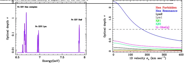
5.2 Optical depth

Using the equations shown in Zhuravleva et al. (2013), the op-tical depth is calculated from the center of the cluster out to a radius corresponding to an angular size on the sky of40′

∼ 830 kpc, corresponding to 2/3 timesr500(Urban et al. 2014). The

left panel of figure 8 shows the optical depth for each line (see also table 3) for the case of zeroσvcalculated using the cluster

model described in section 5.1. RS is expected to be important in the central regions of the Perseus Cluster, where the optical depth is larger than 1. The FeXXVHeα w has the largest optical depth ∼ 2.3, while the FeXXVHeα z line is essentially optically thin and not affected by the RS.

The optical depth is inversely proportional to the Doppler line width, which depends on the thermal broadening and tur-bulent gas motions. Therefore, the stronger the turbulence, the smaller the optical depth (see figure 8, right panel). However, even if the gas is moving with a characteristic velocity as large as ∼150–200 km s−1_{, as measured directly through the line}

broadening, we still expect RS to affect the w line (the opti-cal depth is ∼ 1). All other lines considered in this work are effectively optically thin.

5.3 Monte Carlo simulations with Geant4

The RS simulation was performed with the main reaction pro-cesses shown in Zhuravleva et al. (2013), using the input Perseus model shown in figure 7. Assuming spherical symme-try, we calculated multiple scatterings of photons in the Perseus core; the Geant4 tool kit produces a list of simulated photons incident on the Hitomi SXS. In the Geant4 frame work, we

Fig. 8. Left: Optical depth in lines and continuum as a function of photon energy calculated assuming zero turbulent velocity and integrated over a r = 0 − 40′

region (see also table 3). Right: Optical depth profile of the FeXXIV, XXV, XXVIlines versus the velocity of gas motions in units of km s−1_.

Table 3. Rest frame Fe line properties in the 6–8 keV band that have optical depth>∼ 0.01. Optical depths are integrated over a r = 0 − 40′_{region withσ}

v= 0km s−1. Energies and oscillator strengths are from AtomDB version 3.0.8.

Ion Energy Lower Level∗ _{Upper Level}∗ _{Oscillator strength Optical depthτ Comments}∗

(eV) σv= 0 km s−1 FeXXIV 6616.73 1s2_2s 1/22S1/2 1s1/22s1/22p1/24P3/2 3.26×10−2 2.22×10−2 u FeXXV 6636.58 1s2 1_S 0 1s2s3S1 3.03×10−7 6.75×10−3 Heα, z FeXXIV 6653.30 1s2_2s 1/22S1/2 1s1/22s1/22p1/22P1/2 3.13×10−1 1.54×10−2 r FeXXIV 6661.88 1s22s1/22S1/2 1s1/22s1/22p3/22P3/2 9.78×10−1 4.69×10−1 q FeXXV 6667.55 1s2 1_S 0 1s1/22p1/23P1 5.79×10−2 1.92×10−1 Heα, y FeXXIV 6676.59 1s2_2s 1/22S1/2 1s1/22s1/22p3/22P1/2 1.92×10−1 9.67×10−2 t FeXXV 6682.30 1s2 1_S 0 1s1/22p3/23P2 1.70×10−5 7.26×10−3 Heα, x FeXXV 6700.40 1s2 1_S 0 1s1/22p3/21P1 7.19×10−1 2.27 Heα, w FeXXVI 6951.86 1s 2p1/2 1.36×10−1 8.81×10−2 Lyα2 FeXXVI 6973.07 1s 2p3/2 2.73×10−1 1.69×10−1 Lyα1 FeXXV 7872.01 1s2 1_S 0 1s3p3P1 1.18×10−2 3.87×10−2 Heβ2, intercomb. FeXXV 7881.52 1s2 1_S 0 1s3p1P1 1.37×10−1 3.73×10−1 Heβ1, resonance

∗_{Letter designations for the transitions as per Gabriel (1972)}

assume 400 spherical shells in ar =0–40′ _{region, and scaled}

to be 1 kpc=1 cm to preserve the scattering probability under the low density environment in the ICM. The seed photons in the simulator are generated according to the thermal emissiv-ity associated with our adopted spatial distributions of densemissiv-ity, temperature, and abundance, and we assume the photons are emitted isotropically. Scattering probabilities are calculated us-ing the mean free path of each photon in each shell, assumus-ing thermally and turbulently broadened Fe line absorption, as well as Thomson scattering, including a proper energy transfer and scattering direction of the incident photons after RS in the clus-ter and ion velocity field, which are uniquely implemented in Geant4_{. The Fe line emissivity and oscillator strength are taken} from AtomDB version 3.0.8. In the simulation, we include

scat-tering by the set of the FeXXIV, XXV, XXVIlines shown in table 3. Other ions were neglected since their optical depths are neg-ligibly small. To run the simulation, we adopted an input spec-tral model of optically thin plasma generated with bapec. The emission model includes all emission lines, including the weak satellite lines.

We examined three assumptions for the velocity (σv) field

based on the line-of-sight velocity dispersion shown in “V” pa-per: a uniformσv of 150 km s−1(case 1) as a reference for

comparison with the simulations shown in Zhuravleva et al. (2013), a peakσvtoward the AGN and a nearly flat field

else-where (cases 2–4), and a case in which theσvrises outside of

the field observed by Hitomi (case 5). The parameters for each simulation are listed in table 4. Figure 9 (left panel) shows the

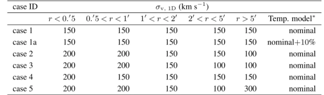
Table 4. Assumed velocity field of the one-component velocity (σv) in our simulation withGeant4. case ID σv, 1D(km s−1) r < 0.′_{5 0.}′_{5 < r < 1}′ ₁′_{< r < 2}′ ₂′_{< r < 5}′ _{r > 5}′ Temp. model∗ case 1 150 150 150 150 150 nominal case 1a 150 150 150 150 150 nominal+10% case 2 200 200 150 150 100 nominal case 3 200 200 150 100 100 nominal case 4 200 150 150 150 150 nominal case 5 200 200 150 100 300 nominal

∗_{Assumed “nominal” temperature model as shown in figure 7. We estimate the temperature}

uncertainties changing the temperature by +10% which is corresponding to the azimuthal dependence of the temperature profile from Chandra and XMM.

Fig. 9. Left: Photon lists generated by the Geant4 simulator assuming a uniform σvprofile of 150 km s−1(case 1) for the inner, 0.′5(radius), region in Perseus

(top panel). Red and black lines correspond to simulations with and without RS, respectively. Right: mock spectra for the obs23 cen region with the HEAsim tool with the photon lists generated by the Geant4 simulator. Small panels show a zoom-in around the FeXXVHeα complex. The suppression of the w line in the simulated spectra is consistent with the previous results by Zhuravleva et al. (2013).

simulated incident spectrum from the inner0.′_{5 radius of the}

cluster for a uniformσvof 150 km s−1(case 1 in table 4). The

bottom panel of the figure shows the ratio of the photon lists for the models with and without RS. Thew line flux is obvi-ously suppressed by the RS effect. Note that the suppressedw line shape is not represented by a Gaussian model which has the sameσ as the w line without RS. The suppression of the w line in our simulation agrees with previous results by Zhuravleva et al. (2013). On the other hand, the predicted line broaden-ings due to the distortion with the Geant4 simulator are slightly wider than those from ICMMC. However, the difference is quite negligible after smoothed by the Hitomi responses as described in the next paragraph.

After generating the projected photon lists with the Geant4 simulator, we processed them with the HEAsim software in Ftools to make mock event files for the Hitomi SXS FOV, tak-ing into account the Hitomi responses. The HEAsim software calculates the redistribution of the input photons, including the Hitomi mirror and detector responses such as the effective area, the PSF, and the energy resolution. Here, we used the responses

in the HEAsim tools and normalized the flux to the observed value, taking into account events out of the SXS FOV. We as-sumed a 1 Ms exposure time for each simulation. Black and red spectra in the right panel of figure 9 show the mock spectra for obs23 cen with and without RS, respectively, for the 150 km s−1 _uniformσ

v (case 1) model. One can clearly see the flux

suppression in thew line when RS is taken into account. As shown in the bottom panels in figure 9, the resonance line shape are clearly distorted by the line broadening as well as the line suppression in the mock spectrum. Note that the mock spec-tra have finite numbers of photons since the mock specspec-tra are normalized to a given, finite flux.

To estimate the potential impact of systematic uncertainties in the input model, we also performed simulations with the tem-perature and abundance profiles of the input model changed by +10% (case 1a), and ±10%, respectively. Also, we explored the effects of the moving core within 1′_{, with 150 km s}−1 _in

redshift relatively against the surrounding gas, as pointed out in “V” paper (Hitomi collaboration et al. 2017d).

5.4 Monte Carlo simulations with the ICMMC code In order to interpret the observed resonance line suppression and infer velocities of gas motions, we also applied a different approach, based on Monte Carlo simulations of radiative trans-fer in hot gas described in Zhuravleva et al. (2010) (see also Sazonov et al. 2002; Churazov et al. 2004). Here, instead of simulating the whole spectrum and fitting it with plasma mod-els to obtain line ratios, we performed calculations in specific lines. Such simulations directly provide fluxes in the considered lines for models with and without RS; their ratios, corrected for the PSF, are then compared with the observed values. This ap-proach has been successfully applied to the analysis of RS and velocity measurements in massive elliptical galaxies and galaxy groups (Werner et al. 2009; de Plaa et al. 2012; Ogorzalek et al. 2017). In these previous works the detailed treatment of indi-vidual interactions in the simulations is described.

Since the Hitomi measurements of line broadening and vari-ations of line centroids do not show strong radial velocity gra-dients in the Perseus Cluster, and the properties of the velocity field outside the inner ∼ 100 kpc are unknown, we conserva-tively assume that the velocity of gas motions is approximately the same within the considered regions. The simulations are done for a grid of characteristic velocity amplitudes, the results of which are then compared with the observed line ratios (see section 6.2).

6 Comparisons of the observed line ratios

and the simulations

6.1 GEANT4 simulations

We compared the spatial distribution of the observed line ratios with the simulations described in section 5.3. In order to com-pare the line ratios and widths, we fitted the simulated spectra with the same spectral model and responses for the ICM dis-cussed in section 4, i.e. the “modified” bvvapec (bvvapec with the strongest lines deleted) plus Gaussian models. The mock spectra are well represented by this model. To understand the impact of limited photon statistics in the modeling, we divided the simulated event list into ten 100 ks parts, each of which had similar statistics in FeXXVHeα to the observed Hitomi data.

Figure 5 shows comparisons of the observed and predicted line ratios and widths, andσvfor case 1 (flatσvfield), with and

without RS. The observed ratios of the FeXXVHeα w/z are consistent with those from simulation with RS. The simulated ratios without RS, shown by light gray diamonds, are clearly far away from the observed ones in the inner regions. Figure 10 shows the comparisons for all models listed assuming a plausi-ble velocity field based on the “V” paper (Hitomi collaboration et al. 2017d) in table 4. For all the regions, simulations of the w/z ratio for all the cases are broadly consistent with the ob-servations as shown in figures 5 and 10. The observed widths

of thew and z lines for the central region obs23 cen and the obs1 whole are well represented by the simulation with RS for cases 1, 4, and 5. The simulation for case 4 which is close to the line-of-sight velocity dispersion field in the “V” paper agrees well with the observed line ratios and widths. The simulated line widths with RS for case 2 look slightly broader than the ob-served one, while simulations with lowerσv(< 100 km s−1) in

r > 2′

, such as case 3, are poorly described in the outer regions. Consequently, our simulation assuming plausible velocity field based on the “V” paper is consistent with the observation, while the constant distribution and the relatively largeσvof ∼ 300 km

s−1_{at large radius would not be rejected from our simulation.}

The simulations show that the predicted line ratios and widths are affected by the assumed velocity field rather than the RS ef-fects. For the obs23 out region which includes the north-west ’ghost’ bubble as shown in the “V” paper, the line widths from simulations are broader than observations due to the azimuthal dependence.

As for thew/Heβ, w/Lyα1, andw/Lyα2 lines, the

simu-lated ratios with the RS effects also broadly agree with the ob-served ones within the statistical errors, except forw/Lyα1in

the obs23 out and obs1 whole regions. The Lyα line ratios are sensitive to the azimuthal dependence and hotter component of projected temperature. On the other hand, the observedz/Heβ ratios, whose lines have low optical depth than the other lines as shown in figure 8, are also consistent with the simulated ratios.

The temperatures derived from the simulated spectra are lower than the observed ones for all the regions. It should be noted that thew/z line ratio does not change much even if the temperature andσv+thchange. In fact, changing the

temper-ature in simulations by+10% for case 1a, which corresponds to the azimuthal scattering, does not change the results within the observed statistical errors. The derived σvfor cases 1, 4

and 5 agree well with the observations in the innermost region, while those in the obs23 out region are lower than the simu-lated ones. We also estimated the uncertainties by changing the Fe abundance by ±10%. The resultant line ratios do not change by more than ∼ 3%.

In this simulation, we assumed spherical symmetry in the cluster core. If bulk motion existed along the line of sight in the cluster core, the line widths should be broader along line of sight. The “V” paper (Hitomi collaboration et al. 2017d) actu-ally shows a large scale bulk velocity gradient of ∼ 100 km s−1_.

As shown in section 4, we adopted the gain correction, which gave ∼ 5% broader line widths than the uncorrected data, but the “V” paper did not. In order to estimate the uncertainties, we performed simulations with the assumption of the core moving within0.′_{5 radius with 150 km s}−1_{relative to the surrounding}

gas based on case 1. The resultantw/z line ratios in obs23 cen did not change within the statistical errors for case1. Therefore, we confirmed that the RS effect is not very sensitive to bulk