U
NIVERSITÀ DELLA
C
ALABRIA
Dipartimento di Elettronica,
Informatica e Sistemistica
Dottorato di Ricerca in
Ingegneria dei Sistemi e Informatica
XIX ciclo
Tesi di Dottorato
Swarm-Based Algorithms for
Decentralized Clustering and
Resource Discovery in Grids
Agostino Forestiero
Acknowledgments
I wish to express my sincere gratitude to my thesis advisor Ing. Giandomenico Spezzano for guiding me through every step of the thesis and providing me direction and insight on numerous occasions during the course of this work. I would like to thank my colleagues (friends) Ing. Gianluigi Folino and Ing. Carlo Mastroianni for their precious support and patience. Special thanks go to my parents and my brother Francesco. I would also like to thank my wife, Sara, for her loving support and appreciation. Moreover, I cannot forget to thank my friends and colleagues at ICAR-CNR institute, in particularly Giuseppe Papuzzo and Oreste Verta.
Contents
1 Introduction. . . 1
1.1 Background and Motivations . . . 1
1.2 Main Contributions of the Thesis . . . 2
1.3 Thesis Organization . . . 3
2 Swarm-Based Systems. . . 5
2.1 Introduction . . . 5
2.2 Self-Organization . . . 7
2.2.1 Stigmergy . . . 7
2.3 Foraging behavior of ants . . . 10
2.3.1 Ant colony optimization . . . 11
2.4 Particle swarm optimization . . . 12
2.5 Multiagent Systems . . . 13
3 Approximate Clustering by Adaptive Flock. . . 17
3.1 Introduction . . . 17
3.2 Flocking algorithm . . . 19
3.2.1 The Reynolds’ model . . . 20
3.2.2 Searching objects in spatial data . . . 20
3.3 Clustering spatial data . . . 24
3.3.1 The DBSCAN algorithm . . . 24
3.3.2 SPARROW algorithm . . . 25 3.3.3 The SNN algorithm . . . 26 3.3.4 SPARROW-SNN algorithm . . . 27 3.4 Experimental results . . . 28 3.4.1 SPARROW results . . . 28 3.4.2 SPARROW-SNN results . . . 33 3.5 Entropy model . . . 39 3.5.1 Spatial Entropy . . . 39 3.5.2 Autocatalytic property . . . 41 3.6 Related works . . . 43
4 P2P clustering algorithm . . . 47
4.1 Introduction . . . 47
4.2 P-Sparrow . . . 48
4.2.1 Density-based clustering . . . 48
4.2.2 Distributed clustering . . . 49
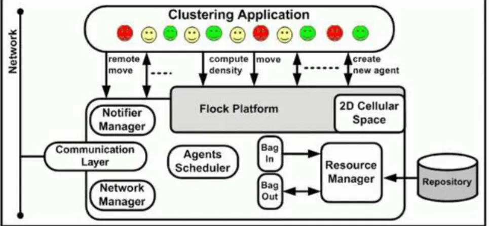
4.2.3 The software architecture . . . 51
4.3 Experimental Results . . . 52
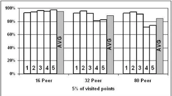
4.3.1 Accuracy and Scalability . . . 52
4.3.2 The impact of Small World topology . . . 56
5 An Ant-Inspired Protocol for Mapping Resources in Grid . 59 5.1 Introduction . . . 59 5.2 ARMAP protocol . . . 60 5.3 Basic operations . . . 61 5.3.1 Agent Movement . . . 61 5.3.2 Pick operation . . . 61 5.3.3 Drop operation . . . 62 5.3.4 Dynamic Grid . . . 62
5.4 Spatial entropy and pheromone mechanism . . . 63
5.4.1 Design of P2P information systems in Grids . . . 65
5.5 Protocol Analysis . . . 66
5.5.1 Simulation Parameters and Performance Indices . . . 66
5.6 Protocol modality . . . 67
5.7 Number and mobility of agents . . . 70
5.8 Number of classes and network size . . . 73
5.9 Related Work . . . 77
6 Discovering Categorized Resources in Grids . . . 81
6.1 Introduction . . . 81
6.2 Identification of representative peers . . . 81
6.3 Semi-informed search . . . 82
6.4 Stigmergy mechanism . . . 82
6.5 Protocol Analysis . . . 84
6.5.1 Description of the environment . . . 84
6.5.2 Performance . . . 86
7 Conclusions & Future Works . . . 97
1
Introduction
1.1 Background and Motivations
In recent times, distributed computing has considerably changed due to new developments of information technology. New environments has emerged such as massively large-scale, wide-area computer networks and mobile ad-hoc net-works. These environments represent an enormous potential for future appli-cations: they enable communication, storage, and computational services to be built in a bottom-up fashion (e.g. peer-to-peer system and Grid Computing). However, these environments present a few problems because they can be extremely dynamic and unreliable. Traditional approaches to the design of distributed systems which assume reliable components or based on central and explicit control are not applicable for these environments. Furthermore, central control introduces a single-point-of-failure which should be avoided whenever possible [4]. In order to tackle these issues, an artificial intelli-gence technique based on the study of collective behavior in decentralized, self-organized systems, namely Swarm Intelligence [7], appears particularly suitable. Swarm Intelligence systems are typically made up of a population of simple agents interacting locally with one another and with their environment. Although there is normally no centralized control structure dictating how in-dividual agents should behave, local interactions between such agents often lead to the emergence of global behavior. Examples of systems like these can be found in nature, including ant colonies, bird flocking, animal herding, bac-teria molding and fish schooling. Swarms offer several advantages compared to traditional systems:
- robustness, - flexibility, - scalability, - adaptability,
Simple agents are less likely to fail than more complex ones. If they do fail, they can be pulled out entirely or replaced without significantly impacting the overall performance of the system. Distributed systems are therefore, tolerant of agent error and failure. They are also highly scalable: increasing the number of agents or task size does not greatly affect performance. The inherent par-allelism and scalability make the swarm-based algorithms very suitable to be used in environment whose structure dynamically changes. In systems using central control, the high communications and computational costs required to coordinate agent behavior limit the size of the system to at most a few dozen agents. The simplicity of agent’s interactions with other agents make swarms amenable to quantitative mathematical analysis. There are multiple examples of complex collective behavior among social insects: trail formation in ants, hive building by bees and mound construction by termites are just few examples. The apparent success of these organisms has inspired computer scientists and engineers to design algorithms and distributed problem-solving systems modelled after them [8], especially for systems which are characterized by decentralized control, large scale and extreme dynamism of their operating environment as peer-to-peer system, Grid Computing, etc..
1.2 Main Contributions of the Thesis
In this thesis, some novel algorithms based on swarm intelligent paradigm are proposed. In particular, the swarm agents, was exploited to tackle the following issues:
- P2P Clustering. A swarm-based algorithm is used to cluster distributed data in a peer-to-peer environment through a small worlds topology. More-over, to perform spatial clustering in every peer, two novel algorithms are proposed. They are based on the stochastic search of the flocking algo-rithm and on the main principles of two popular clustering algoalgo-rithms, DBSCAN and SNN.
- Resource discovery in Grids. An approach based on ant systems is
exploited to replicate and map Grid services information on Grid hosts according to the semantic classification of such services. To exploit this mapping, a semi-informed resource discovery protocol which makes use of the ants’ work has been achieved. Asynchronous query messages (agents) issued by clients are driven towards ”representative peers” which main-tain information about a large number of resources having the required characteristics.
1.3 Thesis Organization 3
1.3 Thesis Organization
The thesis organized as follows:
Chapter 2 I present some of the critical notions of Swarm Intelligence and the research work that has addressed them. These notions, organized around the concept of problem-solving which is one of the most overall character-istics that an SI exhibits.
Chapter 3 presents an adaptive flocking algorithm based on the biology-inspired paradigm of a flock of birds. We used swarming agents (SA), i.e. a population of simple agents interacting locally with each other and with the environment. They provide models of distributed adaptive orga-nization and they are useful to solve difficult optimization, classification, distributed control problems, etc...
Chapter 4 describes P-SPARROW, a algorithm for distributed clustering of data in peer-to-peer environments combining a smart exploratory strategy based on a flock of birds with a density-based strategy to discover clusters of arbitrary shape and size in spatial data.
Chapter 5 shows as an Ant-based Replication and MApping Protocol (ARMAP) is used to disseminate resource information by a decentralized mechanism, and its effectiveness is evaluated by means of an entropy in-dex. Information is disseminated by agents - ants - that traverse the Grid by exploiting P2P interconnections among Grid hosts. A mechanism in-spired by real ants’ pheromone is used by each agent to autonomously drive its behavior on the basis of its interaction with the environment. Chapter 6 proposes a semi-informed discovery protocol (namely ARDIP,
Ant-based Resource DIscovery Protocol) to exploit the logical resource orga-nization achieved by ARMAP.
2
Swarm-Based Systems
2.1 Introduction
The term Swarm, in a general sense, refers to any such loosely structured collection of interacting agents. The classic example of a swarm is a swarm of bees, but the metaphor of a swarm can be extended to other systems with a similar architecture. An ant colony can be thought of as a swarm whose individual agents are ants, a flock of birds is a swarm whose agents are birds, traffic is a swarm of cars, a crowd is a swarm of people, an immune system is a swarm of cells and molecules, and an economy is a swarm of economic agents. A high-level view of a swarm suggests that the N agents in the swarm are cooperating to achieve some goal. This apparent collective intelligence seems to emerge from what are often large groups of relatively simple agents. The agents use simple local rules to govern their actions and via the interactions of the entire group, the swarm achieves its objectives. A type of self-organization emerges from the collection of actions of the group. Swarm intelligence is the emergent collective intelligence of groups of simple autonomous agents. Here, an autonomous agent is a subsystem that interacts with its environment, which probably consists of other agents, but acts relatively independently from all other agents. The autonomous agent does not follow commands from a leader, or some global plan.
For example, for a bird to participate in a flock, it only adjusts its move-ments to coordinate with the movemove-ments of its flock mates, typically its neigh-bors that are close to it in the flock. A bird in a flock simply tries to stay close to its neighbors, but avoid collisions with them. Each bird does not take com-mands from any leader bird since there is no lead bird. Any bird can fly in the front, center and back of the swarm. Swarm behavior helps birds take ad-vantage of several things including protection from predators (especially for birds in the middle of the flock), and searching for food (essentially each bird is exploiting the eyes of every other bird). Researchers try to examine how collections of animals, such as flocks, herds and schools, move in a way that appears to be orchestrated. In 1987, Reynolds created a boid model, which
Fig. 2.1. Reynolds showed that a realistic bird flock could be programmed by im-plementing three simple rules: match your neighbors velocity, steer for the perceived center of the flock, and avoid collisions.
is a distributed behavioral model, to simulate on a computer the motion of a flock of birds [103] (see in Fig. 2.1). Each boid is implemented as an inde-pendent actor that navigates according to its own perception of the dynamic environment. A boid must observe the following rules. A boid must:
- move away from boids that are too close; - follows direction and velocity of the flock; - move towards boids that are too distant.
The swarm behavior of the simulated flock is the result of the dense interaction of the relatively simple behaviors of the individual boids. Swarm robotics is currently one of the most important application areas for swarm intelligence. Swarms provide the possibility of enhanced task performance, high reliabil-ity (fault tolerance), low unit complexreliabil-ity and decreased cost over traditional robotic systems. They can accomplish some tasks that would be impossible for a single robot to achieve. Swarm robots can be applied to many fields, such as flexible manufacturing systems, spacecraft, inspection/maintenance, construction, agriculture, and medicine work [7].
2.2 Self-Organization 7
2.2 Self-Organization
Self-Organization is a set of dynamical mechanism whereby structures appear at the global level of system from interactions among its lower-level compo-nents. The rules specifying the interactions among the system’s constituent unit are executed on the basis of purely local information, without reference to the global pattern, which is an emergent property of the system rather than a property imposed upon the system by an external ordering influence. For example, the emerging structures in the case of foraging in ants include spa-tiotemporally organized networks of pheromone trails. Self-organization relies on four basic ingredients:
- Positive feedback amplifies a certain behavior, e.g. bees may recruit other bees to follow them to good food sources.
- Negative feedback on the other hand limits a behavior, e.g. if a food source is too crowded.
- The amplification of fluctuations enables discovery of a new collective be-havior resulting from random walks or errors of individuals.
- Multiple interactions between individuals are necessary for a new behavior to be adopted by the swarm.
When a given phenomenon is self-organized, it can usually be characterized by a few properties:
1. The creation of spatiotemporal structures in an initially homogeneous medium. Such structures include nest architectures, foraging trail, or so-cial organization. For example, a characteristic well-organized pattern de-velops on the combos honeybee colonies, i.e. three concentric regions. 2. The possible coexistence of several stable states (multistability). Because
structures emerge by amplification of random deviations, any such devi-ation can be amplified, and the system converges to one among several possible stable state, depending on initial conditions.
3. The existence of bifurcations when some parameters are varied. The be-havior of a self-organized system changes dramatically at bifurcations. 2.2.1 Stigmergy
Self-Organization in social insect often required interactions among insect: such interactions can be direct or indirect. Direct interactions are the ”obvi-ous” interactions: antennation, trophallaxis (food or liquid exchange), mandibu-lar contact, visual contact, chemical contact (the odor of nearby nestmates), etc. Indirect interactions are more suitable: two individuals interact indirectly when one of them modifies the environment and the other respond to the new environment at a later time. The indirect form of communication among individuals was first described by French entomologist Pierre-Paul Grass in the 1950s and denominated stigmergy (from the Greek sigma: sting and er-gon: work) [40]. Stigmergy has helped researchers understand the connection
between individual and collective behaviour. The basic principle of stigmergy is extremely simple:
- Traces left and modifications made by individuals in their environment may feed back on them.
The colony records its activity in part in the physical environment and uses this record to organize the collective behaviour. Various forms of storage are used:
- gradients of pheromones; - material structures;
- spatial distribution of colony elements.
Such structures materialize the dynamics of the colonys collective behaviour and constrain the behaviour of the individuals through a feedback loop. Hol-land and Beckers distinguish between cue-based and sign-based stigmergy. In cue-based stigmergy, the change in the environment simply provides a cue for the behavior of other actors, while in sign-based stigmergy the environmental change actually sends a signal to other actors. Termite arch-building contains both kinds of stigmergy, with pheromones providing signals while the growing pillars provide cues. Ant corpse-piling has been described as a cue-based stig-mergic activity. When an ant dies in the nest, the other ants ignore it for the first few days, until the body begins to decompose. The release of chemicals related to oleic acid stimulates a passing ant to pick up the body and carry it out of the nest. Some species of ants actually organize cemeteries where they deposit the corpses. If dead bodies of these species are scattered randomly over an area, the survivors will hurry around picking up the bodies, moving them, and dropping them again, until soon all the corpses are arranged into a small number of distinct piles. The piles might form at the edges of an area or on a prominence or other heterogeneous feature of the landscape. Deneubourg [24] have shown that ant cemetery formation can be explained in terms of sim-ple rules. The essence of the rule set is that isolated items should be picked up and dropped at some other location where more items of that type are present. A similar algorithm appears to be able to explain larval sorting, in which larvae are stored in the nest according to their size, with smaller larvae near the center and large ones at the periphery, and also the formation of piles of woodchips by termites. In the latter, termites may obey the following rules:
- If you are not carrying a woodchip and you encounter one, pick it up. - If you are carrying a woodchip and you encounter another one, set yours
down.
Thus a woodchip that has been set down by a termite provides a stigmergic cue for succeeding termites to set their woodchips down. If a termite sets a chip down where another chip is, the new pile of two chips becomes proba-bilistically more likely to be discovered by the next termite that comes past
2.2 Self-Organization 9
carrying a chip, since its bigger. Each additional woodchip makes the pile more conspicuous, increasing its growth more and more in an autocatalytic loop. Stigmergy alone is not sufficient to explain collective intelligence, as it only refers to animal-animal interactions. Therefore, it has to be complemented with an additional mechanism that makes use of these interactions to coor-dinate and regulate the collective task in a particular way. One of the best examples of this mechanism was studied by Grass: the building behaviour of termites. Grass showed that the coordination and regulation of building ac-tivities do not depend on the workers themselves but are mainly achieved by the nest structure: A stimulating configuration triggers a building action of a termite worker, transforming the configuration into another configuration that may trigger in turn another (possibly different) action performed by the same termite or any other termite in the colony. The use of stigmergy is not confined to building structures. It also occurs in cooperative foraging strate-gies such as trail recruitment in ants, where the interactions between foragers are mediated by pheromones put on the ground in quantities determined by the local conditions of the environment. For example, trail recruitment in ant species are able to select and preferentially exploit the richest food source in the neighbourhood or the shortest path between the nest and a food source: foragers are initially evenly distributed between the two sources, but one of the sources randomly becomes slightly favoured, and this difference may be amplified by recruitment, since the more foragers there are at a given source, the more individuals recruited to that source . Michener describes in [85] many activities in bee colonies that result in nest structures, conditions of brood or stored food, to which other bees respond. Referring to this as indirect social interactions, where the construct is made for other primary objectives, not for signalling, although the information content becomes essential for colony integration. In nectar source decision making in honey bees it is less clear if only direct communication through the recruitment dances of the bees pro-duce the self-organizing behaviour, or if also the indirect communication given by the waiting time for downloading the honey is affecting the collective be-haviour [108]. As a consequence of stigmergy and self-organization, complex behaviours which had been explained on the basis of certain rules of interac-tion among individuals were later accounted for even simpler behaviours in the context of environmental stimuli. Stigmergy seems indeed at the root of several collective behaviours of social insects, especially in their building activ-ities. This is certainly a powerful principle, as social insect constructions are remarkable for their complexity, size and adaptive value. However, it is possi-ble to extend the idea easily to other domains; it can be seen as an even more impressive and general account of how simple systems can produce a range of apparently highly organized and coordinated behaviours and behavioural outcomes, simply by exploiting the influence of the environment.
2.3 Foraging behavior of ants
Ant colony expresses a complex collective behavior providing intelligent solu-tions to problems such as carrying large items, forming bridges and finding the shortest routes from the nest to a food source. A single ant has no global knowledge about the task it is performing. The ant’s actions are based on local decisions and are usually unpredictable. The intelligent behavior natu-rally emerges as a consequence of the self-organization and indirect commu-nication between the ants. This is what is usually called Emergent Behavior or Emergent Intelligence. Ants use a signaling communication system based on the deposition of pheromone over the path it follows, marking a trail. Pheromone is a hormone produced by ants that establishes a sort of indirect communication among them. Basically, an isolated ant moves at random, but when it finds a pheromone trail there is a high probability that this ant will decide to follow the trail. An ant foraging for food lay down pheromone over its route. When this ant finds a food source, it returns to the nest reinforcing its trail. Pheromone evaporates with passing of the time with evaporation rate Ev (see formula 2.1).Other ants in the proximities are attracted by this sub-stance and have greater probability to start following this trail and thereby laying more pheromone on it.
Φ= Ev ∗ Φi−1+ φi (2.1)
This process works as a positive feedback loop system because the higher the intensity of the pheromone over a trail, the higher the probability of an ant start traveling through it.This elementary behavior of real ants can be used to explain how they can find the shortest path which reconnects a broken line after the sudden appearance of an unexpected obstacle has interrupted the initial path (see Fig. 2.2). In fact, once the obstacle has appeared, those ants which are just in front of the obstacle cannot continue to follow the pheromone trail and therefore they have to choose between turning right or left. In this situation we can expect half the ants to choose to turn right and the other half to turn left. The very same situation can be found on the other side of the obstacle. It is interesting to note that those ants which choose, by chance, the shorter path around the obstacle will more rapidly reconstitute the interrupted pheromone trail compared to those which choose the longer path. Hence, the shorter path will receive a higher amount of pheromone in the time unit and this will in turn cause a higher number of ants to choose the shorter path. Due to this positive feedback (autocatalytic) process, very soon all the ants will choose the shorter path. The most interesting aspect of this autocatalytic process is that finding the shortest path around the obstacle seems to be an emergent property of the interaction between the obstacle shape and ants distributed behavior: Although all ants move at approximately the same speed and deposit a pheromone trail at approximately the same rate, it is a fact that it takes longer to contour obstacles on their longer side than on their shorter side which makes the pheromone trail accumulate quicker on the shorter side.
2.3 Foraging behavior of ants 11
Fig. 2.2. Pheromones accumulate on the shorter path because any ant that sets out on that path returns sooner.
It is the ants preference for higher pheromone trail levels which makes this accumulation still quicker on the shorter path.
2.3.1 Ant colony optimization
”Ant colony optimization” [8] is based on the observation that ants will find the shortest path around an obstacle separating their nest from a target such as a piece of candy simmering on a summer sidewalk. As ants move around they leave pheromone trails, which dissipate over time and distance. The pheromone intensity at a spot, that is, the number of pheromone molecules that a wandering ant might encounter,is higher either when ants have passed over the spot more recently or when a greater number of ants have passed over the spot. Thus ants following pheromone trails will tend to congregate simply from the fact that the pheromone density increases with each additional ant that follows the trail. Ants meandering from the nest to the candy and back will return more quickly, and thus will pass the same points more frequently, when following a shorter path. Passing more frequently, they will lay down a denser pheromone trail. As more ants pick up the strengthened trail, it be-comes increasingly stronger (see in Fig. 2.2). In computer adaptation of these behaviors [8] let a population of ”ants” search a traveling salesman map sto-chastically, increasing the probability of following a connection between two
cities as a function of the number of other simulated ants that had already followed that link. By exploitation of the positive feedback effect, that is, the strengthening of the trail with every additional ant, this algorithm is able to solve quite complicated combinatorial problems where the goal is to find a way to accomplish a task in the fewest number of operations. Research on live ants has shown that when food is placed at some distance from the nest, with two paths of unequal length leading to it, they will end up with the swarm follow-ing the shorter path. If a shorter path is introduced, though, for instance, if an obstacle is removed, they are unable to switch to it. If both paths are of equal length, the ants will choose one or the other. If two food sources are offered, with one being a richer source than the other, a swarm of ants will choose the richer source; if a richer source is offered after the choice has been made, most species are unable to switch, but some species are able to change their pat-tern to the better source. If two equal sources are offered, an ant will choose one or the other arbitrarily.The movements of ants are essentially random as long as there is no systematic pheromone pattern; activity is a function of two parameters, which are the strength of pheromones and the attractiveness of the pheromone to the ants. If the pheromone distribution is random, or if the attraction of ants to the pheromone is weak, then no pattern will form. On the other hand, if a too-strong pheromone concentration is established, or if the attraction of ants to the pheromone is very intense, then a subop-timal pattern may emerge, as the ants crowd together in a sort of pointless conformity. In real and simulated examples of insect accomplishments, we see optimization of various types, whether clustering items or finding the shortest path through a landscape, with certain interesting characteristics. None of these instances include global evaluation of the situation: an insect can only detect its immediate environment. Optimization traditionally requires some method for evaluating the fitness of a solution, which seems to require that candidate solutions be compared to some standard, which may be a desired goal state or the fitness of other potential solutions.
2.4 Particle swarm optimization
Particle swarm optimization (PSO) was originally developed by Eberhart and Kennedy in 1995 [64]. It is a global optimization algorithm for dealing with problems in which a best solution can be represented as a point or surface in an n-dimensional space. Hypotheses are plotted in this space and seeded with an initial velocity, as well as a communication channel between the particles. Particles then move through the solution space, and are evaluated according to some fitness criterion after each timestep. Over time, particles are acceler-ated towards those particles within their communication grouping which have better fitness values. The main advantage of such an approach over other global minimization strategies such as simulated annealing is that the large number of members that make up the particle swarm make the technique
2.5 Multiagent Systems 13
impressively resilient to the problem of local minima. PSO was inspired by the social behavior of a flock of birds. In the PSO algorithm, the birds in a flock are symbolically represented as particles. These particles can be consid-ered as simple agents ”flying” through a problem space. A particles location in the multi-dimensional problem space represents one solution for the prob-lem. When a particle moves to a new location, a different problem solution is generated. This solution is evaluated by a fitness function that provides a quantitative value of the solutions utility. The velocity and direction of each particle moving along each dimension of the problem space will be altered with each generation of movement. In combination, the particles personal ex-perience, Pid and its neighbors’ experience, Pgd influence the movement of
each particle through a problem space. The random values rand1and rand2
are used for the sake of completeness, that is, to make sure that particles explore a wide search space before converging around the optimal solution. The values of c1 and c2control the weight balance of Pid and Pgd in deciding
the particles next movement velocity. At every generation, the particles new location is computed by adding the particles current velocity, vid, to its
loca-tion, xid. Mathematically, given a multi-dimensional problem space, the ith
particle changes its velocity and location according to the following equations [64]:
vid = w ∗ vid+ c1∗ rand1∗ (pid− xid) + c2 ∗ rand2∗ (pgd− xid) (2.2)
xid= xid+ vid (2.3)
where w denotes the inertia weight factor; pidis the location of the particle
that experiences the best fitness value; pgd is the location of the particles that
experience a global best fitness value; c1 and c2 are constants and are known
as acceleration coefficients; d denotes the dimension of the problem space; rand1, rand2are random values in the range of (0, 1).
2.5 Multiagent Systems
Multiagent systems are computational systems in which two or more agents interact or work together to perform some set of tasks or to satisfy some set of goals. These systems may be comprised of homogeneous or heterogeneous agents. An agent in the system is considered a locus of problem-solving ac-tivity, it operates asynchronously with respect to other agents, and it has a certain level of autonomy. Agent autonomy relates to an agents ability to make its own decisions about what activities to do, when to do them, what type of information should be communicated and to whom, and how to assimilate the information received. Autonomy can be limited by policies built into the
agent by its designer, or as a result of an agent organization dynamically com-ing to an agreement that specific agents should take on certain roles or adopt certain policies for some specified period. Closely associated with agent au-tonomy is agent adaptability the more auau-tonomy an agent possesses the more adaptable it is to the emerging problem solving and network context. The degree of autonomy and the range of adaptability are usually associated with the level of intelligence/sophistication that an agent possesses. Agents may also be characterized by whether they are benevolent (cooperative) or self-interested. Cooperative agents work toward achieving some common goals, whereas self-interested agents have distinct goals but may still interact to advance their own goals. In the latter case, self-interested agents may, by exchanging favors or currency, coordinate with other agents in order to get those agents to perform activities that assist in the achievement of their own objectives. For example, in a manufacturing setting where agents are respon-sible for scheduling different aspects of the manufacturing process, agents in the same manufacturing company would behave in a cooperative way while agents representing two separate companies where one company was outsourc-ing part of its manufacturoutsourc-ing process to the other company would behave in a selfinterested way. Scientific research and practice in multiagent systems, which in the past has been called Distributed Artificial Intelligence (DAI), focuses on the development of computational principles and models for con-structing, describing, implementing and analyzing the patterns of interaction and coordination in both large and small agent societies. Multiagent systems research brings together a diverse set of research disciplines and thus there is a wide range of ideas currently being explored. Multiagent systems over the past few years have come to be perceived as crucial technology not only for effectively exploiting the increasing availability of diverse, heterogeneous, and distributed on-line information sources, but also as a framework for building large, complex, and robust distributed information processing systems which exploit the efficiencies of organized behavior. Multiagent systems also provide a powerful model for computing , in which networks of interacting, real-time, intelligent agents seamlessly integrate the work of people and machines, and dynamically adapt their problem solving to effectively deal with changing us-age patterns, resource configurations and available sources of expertise and information. Application domains in which multiagent system technology is appropriate typically have a naturally spatial, functional or temporal decom-position of knowledge and expertise. By structuring such applications as a multiagent system rather than as a single agent, the system will have the following advantages:
- speed-up due to concurrent processing;
- less communication bandwidth requirements because processing is located nearer the source of information;
2.5 Multiagent Systems 15
- improved responsiveness due to processing, sensing and effecting being co-located;
- easier system development due to modularity coming from the
decompo-sition into semiautonomous agents.
Examples of application domains that have used a multiagent approach in-clude:
- Distributed situation assessment, which emphasizes how (diagnostic) agents with different spheres of awareness and control (network segments) should share their local interpretations to arrive at consistent and comprehen-sive explanations and responses (e.g., network diagnosis [112]; information gathering on the Internet [22] [92]; distributed sensor networks [13].
- Distributed resource scheduling and planning, which emphasizes how
(scheduling) agents (associated with each work cell) should coordinate their schedules to avoid and resolve conflicts over resources, and to max-imize system output (e.g., factory scheduling [90]; network management [2]; and intelligent environments [50]).
- Distributed expert systems, which emphasize how agents share informa-tion and negotiate over collective soluinforma-tions (designs) given their different expertise and solution criteria (e.g., concurrent engineering [72]; network service restoral [55]).
The next generation of applications will integrate characteristics of each of these generic domains. The need for a multiagent approach can also come from applications in which agents represent the interests of different orga-nizational entities (e.g., electronic commerce and enterprise integration [6]). Other emerging uses of multiagent systems are in layered systems architec-tures in which agents at different layers need to coordinate their decisions (e.g., to achieve appropriate configurations of resources and computational processing), and in the design of survivable systems in which agents dynam-ically reorganize to respond to changes in resource availability, software and hardware malfunction, and intrusions. In general, multiagent systems provide a framework in which both the inherent distribution of processing and infor-mation in an application and the complexities that come from issues of scale can be handled in a natural way [74]. There are two ways in order to design the multi-agent systems :
- the traditional paradigm, based on deliberative agents and (usually) cen-tral control;
- the swarm paradigm, based on simple agents and distributed control; In the past, researchers in the Artificial Intelligence and related communities have, for the most part, operated within the first paradigm. They focused on making the individual agents, be they software agents or robots, smarter and more complex by giving them the ability to reason, negotiate and plan action. In these deliberative systems complex tasks can be done either in-dividually or collectively. If collective action is required to complete some
task, a central controller is often used to coordinate group behavior. Swarm Intelligence represents an alternative approach to the design of multi-agent systems. Swarms are composed of many simple agents. These systems are self-organizing, meaning collective behavior emerges from local interactions among agents and between agents and the environment, there is no central controller.
3
Approximate Clustering by Adaptive Flock
3.1 Introduction
Clustering data is the process of grouping similar objects according to their distance, connectivity, or relative density in space [44]. There are a large num-ber of algorithms for discovering natural clusters in a data set, but they are usually implemented in a centralized way. These algorithms can be classi-fied into partitioning methods [62], hierarchical methods [61], density-based methods [105], grid-based methods [123]. Han, Kamber and Tung’s paper [45] is a good introduction to this subject. Many of these algorithms work on data contained in a file or database. In general, clustering algorithms focus on creating good compact representation of clusters and appropriate distance functions between data points. For this purpose, they generally need one or more parameters chosen by a user that indicate the characteristics of the ex-pected clusters. Centralized clustering is problematic if we have large data to explore or data are widely distributed. Parallel and distributed computing is expected to relieve current mining methods from the sequential bottleneck, providing the ability to scale to massive datasets, and improving the response time. Achieving good performance on today’s high performance systems is a non-trivial task. The main challenges include synchronization and communi-cation minimization, work-load balancing, finding good data decomposition, etc. Some existing centralized clustering algorithms have been parallelized and the results have been encouraging. Centralized schemes require high level of connectivity, impose a substantial computational burden, are typically more sensitive to failures than decentralized schemes, and are not scalable. Recently, innovative algorithms based on biological models [24] [70] [79] [89] have been introduced to solve the clustering problem in a decentralized fashion. These algorithms are characterized by the interaction of a large number of simple agents that sense and change their environment locally. Furthermore, they ex-hibit complex, emergent behavior that is robust with respect to the failure of individual agents. Ant colonies, flocks of birds, termites, swarms of bees etc. are agent-based insect models that exhibit a collective intelligent behavior
(swarm intelligence) [8]. SI models have many features in common with Evo-lutionary Algorithms (EA). Like EA, SI models are population-based and the system is initialized with a population of individuals (i.e., potential solutions). These individuals are then manipulated over many iteration steps by mimick-ing the social behavior of insects or animals, in an effort to find the optima in the problem space. Unlike EAs, SI models do not explicitly use evolutionary operators such as crossover and mutation. A potential solution simply ’flies’ through the search space by modifying itself according to its past experience and its relationship with other individuals in the population and the envi-ronment. In these models, the emergent collective behavior is the outcome of a process of self-organization, in which insects are engaged through their repeated actions and interaction with their evolving environment. Intelligent behavior frequently arises through indirect communication between the agents using the principle of stigmergy [40]. This mechanism is a powerful principle of cooperation in insect societies. According to this principle, an agent deposits something in the environment that makes no direct contribution to the task being undertaken but is used to influence the subsequent behavior that is task related. The advantages of SI are twofold. Firstly, it offers intrinsically dis-tributed algorithms that can use parallel computation quite easily. Secondly, these algorithms show a high level of robustness to change by allowing the solution to dynamically adapt itself to global changes by letting the agents self-adapt to the associated local changes. In this section, I present a new algorithm based on a flock of birds that move together in a complex manner using simple local rules, to explore spatial data for searching interesting ob-jects. The flocking algorithm, inspired by the principles of Macgill [81], was used to design two novel clustering algorithms based on the main principles of two popular clustering methods: DBSCAN and SNN. We consider cluster-ing as a search problem in a multi-agent system in which individuals agents have the goal of finding specific elements in the search space, represented by a large data set of tuples, by walking efficiently through this space. Our meth-ods take advantage of the parallel search mechanism a flock implies, by which if a member of a flock finds an area of interest, the mechanics of the flock will draw other members to scan that area in more detail. Our algorithms select interesting subsets of tuples without inspecting the whole search space guaranteeing a fast placing of points correctly in the clusters. We have applied this strategy as a data reduction technique to perform efficiently approximate clustering [67]. In the algorithm, each agent can use hierarchical, partitioned, density-based and grid-based clustering methods to discovery if a tuple be-longs to a cluster. Particle Swarm Optimization [64], inspired to the behavior of flocks of birds, school of fish, etc.., is a population based optimization tool, quite different from our approach. PSO consists of a swarm of particles, each of them representing the solution of an optimization problem, moving in the problem search space. At the beginning, each particle has a random position and velocity. A particle moves on the basis of its own experience (its best past position) and of the best of particles in the swarm. Note that, not differently
3.2 Flocking algorithm 19
from our model, variants of PSO consider the best of a local neighborhood instead of all the swarm. Furthermore, the best particle is an attractor for the other particles as the red birds of our algorithm are the attractors for the other birds. However, the similarities with our model ended here since our flock moves for searching representative points and merge them in order to find clusters, while each PSO particle represents itself a solution of a problem and as a consequence it is less flexible in searching clusters (see related works section for more details). Moreover, in the flock algorithm, there is a more strict interrelation, while particles only look at the best particle in the group. Then PSO does not use any repulsion force to avoid uninteresting zones, while our white agents are repulsive for the others.
To better illustrate the usefulness of the method, we present two algo-rithms: SPARROW (SPAtial ClusteRing AlgoRithm thrOugh SWarm Intel-ligence) and SPARROW-SNN (Shared Nearest-Neighbor similarity). SPAR-ROW combines the flocking algorithm with the density-based DBSCAN al-gorithm [32]. SPARROW-SNN couples the flocking alal-gorithm with a shared nearest neighbor (SNN) cluster algorithm [31] to discover clusters with differ-ing sizes, shapes and densities in noise, high dimensional data. We have built a SWARM [86] simulation of both algorithms to investigate the interaction of the parameters that characterize them.
The rest of this chapter is organized as follows. Section 3.2 presents the multi agent adaptive flocking algorithm, first introducing the classical model of Reynolds and then the modified behavioral rules of our algorithm that add an adaptive behavior. Section 3.3 shows how the stochastic search of the adaptive flocking algorithm can be used as a basis for clustering spatial data, combining our strategy respectively with DBSCAN and SNN to consti-tute the SPARROW and SPARROW-SNN algorithms. Section 3.4 presents the obtained results for both the approximate clustering algorithms. Section 3.5 presents an entropy-based model to theoretically explain the behavior of the algorithm. Finally, section 3.6 discusses some related works concerning clustering algorithms based on the Swarm Intelligence paradigm.
3.2 Flocking algorithm
In this section, we will present a multi-agent stochastic search based on a clas-sical flocking algorithm that has the advantage of being easily implementable on parallel and distributed machines and is robust compared to the failure of individual agents. We first introduce the Reynolds’ flock model that describes the standard movement rules of birds. Then, we illustrate the modified be-havioral rules of the swarm agents that, adding an adaptive behavior, make the flock more effective in searching points having some desired properties in the space.
3.2.1 The Reynolds’ model
The flocking algorithm was originally proposed by Reynolds [103] as a method for mimicking the flocking behavior of birds on a computer both for animation and as a way to study emergent behavior. Flocking is an example of emergent collective behavior: there is no leader, i.e., no global control. Flocking behavior emerges from the local interactions. In the flock algorithm each agent has direct access to the geometric description of the whole scene, but reacts only to flock mates within a certain small radius. The basic flocking model consists of three simple steering behaviors:
Separationgives an agent the ability to maintain a certain distance from others nearby. This prevents agents from crowding too closely together, al-lowing them to scan a wider area.
Cohesion supplies an agent the ability to cohere (approach and form
a group) with other nearby agents. Steering for cohesion can be computed by finding all agents in the local neighborhood and computing the average position of the nearby agents. The steering force is then applied in the direction of that average position.
Alignment gives an agent the ability to align with other nearby char-acters. Steering for alignment can be computed by finding all agents in the local neighborhood and averaging together the ’heading’ vectors of the nearby agents.
3.2.2 Searching objects in spatial data
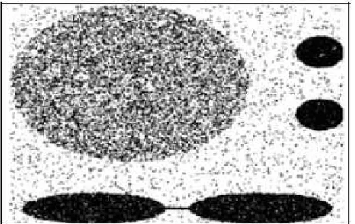
Different techniques can be used to cope with the problem of searching inter-esting object in spatial data. We introduced a multi-agent adaptive algorithm able to discover these points in parallel. Our algorithm uses a modified version of standard flocking algorithm, described above, that incorporates the capac-ity for learning that we can find in many social insects. In this algorithm, the agents are transformed into hunters with a foraging behavior that allow them to explore efficiently spatial data. Our algorithm starts with a fixed number of agents that occupy a randomly generated position in this space. Each agent moves around the spatial data testing the neighborhood of each location in order to verify if a point can have some desired properties. Each agent follows the rules of movement described in Reynolds’ model. In addition, our model considers four different kinds of agents, classified on the basis of some prop-erties of data in their neighborhood. Different agents are characterized by a different color: red, revealing interesting patterns in the data, green, a medium one, yellow, a low one, and white, indicating a total absence of patterns.
The main idea behind our approach is to take advantage of the colored agent in order to explore more accurately the most interesting regions naled by the red agents) and avoid the ones without interesting points (sig-naled by the white agents). Red and white agents stop moving in order to signal this type of regions to the others, while green and yellow ones fly to
3.2 Flocking algorithm 21
find more dense zones. Indeed, each flying agent computes its heading by tak-ing the weighted average of alignment, separation and cohesion (as illustrated in figure 3.1). The following are the main features which make our model
Fig. 3.1. Computing the direction of a green agent.
different from Reynolds’ model:
• Alignment and cohesion do not consider yellow agents, since they move in a not very attractive zone.
• Cohesion is the resultant of the heading towards the average position of the green flockmates (centroid), of the attraction towards reds, and of the repulsion from whites, as illustrated in figure 3.1.
• A separation distance is maintained from all the agents, apart from their color.
Now, we give a more formal description of our extension of the flocking al-gorithm. Consider a multidimensional space with dimension d. Each bird k can be represented by its position in this space xk1, xk2, . . . , xkd, by its direction
dirk1, dirk2, . . . , dirkd, where dirkirepresent the component along the axis i of
the direction of bird k and by a color (white, yellow, green or red), indicating the type of the bird. Let B be set of the birds and dist max and dist min re-spectively the radius indicating the limited sight of the birds and the minimum distance that must be maintained among them. We denoted by N eigh(k), the neighborhood of bird k, i.e. the set {α ∈ B | dist(k, α) ≤ dist max}, that is the set of the birds visible from the bird k and by N eigh(col, k) the set {α ∈ B | dist(k, α) ≤ dist max, color(α) = col}.
Each bird moves with speed vk, depending on the color of the agents (green
agents’ speed is slower, because they are exploring interesting zones). Then, for each iteration t, the new position of the bird k can be computed as:
Note also that for each iteration the new direction of the agent is obtained summing the three components of alignment, separation and cohesion (i.e. dirki= dir alki− dir sepki+ dir coki). and they can be computed using the
following formulas (considering as dir(a, b) the normalized direction of the vector between the bird a and the bird b):
dir alki= 1 |N eigh(green, k)| · X α∈N eigh(green,k) dirαi (3.2)
and considering centr(green, k) as the centroid of the green agents in the neighborhood of k with generic coordinate i:
1 |N eigh(green, k)|· X α∈N eigh(green,k) xαi (3.3) then: dir coki= ∆ + Φ − Ω (3.4) where: ∆= dir(centr(green, k), k)i (3.5) Φ= X α∈N eigh(red,k) dir(α, k)i (3.6) Ω= X α∈N eigh(white,k) dir(α, k)i (3.7) and: dir sepki= X α∈N eigh(k),dist(α,kappa)<dist min dir(alpha, k)i (3.8)
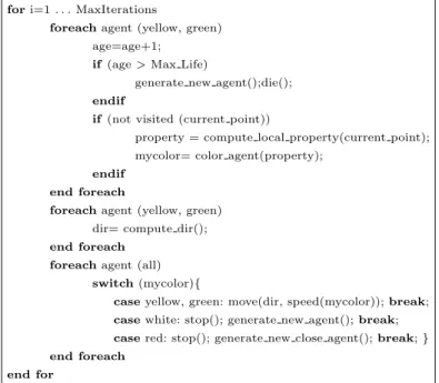
In figure 3.2, we summarized the pseudo code of the overall algorithm. Yellow and green agents will compute their direction, according to the rules previously described, and will move following this direction and with the speed corresponding to their color.
Agents will move towards the computed direction with a speed depending from their color: green agents more slowly than yellow agents since they will explore more interesting regions. An agent will speed up to leave an empty or uninteresting region whereas will slow down to investigate an interesting region more carefully.
The variable speed introduces an adaptive behavior in the algorithm. In fact, agents adapt their movement and change their behavior (speed) on the basis of their previous experience represented from the red and white agents. Red and white agents will stop signaling to the others respectively the inter-esting and desert regions. Note that, for any agent has become red or white, a new agent will be generated in order to maintain a constant number of agents
3.2 Flocking algorithm 23
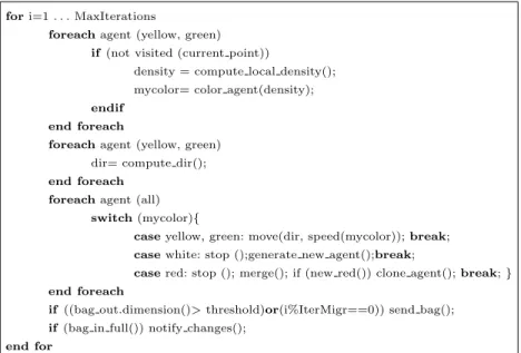
fori=1 . . . MaxIterations
foreachagent (yellow, green) age=age+1;
if(age > Max Life)
generate new agent();die(); endif
if(not visited (current point))
property = compute local property(current point); mycolor= color agent(property);
endif end foreach
foreachagent (yellow, green) dir= compute dir(); end foreach
foreachagent (all) switch(mycolor){
caseyellow, green: move(dir, speed(mycolor)); break; casewhite: stop(); generate new agent(); break; casered: stop(); generate new close agent(); break; } end foreach
end for
Fig. 3.2. The pseudo-code of the adaptive flocking algorithm.
exploring the data. In the first case (red), the new agent will be generated in a close random point, since the zone is considered interesting, while in the latter it will be generated in a random point over all the space. In case the agent falls in the same position of an older it will be regenerated using the same policy described above.
Note that the color of the agent is assigned on the basis of the desired property of the point in which it falls; the assignment is made on a scale going from white (property = 0) to red (property > threshold), passing for yellow and green, corresponding to intermediate values.
Yellow and green agents try to avoid the ’cage effect’ (see figure 3.3); in fact, some agents could remain trapped inside regions surrounded by red or white agents and would have no way to go out, wasting useful resources for the exploration. So, a limit was imposed on their life. When their age exceeded a determined value (M ax Lif e) they die and are regenerated in a new randomly chosen position of the space.
3.3 Clustering spatial data
In this section, we show how the stochastic search of the adaptive flocking described in the previous section can be used as a basis for implementing algorithms for clustering spatial data. Our approach has a number of nice properties. It can be easily implemented on parallel computers and is robust compared to the failure of individual agents. It can also be applied to per-form efficiently approximate clustering since the points, that are visited and analyzed by the agents, represent a significant (in ergodic sense) subset of the entire dataset. The subset reduces the size of the dataset while keeping the accuracy loss as small as possible.
In particular, we implemented SPARROW and SPARROW-SNN that re-spectively combine our flocking strategy with the DBSCAN heuristics for discovering clusters with differing sizes, shapes in noise data, and with the SNN heuristics in order to discover clusters with differing densities.
In the following, the DBSCAN algorithm and the SPARROW are de-scribed, then, SNN and SPARROW SNN are illustrated.
3.3.1 The DBSCAN algorithm
One of the most popular spatial clustering algorithms is DBSCAN, which is a density-based spatial clustering algorithm. A complete description of the algorithm and its theoretical basis is presented in the paper by Ester et al. [32]. In the following, we briefly present the main principles of DBSCAN. The algorithm is based on the idea that all points of a data set can be regrouped into two classes: clusters and noise. Clusters are defined as a set of dense connected regions with a given radius (Eps) and containing at least a minimum number (MinPts) of points. Data are regarded as noise if the number of points contained in a region falls below a specified threshold. The two parameters, Eps and MinPts, must be specified by the user and allow to control the density of the cluster that must be retrieved. The algorithm defines two different kinds of points in a clustering: core points and non-core points. A core point is a point with at least MinPts number of points contained in an Eps-neighborhood of the point. The non-core points in turn are either border points if are not core points but are density-reachable from another core point or noise points if they are not core points and are not density-reachable from other points. To find the clusters in a data set, DBSCAN starts from an arbitrary point and
3.3 Clustering spatial data 25
retrieves all points with the same density reachable from that point using Eps and MinPts as controlling parameters. A point p is density reachable from a point q, if the two points are connected by a chain of points such that each point has a minimal number of data points, including the next point in the chain, within a fixed radius. If the point is a core point, then the procedure yields a cluster. If the point is on the border, then DBSCAN goes on to the next point in the database and the point is assigned to the noise. DBSCAN builds clusters in sequence (that is, one at a time), in the order in which they are encountered during space traversal. The retrieval of the density of a cluster is performed by successive spatial queries. Such queries are supported efficiently by spatial access methods such as R*-trees.
3.3.2 SPARROW algorithm
SPARROW is a multi-agent adaptive algorithm able to discover clusters in parallel. It uses the modified version of standard flocking algorithm that incor-porates the capacity for learning that can find in many social insects. Flocking agents are transformed into hunters with a foraging behavior that allow them to explore the spatial data and to search for clusters.
SPARROW starts with a fixed number of agents that occupy a randomly generated position. Each agent moves around the spatial data testing the neighborhood of each location in order to verify if the point can be identified as a core (representative) point. Such a case, a temporary label is assigned to all the points of the neighborhood of the core point. The labels are updated concurrently as multiple clusters take shape. Contiguous points belonging to the same cluster take the label corresponding to the smallest label in the group of contiguous points.
The algorithm follows the same pseudo-code described in figure 5.1, but the compute property function is derived from DBSCAN and computes the local density of the points of clusters in the data belonging to the neighborhood of the current point, then the myColor procedure chooses the color and the speed of the agents with regard to this local density. The algorithm is based on the same parameters used in the DBSCAN algorithm: MinPts, the minimum number of points to form a cluster and Eps, the maximum distance that the agents can look at. In practice, the agent computes the local density (density) in a circular neighborhood (with a radius determined by its limited sight, i.e. Eps) and then it chooses the color in accordance to the following simple rules:
density > M inP ts ⇒mycolor= red (speed = 0)
M inP ts
4 < density ≤ M inP ts ⇒ mycolor= green (speed = 1)
0 < density ≤ M inP ts
4 ⇒mycolor= yellow (speed = 2)
In the running phase, the yellow and green agents will compute their di-rection, according to the rules previously described, and will move following this direction and with the speed corresponding to their color.
In addition, new red agents will run the merge procedure, which will merge the neighboring clusters. The merging phase considers two different cases: when we have never visited points in the circular neighborhood and when we have points belonging to different clusters. In the first case, the points will be labeled and will constitute a new cluster; in the second case, all the points will be merged into the same cluster, i.e. they will get the label of the cluster discovered first.
SPARROW suffers the same limitation as DBSCAN, i.e. it can not cope with clusters of different densities. A new algorithm SPARROW-SNN, intro-duced in the next subsection, is more general and overcomes these drawbacks. It can be used to discover clusters with differing sizes, shapes and densities in noise data.
3.3.3 The SNN algorithm
SNN is a clustering algorithm developed by Ert¨oz, Steinbach and Kumar [31] to discover clusters with differing sizes, shapes and densities in noise, high di-mensional data. The algorithm extends the nearest-neighbor non-hierarchical clustering technique by Jarvis-Patrick [54] redefining the similarity between pairs of points in terms of how many nearest neighbors the two points share. Using this new definition of similarity, the algorithm eliminates noise and outliers, identifies representative points, and then builds clusters around the representative points. These clusters do not contain all the points, but rather represent relatively uniform group of points. The SNN algorithm starts per-forming the Jarvis-Patrick scheme. In the Jarvis-Patrick algorithm a set of ob-jects is partitioned into clusters on the basis of the number of shared nearest-neighbors. The standard implementation is constituted by two phases. The first is a pre-processing stage that identifies the K nearest-neighbors of each object in the dataset. In the subsequent clustering stage, two objects i and j join the same cluster if:
• iis one of the Knearest − neighbors of j; • j is one of the Knearest − neighbors of i;
• iand j have at least Kmin of their Knearest − neighbours in common;
where K and Kmin are used-defined parameters. For each pair of points
i and j is defined a link with an associate weight. The strength of the link between i and j is defined as:
strength(i, j) =X(k + 1 − m)(k + 1 − n) where im= jn
In the equation above, k is the nearest neighbor list size, m and n are the positions of a shared nearest neighbor in i and j’s lists. At this point,
3.3 Clustering spatial data 27
clusters can be obtained by removing all edges with weights less than a user specified threshold and taking all the connected components as clusters. A major drawback of the Jarvis-Patrick algorithm is that, the threshold needs to be set high enough since two distinct set of points can be merged into same cluster even if there is only link across them. On the other hand, if a high threshold is applied, then a natural cluster will be split into many small clusters due to the variations in the similarity in the cluster.
SNN addresses these problems introducing the following steps.
1. For every node (data point) calculates the total strength (connectivity) of links coming out of the point;
2. Identify representative points by choosing the points that have high den-sity ( > core threshold);
3. Identify noise points by choosing the points that have low density ( < noise threshold) and remove them;
4. Remove all links between points that have weight smaller than a threshold (merge threshold);
5. Take connected components of points to form clusters, where every point in a cluster is either a representative point or is connected to a represen-tative point.
The number of clusters is not given to the algorithm as a parameter. Also note that not all the points are clustered.
3.3.4 SPARROW-SNN algorithm
Sparrow-SNN follows the pseucode of figure 3.2 and starts a fixed number of agents that will occupy a randomly generated position. From their initial position, each agent moves around the spatial data testing the neighborhood of each location in order to verify if the point can be identified as a representative (or core) point.
The compute property function represents the connectivity of the point as defined in SNN algorithm. In practice, when an agent falls on a data point A, not yet visited, it computes the connectivity, conn(A), of the point, i.e. computes the total number of strong links the points has, according to the rules of the SNN algorithm. Note that SPARROW-SNN computes for each data element the nearest-neighbor list using a similarity-threshold that reduces the number of data elements to take in consideration. The introduction of the similarity-threshold produces variable-length nearest-neighbor lists and therefore i and j must have at least Pmin of the shorter nearest-neighbor list
in common; where Pmin is a user-defined percentage.
Points having connectivity smaller than a fixed threshold (noise threshold ) are classified as noise and are considered for removal from clustering. Then a color is assigned to each agent, on the basis of the value of the connec-tivity computed in the visited point, using the following procedure (called color agent() in the pseudocode):
conn > core threshold ⇒mycolor= red (speed = 0) noise threshold < conn ≤ core threshold ⇒ mycolor= green (speed = 1)
0 < conn < noise threshold ⇒mycolor= yellow (speed = 2)
conn= 0 ⇒mycolor= white (speed = 0)
The colors assigned to the agents are: red, revealing representative points, green, border points, yellow, noise points, and white, indicating an obstacle (uninteresting region). After the coloration step, the green and yellow agents compute their movement observing the positions of all other agents that are at most at some fixed distance (dist max ) from their and applying the same rules as SPARROW. In any case, each new red agent (placed on a representative point) will run the merge procedure, as described in the Sparrow subsection, so that it will include, in the final cluster, the representative point discovered, and together to the points that share with it a significant (greater that Pmin) number of neighbors and that are not noise points. The merging phase con-siders two different cases: when we have visited none of these points in the neighborhood and when we have points belonging to different clusters. In the former, the same temporary label will be assigned and a a new cluster will be constituted; in the latter, all the points will be merged into the same cluster, i.e. they will get the label corresponding to the smallest label. So clusters will be built incrementally.
3.4 Experimental results
The following section shows the experimental results obtained for the two clustering algorithms. Both algorithms have been implemented using Swarm, a multi-agent software platform for the simulation of complex adaptive systems. In the Swarm system the basic unit of simulation is the swarm, a collection of agents executing a schedule of actions. Swarm provides object oriented libraries of reusable components for building models and analyzing, displaying, and controlling experiments on those models. More information about Swarm can be obtained from [86].
All the experiments were averaged over 30 tries. Where not differently specified, we run our algorithm using 50 agents and we set the visibility radius of the agents (dist max) to 6 and the minimum distance among the agents (dist min) to 2.
3.4.1 SPARROW results
We evaluated the accuracy of the solution supplied by SPARROW in com-parison with the one of DBSCAN and the performance of the search strategy of SPARROW in comparison with the standard flocking search strategy and with the linear randomized search. Furthermore, we studied the impact of the
3.4 Experimental results 29
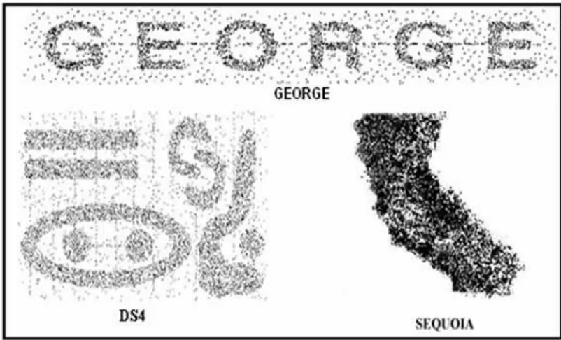
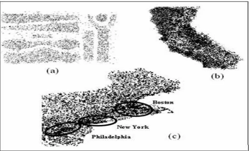
number of agents on foraging for clusters performance. Results are compared with the ones obtained using a publicly available version of DBSCAN. Our algorithm uses the same parameters as DBSCAN. Therefore, if we visited all the points of the dataset, we would obtain the same results. Then, in our experiments we consider as 100% the cluster points found by DBSCAN (note DBSCAN visit all the points). We want to verify how we come close to this percentage visiting only a portion of the entire dataset. For the experiments, we used two synthetic data sets and one real, shown in figure 3.4. The first data set, called GEORGE, consists of 5463 points. The second data set, called DS4, contains 8843 points. Each point of the two data sets has two attributes that define the x and y coordinates. Furthermore, both data sets have a con-siderable quantity of noise. The third called SEQUOIA is composed by 62556 names of landmarks (and their coordinates), and was extracted from the US Geological Survey’s Geographic Name Information System. We set eps to 9 for all the datasets and MinPts to 20 for George and DS4 and 40 for Sequoia.
Fig. 3.4. The three data sets used in our experiments.
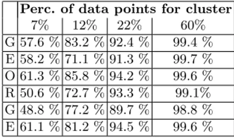
Although DBSCAN and SPARROW would produce the same results if we examined all points of the data set, our experiments showed that SPARROW can obtain, with an average accuracy about 93% on GEORGE dataset and about 78% on DS4, the same number of clusters with a slightly smaller per-centage of points for each cluster using only 22% of the spatial queries used by DBSCAN. The same results cannot be obtained by DBSCAN because of the different strategy of attribution of the points to the clusters. In fact, if we stopped DBSCAN before which it had performed the spatial queries on all the points, we should obtain a correct number of points for the clusters already individuated and probably a smaller number of points for the cluster that it was building, but obviously we will not discover all the clusters.
Perc. of data points for cluster 7% 12% 22% 60% G 57.6 % 83.2 % 92.4 % 99.4 % E 58.2 % 71.1 % 91.3 % 99.7 % O 61.3 % 85.8 % 94.2 % 99.6 % R 50.6 % 72.7 % 93.3 % 99.1% G 48.8 % 77.2 % 89.7 % 98.8 % E 61.1 % 81.2 % 94.5 % 99.6 %
Table 3.1. Number of clusters and number of points for clusters for GEORGE data set (percentage in comparison to the total point for cluster found by DBSCAN) when SPARROW analyzes 7%, 12%, 22% and 60% points.
Perc. of data points for cluster
7% 12% 22% 70% 1 51.16% 70.99% 78.86% 95.76 % 2 45.91% 64.74% 74.40% 95.45 % 3 40.68% 59.36% 81.95% 97.55 % 4 44.21% 60.66% 81.67% 98.05 % 5 54.65% 58.72% 71.54% 94.99 % 6 48.77% 59.91% 78.10% 97.76 % 7 54.29% 66.43% 79.18% 96.12 % 8 51.16% 70.99% 78.86% 96.33 % 9 45.91% 64.74% 74.40% 95.25 %
Table 3.2. Number of clusters and number of points for clusters for DS4 data set (percentage in comparison to the total point for cluster found by DBSCAN) when SPARROW analyzes 7%. 12%. 22% and 70% points.
Perc. of data points for cluster
7% 12% 22% 70%
S. Francisco 48.12% 66.22% 79.32% 98.88%
Sacramento 44.03% 61.11% 80.34% 97.56%
Los Angeles 51.21% 68.65% 81.92% 98.32%
Table 3.3. Number of clusters and number of points for clusters for Sequoia data set (percentage in comparison to the total point for cluster found by DBSCAN) when SPARROW analyzes 7%. 12%. 22% and 70% points.
3.4 Experimental results 31 0 100 200 300 400 500 0 50 100 150 200 250 300 350 400 450 500 Visited points Core Points Sparrow Flock Random
Fig. 3.5. Number of core points found for SPARROW, random and flock strategy vs. total number of visited points for the DS4 dataset.
0 100 200 300 400 500 0 50 100 150 200 250 300 350 400 450 500 Visited points Core Points Sparrow Flock Random
Fig. 3.6. Number of core points found for SPARROW, random and flock strategy vs. total number of visited points for the GEORGE dataset.
Table 1 and table 2 show, for the two data sets, the number of clusters and the percentage of points for each cluster found by DBSCAN and SPARROW. To verify the effectiveness of the search strategy, we have also compared SPARROW with the random-walk search (RWS) strategy of the Reynolds’ flock algorithm and with the linear randomized search (LRS) strategy.
Figure 3.5, 3.6 and 3.7 show the number of core points found for the three different strategies versus number of visited points respectively for the DS4, GEORGE and Sequoia data set. At the beginning, the random strategy, and also (to a minor extent) the flock, overcomes SPARROW, but, after 200-250 visited points SPARROW presents a superior behavior on both the search