Table of Contents
Acronyms and Abbreviations ... 3
1. Introduction ... 4
2. Summary of the critical review of the previous configuration ... 4
3. New reactor models ... 5
4. Characterization of the new core configuration ... 6
4.1. Investigation of ALFRED stability and dynamics ... 9
4.1.1. Stand-alone core analysis ... 9
4.1.2. Primary loop analysis ... 11
5. Steady state thermal-hydraulic verification ... 14
6. Conclusions ... 16
References ... 17
Appendix - Simulation tools for the assessment of the stability and the dynamics of the new ALFRED configuration ... 18
A.1. Model development ... 18
A.1.1. Neutronics ... 18
A.1.2. Thermal-hydraulics ... 18
A.1.3. Reactivity... 19
A.1.4. Primary loop ... 19
ADF – Axial Distribution Factor
ALFRED – Advance Lead Fast REactor European Demonstrator BoC – Beginnning of Cycle
BoL – Beginning of Life CR – Control Rod
DPA – Displacement Per Atom EoC – End of Cycle
FA – Fuel Assembly
FADF – Fuel Assembly Distribution Factor FPDF – Fuel Pin Distribution Factor GIF – Generation IV International Forum INN – Inner Fuel
LEADER – Lead-Cooled European Advance DEmonstration Reactor OUT – Outer Fuel
ALFRED – Advanced Lead Fast Reactor European Demonstrator – is the first nuclear reactor whose design has been entirely conceived and developed by an international community of researchers, taking inspiration from the ambitious concept expressed by the Generation IV International Forum (GIF) [1] for a new generation of nuclear energy systems more safe, clean, economical and proliferation resistant. Identified in the innovative technology of heavy liquid metals the more promising solution to reach the above mentioned objectives, ALFRED will have the double role of showing the idea’s validity, proving its technical feasibility, but also to quantitatively demonstrate the possibility of reaching degrees of safety, sustainability and economic competitiveness that will allow, to this new kind of reactors, meeting the population requests towards a sustainable and secure future [2-4].
In line with this vision, the present technical report is a continuation of the national and international studies and researches for the further development of the reactor design, with particular emphasis on the core design, in order to put to fruition the last two years of the Programmatic Agreement (Accordo di Programma) and finally establishing a new reference configuration for the ALFRED core. In particular, after the detailed analysis of the core configuration, as emerged from the LEADER project, in the last year we arrived at a possible arrangement in which all the revealed criticalities have been corrected [5]. The major aim of the activity of this year is the complete neutronic characterization, so as to retrieve enrichments and enrichment zoning which will allow to guarantee the operability of the reactor for the foreseen time span, respecting all the design constraints. The data obtained from this characterization will then be used to verify the assembly thermal-hydraulics and the pin thermo-mechanics, so as to cross-check the achievement of the aforementioned objectives. Since some modifications are expected also to impact on the reactivity coefficients, a model for the analysis of ALFRED dynamics will be developed, and applied to investigate the stability of the system.
2. Summary of the critical review of the previous configuration
In the last year of the Programmatic Agreement various critical points of the previous core configuration (Figure 1) were analyzed and appropriate solutions proposed, critically discussed and – where possible – tested estimating their impact on the design parameter they were directly acting upon. In a brief survey the proposed solutions were:
1) Enlargement of the wrapper inner key so to prevent overheating of the corner sub-channels. Combining this with the need to replace the original wrapper material, and having identified the 15-15Ti austenitic stainless steel as candidate, it was decided to reduce the thickness of the hexcan – taking profit of the superior mechanical performances of the latter with respect to T91 – in order to limit the impact on criticality.
2) A multifunctional shield with different elements in the different regions surrounding the multiplicative zone so to protect the inner vessel from excessive neutronic damage. The shield is composed of a reflecting region close to the core, and an absorbing region near the inner vessel.
3) In order to have more realistic simulations, in all the reactor models pure lead was substituted with one at a commercially available purity. The standard brand C1 was identified as the less expensive, still ensuring manageable polonium production.
data on the neutronic performances of the system.
These solutions and modeling choices, applied to the existing ALFRED configuration from the LEADER project, form the new reference configuration to be optimized and characterized.
Figure 1 - ALFRED core layout (one quarter), LEADER version.
3. New reactor models
Given the necessity of characterizing a new configuration so as to establish the reference core of ALFRED and given the material and geometrical modifications to be added to the model, it seems appropriate to update the ERANOS and MCNP input; moreover, considering that the previous input decks for the two codes were prepared by different organizations (specifically CEA for ERANOS 2.2 and ENEA for MCNP 6.1), some inconsistencies were present in the material properties or temperatures used. Moreover, the inputs were prepared under the LEADER and previous AdP projects thus not taking into account the new modifications object of the last year. In light of these considerations a coherent set of physical properties has been chosen – based on a literature review – and adopted for both codes; the temperatures of the various components of the reactor have been equalized and thermal dilatation has been calculated so as to be as much as possible realistic and consistent among the codes. A series of checks has also been performed in order to guarantee that the main masses and volumes were effectively equal between ERANOS 2.2 and MCNP 6.1, and now it can be stated that the main discrepancies in results are due to the different numerical approach of the codes and to the used cross section library sets; to prove this statement in Table 1 are reported the keff calculated by the codes along with the errors on the radial power map. It is worth mentioning that differences as low as 70 pcm (for criticality) and 1.3% (for power distribution) between ERANOS and MCNP results indicates the high coherence achieved in the development of the two models.
Code ERANOS 2.2 MCNP 6.1
Library JEFF3.1 JEFF3.1.2 ENDF/B-7.1b
keff 1.08307 1.08373±21pcm 1.07756±22pcm Max error on FA power at BoL (relative to MCNP-ENDF/B-7.1b) 1.32% 1.35% --
A note on the library set to be used in MCNP 6.1 must be made: the European reference library set is the JEFF-3.2 which however, in our tests, revealed problems in running coupled neutron and gamma calculations which are deemed essential in order to have the photonuclear contribution to the criticality and the power deposition in non fissile regions like the coolant, cladding etc. For this reason they cannot be used. In order not to use the previous (oldest) release JEFF-3.1.2 the choice has been directed towards the US ENDF/B-7.1b; this is justified because in runs with only neutron transport the JEFF-3.2 and ENDF/B-7.1b are very close to each other while the JEFF-3.1.2 predicts higher values for the keff as visible in Table 2.
Table 2 – MCNP 6.1 library confrontation for neutron only transport calculations.
Library JEFF-3.1.2 JEFF-3.2 ENDF/B-7.1b
keff 1.08367±21 pcm 1.07757±21 pcm 1.07767±20 pcm
Now that a common base for the codes has been settled, the core design can start; the results which will be show from now on are MCNP 6.1 results, but as stated, ERANOS 2.2 are very close and for the purpose of the neutronic design they can be effectively taken as equal.
4. Characterization of the new core configuration
The core design approach is an harmonization of thermal-hydraulic, mechanic and neutronic constraints in order to achieve certain goals, mainly related to safety, sustainability and economy. In the present study this approach will not be pursued since its very beginning because the fuel pin and assembly configuration are borrowed from the ALFRED core – LEADER version – plus the modifications previously discussed. The design will therefore be more oriented to the neutronic side in order to determine the new enrichments and enrichment zoning which will allow to guarantee the operability of the reactor for the foreseen time span, respecting all the constraints on the maximum cladding temperature and neutron damage on the reactor inner vessel internals (all constraints are borrowed from [3], but the main ones will be recalled in the present report).
One of the main limits to be respected is the 550°C on the cladding surface so to keep corrosion by liquid lead within acceptable levels; this must be respected throughout the whole core cycle in normal operation. The adopted neutronic design strategy is therefore to flatten as much as possible the clad temperature at pin level taking into account uncertainties from the
At EoC, coherently with the aim of maximizing fuel exploitation, the Control Rods (CR) are considered fully extracted, while at BoC they are inserted so as to compensate the reactivity excess required as reserve because of the burn-up swing. It then follows that the CRs are gradually withdrawn to compensate the fuel depletion and exactly at EoC they come in fully extracted position; this implies that on average the CRs are inserted halfway, or better, they are inserted so to give an anti-reactivity which is half the burn-up swing they are requested to compensate. Since the effect of the CRs is crucial at BoC, when it shifts the power distribution towards the core center and the upper portion of the active region (remembering that control rods in ALFRED are inserted from below), it is deemed necessary to take into account their effect. It must be said, however, that performing calculation with CRs movement is very difficult, sometimes lengthy if not even impossible (depending on the code). In the present work therefore a novel approach has been followed, which needs verification with direct calculation of the CR movements, enabling a realistic power map evaluation even without performing real CR movements during the burn-up simulations; the idea is to burn the core with the CR inserted halfway and evaluating the effect of their movement at BoC and EoC with calculations on a fresh core (BoL), with CRs fully inserted and fully extracted respectively. Through this it has been possible, by comparison with the half inserted calculation, to retrieve the correction factors to be applied to the Fuel Assemblies (FA), axial and pin-by-pin distributions factors. The factors calculated at BoL are applied at BoC and EoC assuming that the relative effect has been negligibly modified by the burnup; this is reasonable because the burnup swing is not very high and a relative effect such as this should be less sensitive than absolute effects, which are already small for the CRs in ALFRED. The calculated factor are reported in Table 3 where the two Axial Distribution Factors (ADF) correspond to the average value and the value for the end of the active length where the maximum cladding temperatures are located. Being the CRs inserted from below, it is important to account for their presence because they enhance power the top region of the core, where temperatures are indeed higher.
Table 3 – CRs insertion effect factors where FADF (FA Distribution Factor), ADF (Axial Distribution Factor) and FPDF (Fuel Pin Distribution Factor).
State BoC EoC
Region INN OUT INN OUT
FADF 1.093 0.994 0.932 1.006
ADF_average 1.003 1.020 0.992 0.974
ADF_end core 0.988 1.047 0.969 0.922
FPDF 1.011 1.024 1.009 0.979
The enrichment zoning has been left unchanged from the previous configuration, only their ratio and absolute value has been modified. In order to respect the constraint on the maximum linear power achievable (340÷350 W/cm) the active length has been slightly increased, passing from 60 to 65 cm, keeping fixed the number of pins in the core. This also permits to respect the maximum Burn-Up limit so as to not incur in excessive Pellet-Clad Mechanical
power in the central FA and the high gradient in the outer FA, the new enrichments have been found to be: 22.2 wt.% and 27.4 wt.% for the inner and outer zone respectively; the reactivity evolution during time is reported in Figure 2, where is visible the about unity keff at EoC and a burnup swing of 2440 pcm. The maximum FA power at BoC and EoC (already corrected for the CRs effect), along with the maximum linear power are reported in Table 4; it is seen that the constraint is actually respected even considering an increase of some 3-4% to account for the refueling effect not consider in the 1-batch approximation.
0 200 400 600 800 1000 1200 1400 1600 1800 2000 0,9 0,92 0,94 0,96 0,98 1 1,02 1,04 1,06 1,08 1,1 Days [d] K e ff
Figure 2 – keff evolution during burn-up.
Table 4 – Maximum power of the proposed configuration.
State BoC EoC
Region INN OUT INN OUT
Max FA power
[MW] 2.43 2.11 2.06 2.11
Max linear power
[W/cm] 332 326 299 298
The average DPA calculated for the cladding in the active region for the peak flux pin are around 83 which, when multiplied by the axial distribution factor, becomes 95 thus respecting the 100 design constraint. The peak vessel DPA after 60 years is around 2 equaling the design limit; if necessary, the value can be further reduced by extending the height of the absorber portion of the Absorber Dummy Element close to the vessel by some 30 cm above the active region.
It must be pointed out that the increased height will worsen the coolant density effect in the core region and due to the increased pressure drops (partially compensated by the larger
configuration [4] even in unprotected conditions, safety analysis are deemed necessary to confirm the performances of this option. Specifically referencing the increase of the coolant density effect, a dynamics analysis of ALFRED was performed to infer the stability of the system as a function of the associated reactivity coefficient.
4.1. Investigation of ALFRED stability and dynamics
Six different conditions have been considered to draw the poles of the system. In the first place, a stand-alone core configuration has been studied, in this case the inlet temperature is considered as a fixed input. In this condition, three major cases have been analyzed:
a) power level ranging between zero power and full nominal power at BoC; b) power level ranging between zero power and full nominal power at EoC;
c) parametric variation of the lead density reactivity coefficient on the entire power range at BoC.
In the second place, the simplified primary system configuration has been taken into account, and the effects of closing the loop on stability have been assessed. Similarly to the stand-alone core study, three cases have been considered:
a) power level ranging between zero power and full nominal power at BoC with SG at nominal conditions;
b) power level ranging between zero power and full nominal power at BoC with SG at ideal heat exchange conditions;
c) parametric variation of the lead density reactivity coefficient on the entire power range at BoC with SG at nominal conditions.
4.1.1. Stand-alone core analysis
A stand-alone core analysis has been carried out aimed at verifying the core system stability in nominal conditions at different power levels at BoC. In particular, the neutronics block has been treated as the open loop, whereas the thermal-hydraulics with its reactivity coefficients constitutes the feedback loop, as depicted in Figure 3.
Figure 3 – conceptual feedback scheme employed to describe the stand-alone core behavior.
A thirteenth order system has been obtained by implementing the equations associated to the model described in Appendix A. After simplification and linearization, a four roots system
All the system roots lay on the left hand side of the Gauss plane, confirming that the core is stable on the entire power range (Poles at -4700 rad/s and -2.5 rad/s are not shown and discussed in this analysis since they do not change their position significantly with varying power and lead coefficient, resulting in an almost constant contribution to the system behavior).
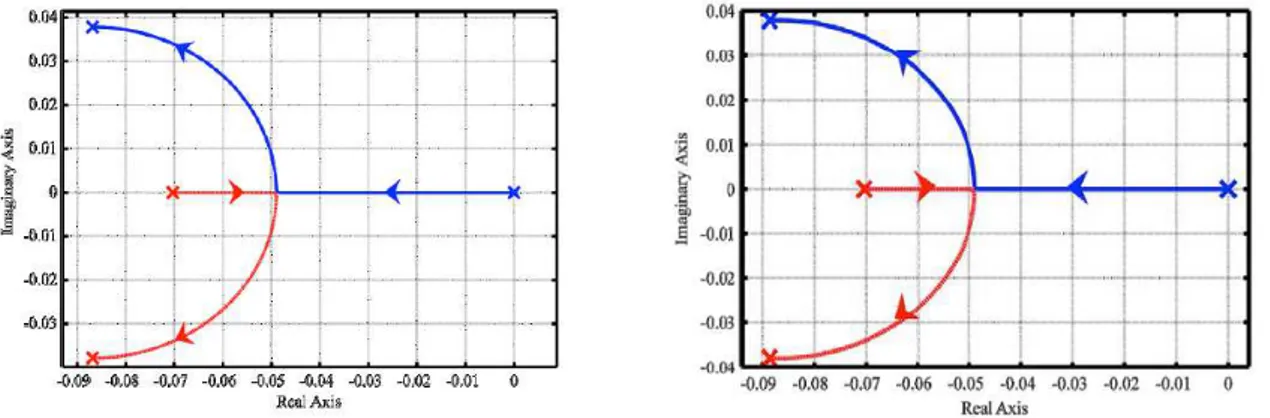
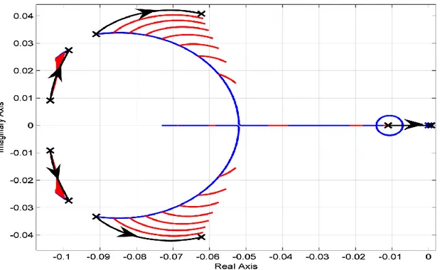
More in detail, the neutronics-related pole is located in the origin when the reactor is at zero power conditions, and moves to the left as the power rises, due to the increasing effect of the temperature-induced negative reactivity feedbacks. At a certain power level the dominant poles become complex conjugated, as shown in Figure 4, indicating that power fluctuations occur. In particular, the imaginary part of the poles increases along with the rising power level, meaning that the frequency of the oscillations increases too. Despite the rise of the imaginary part of the poles, the magnitude of the real negative part grants the damping of such oscillations. This phenomenon ensues from the fact that in the linearized model the gain of the thermal feedback is proportional to the power level; thus, for equal variations of reactivity, the oscillation frequency grows as the power increases.
An analogous behavior is found at EoC, whose root locus is shown on the right side of Figure 4: the core exhibits the same stability characteristics as at BoC, coherently with the very slight differences between the respective reactivity coefficients and kinetic parameters. As a consequence of such minor discrepancies, it can be concluded that the influence of the fuel burn-up is definitely negligible as far as the system stability is concerned.
Figure 4 – root locus detailed view for the stand-alone core as a function of power level at BoC (left) and EoC (right).
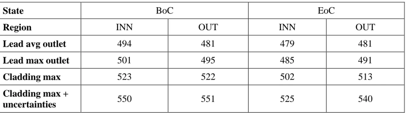
The core system stability has been investigated also when making the coolant density reactivity coefficient parametrically vary from its positive nominal value to large positive figures, so as to determine a critical threshold rendering the system unstable.
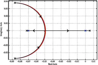
Figure 5 – root locus for the stand-alone core as a function of power level with the coolant density coefficient ranging from 0 to 12 pcm/K at BoC.
As shown in Figure 5, the blue track represents the poles trajectory as a function of power level (from 0 to 300 MWth) with the coolant density coefficient kept constant at its nominal value. The red lines represent the poles trajectories evaluated at discrete power levels (from 30 MWth to nominal power, with 10% steps) as a function of the coolant density coefficient varying from 0 to 12 pcm/K. In this latter case, for increasing values of the lead density coefficient, the roots move to the right, becoming first real and then also positive at a certain critical value around 12 pcm/K. Such a trend is not always the same since the critical value depends on the power level considered: actually, the system at nominal power becomes unstable for the lowest lead density coefficient (as described in Figure 5, black track). This trend is mainly due to the amplified feedback effects at higher power. In fact, if the action of a feedback is destabilizing (i.e., the corresponding reactivity coefficient is positive), its impact is first noticed at high power, where its magnitude is larger because more amplified. In addition, the (negative, that is stabilizing) Doppler effect is stronger at low power levels, and decreases along with the power level increase. Therefore, at low power levels there is a stronger counteraction by the Doppler effect, which counterbalances the lead density coefficient positive action. In other words, the core behavior is more sensitive to this design parameter variation at nominal power, and thus it may be concluded that, at low power levels, the system is more robust to uncertainties affecting its value. In any case, it has been seen that the system becomes unstable only for extremely high values of the coolant density coefficient, a clearly non-realistic condition.
Therefore, it can be stated that the system is inherently stable, and consequently safe, both at low power levels and in the case of positive coolant density reactivity coefficients.
4.1.2. Primary loop analysis
A stability analysis has been carried out also in a primary loop configuration in order to consider a more realistic situation in which the SG feedback action on the core dynamics is taken into account (Figure 6).
Figure 6 – conceptual feedback scheme employed to describe the primary loop behavior.
Equations representing the influence of the SG and the closure of the primary loop (see Appendix A) have been added to the previous set of equations, obtaining a total of sixteen equations. Also in this case, model simplification and linearization have reduced the dimension of the equation set: finally, a seven roots system has been considered.
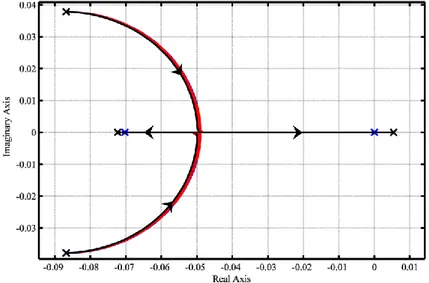
As Figure 7 illustrates, the system is still stable in nominal conditions at each power level, but compared to the previous case, additional complex conjugate poles appear in the plots: a new dynamics has been found on the right of the trajectories representing the stand-alone core; the new tracks are closer to the origin and complex conjugate for low power levels, suggesting that the dynamics they describe is slower and with damped oscillations In this case only one pole remains close to the origin also at high power levels, whereas in the stand-alone core analysis both the roots move to the left. As mentioned previously, when coupling the core with the SG the coolant core inlet temperature is no longer a fixed input, becoming instead a state variable depending on the power exchange conditions at the interface with the secondary side. This induces a feedback on the core behavior, whose neutronics is influenced by the reactivity effects led by temperature changes.
Figure 7 – root locus for the primary system as a function of power level at BoC, in nominal SG conditions (left) and ideal exchange conditions (right).
When the SG is set at nominal conditions, any power variation on the core side causes the core inlet temperature to change affecting the system reactivity (primarily due to the coolant temperature variation, with a consequent additional lead density and radial expansion feedback), differently than in the stand-alone core case, in which the inlet temperature is a fixed input. Such phenomena explain the system new oscillatory behavior at low power shown in Figure 7.
capabilities, the circle moves to the left and reduces its dimensions, meaning that oscillations progressively damp as the stand-alone core case is asymptotically approached (i.e. inlet temperature independent of the SG heat exchange capabilities). In both the above mentioned situations, the primary loop pole trajectories have been examined again as a function of the lead density coefficient variation (Figure 8).
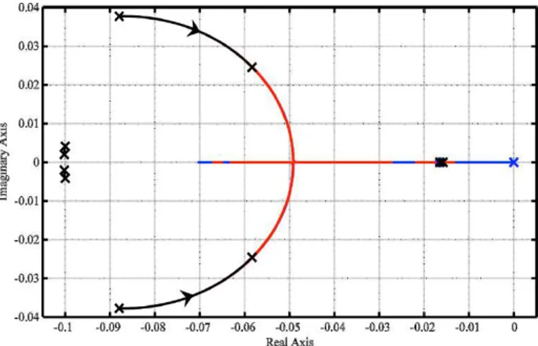
Figure 8 – root locus for the primary system as a function of power level with lead density coefficient ranging between 0 and 7 pcm/K at BoC, in nominal SG conditions.
As in the previous graphs, the blue track constitutes the roots trajectories when the power varies and the lead density coefficient is equal to its nominal value, whereas red tracks represent the poles motion induced by variations of the lead density coefficient from 0 to 7 pcm/K at each power level (the nominal power is depicted with black track).
By comparing Figure 8 with Figure 5,it can be inferred that the primary loop system behaves qualitatively as the stand-alone core one, but the instability threshold is reached earlier in the former case: for increasing values of the lead density coefficient the poles move to the right and become real positive when the coolant density coefficient is between 6 and 7 pcm/K, evidencing a kind of “destabilizing” action by the SG.
Figure 9 – root locus for the primary system as a function of power level with lead density coefficient ranging between 0 and 7 pcm/K at BoC, in ideal perfect exchange conditions.
conditions are to the ideal ones, the higher is the margin of stability of the reactor system, since the core is less and less influenced by the secondary side dynamics. Indeed, when considering an ideal SG (Figure 9), the poles never reach a positive real part for the considered range of the lead density coefficient, implying that greater values of the reactivity coefficient are needed for the system to become unstable, likewise in the only core case (Figure 5).
Anyway, even when considering the closed system configuration with nominal SG conditions, the reactor becomes unstable only for very high values of the lead density coefficient, which are still non-realistic. Therefore, it can be definitely concluded that the overall system is indeed inherently stable, and consequently safe.
5. Steady state thermal-hydraulic verification
In order to check the consistency of the adopted design methodology and to ensure that the temperature constraints are effectively met under steady state conditions, a detailed analysis at FA level is necessary. The numerical method selected for this purpose is the sub-channel one by means of the ANTEO+ code [6]. In order to have simulations as realistic as possible, only the portion of the power reported in Table 4 which is actually produced in the fuel is considered, i.e. approximately 93/94%; the remaining portion is used to calculate the temperature gain of the lead in the following way: a temperature increase is calculated which is then added to the nominal inlet temperature (400°C) so to preserve the heat balance of lead and the temperature difference between coolant and clad. All this is necessary because in ANTEO+ all the power is generated in the fuel. The nominal flow rate has been deduced by a new gagging scheme coherent with the new power distribution; for each FA the flow rate giving a coolant bulk temperature increase of 80°C has been calculated for both BoC and EoC. The average of the two configurations has been taken and plotted in order to easily identify the FAs with similar flow rates; from this, four cooling groups have been defined, which are characterized by the average of the flow rates of each FA composing the group. Since the power is more peaked in the core center, in the new gagging scheme the flow has been increased for the central FAs with respect to the LEADER version.
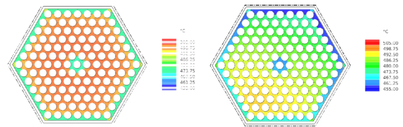
Figure 10 – BoC lead temperature distribution at core outlet in the hottest FAs of the INN (left) and OUT (right) core regions.
Figure 11 – EoC lead temperature distribution at core outlet in the hottest FAs of the INN (left) and OUT (right) core regions.
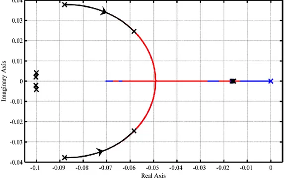
Results of the verification analysis are reported in Figures 10-11 and Table 5 where the effect of uncertainties coming from physical properties, geometry, power distributions, measurements and control systems dead bands are taken into account with a semi-statistical vertical approach in the evaluation of the maximum cladding temperature. In particular, the 3σ uncertainties for the bulk lead temperature gain is 20% while for the clad-bulk is around 38%.
Table 5 – Outlet lead and cladding temperatures.
State BoC EoC
Region INN OUT INN OUT
Lead avg outlet 494 481 479 481
Lead max outlet 501 495 485 491
Cladding max 523 522 502 513
Cladding max +
uncertainties 550 551 525 540
As can be seen, all the imposed temperature constraints are basically respected even when uncertainties are taken into account, thus proving the effectiveness of the proposed core configuration in steady state situations.
Closing the path delineated in the last two years of the Programmatic Agreement, the core of ALFRED as emerged from the LEADER project has been critically revised in a large spectrum of aspects in order to arrive to a core configuration mature enough to be taken as reference for the conceptual design stage. In this work the neutronic characterization of the new ALFRED core has been presented with the aim of flattening as much as possible the maximum clad temperature at pin level taking into account both CR movements during irradiation and uncertainties. DPA calculations for the critical components inside the vessel have also been reported, successfully complying with the design constraints.
In order to check the consistency of the adopted design methodology and to ensure that the temperature constraints are effectively met under steady state conditions, a detailed analysis at FA level has been performed. The thermal-hydraulic verification has revealed the robustness of the proposed configuration in nominal conditions where all the temperature-related constraints have been respected.
Concluding, the ALFRED core configuration here described is proposed as new reference for future analysis, remembering that further work will include the calculation of all the reactivity coefficients followed by a detailed safety analysis to test the degree of forgiveness to be reckoned to the plant design as a whole.
[1] U.S. Department Of Energy Nuclear Energy Research Advisory Committee and Generation IV International Forum. A Technology Roadmap for Generation IV Nuclear Energy Systems. Technical Report GIF(2002), http://www.gen-4.org/Technology/roadmap.htm.
[2] G. Grasso et al. A core design approach aimed at the sustainability and intrinsic Safety of the European Lead-cooled Fast Reactor. In Proceedings of Fast Reactors and Related Fuel Cycles: Safe Technologies and Sustainable Scenarios (FR13), Paris, France, March 4-7, 2013.
[3] G. Grasso et al. Demonstrating the effectiveness of the European LFR concept: the ALFRED core design. In Proceedings of Fast Reactors and Related Fuel Cycles: Safe Technologies and Sustainable Scenarios (FR13), Paris, France, March 4-7, 2013.
[4] E. Bubelis et al. LFR safety approach and main ELFR safety analysis results. In Proceedings of Fast Reactors and Related Fuel Cycles: Safe Technologies and Sustainable Scenarios (FR13), Paris, France, March 4-7, 2013.
[5] G. Grasso, F. Lodi et al. Ottimizzazione del progetto di nocciolo di ALFRED. Ricerca di Sistema Elettrico, Technical Report ADPFISS-LP2-050, 2014.
[6] F. Lodi, G. Grasso, D. Mattioli, M. Sumini. ANTEO+: a subchannel code for thermal-hydraulic analysis of liquid metal cooled systems. NED-D-15-00315 Under Review, Nuclear Engineering and Design, 2015.
In this section, the simulation tool devoted to the stability analysis is described along with the procedure adopted to perform the linear stability analysis. The stability analysis has been carried out both for the stand-alone core and the coupled primary loop configuration. Moreover, the impact of the coolant density reactivity coefficient on stability has been evaluated by considering both configurations. Such a study has been meant to provide the reactor designer with quantitative feedbacks concerning this key parameter from a safety-related perspective. Indeed, being the coefficient tightly dependent on the core arrangement, in terms of both geometrical and material buckling, it is expected that significant differences may occur between the demonstrator and the industrial scale LFR, with consequent impact on dynamics. Therefore, the system stability has been investigated against the lead density reactivity coefficient value in order to assess a theoretical threshold making the reactor unstable, so that the core designer can adopt suitable provisions to ensure the reactor operates under stable conditions in any situation beyond nominal. Finally, in order to evaluate the dynamic characteristics of the system as a function of the core lifetime, calculations have been carried out at BoC and EoC, so as to assess also the effects of the fuel burn-up.
A.1. Model development
An analytical zero-dimensional model accounting of all the main feedbacks following a reactivity change in the core has been implemented incorporating a point-wise kinetics description for neutronics coupled with a single-channel, average-temperature heat transfer treatment for thermal-hydraulics.
A.1.1. Neutronics
Point-wise kinetics with one neutron energy group and eight delayed neutron precursor groups has been employed for the core neutronics model, in which the total power is considered as generated only by fission events, while the contribution of decay heat being neglected.
In the present model scheme, a further simplified version has been adopted, in which all the precursor groups have been collapsed into a unique one, by means of an abundance-weighted average decay constant (Hetrick, 1971).
The main drawback of this model is the impossibility to describe a spatial dependence of the neutron population behavior, since the relationship between the latter and thermal power prevents from mapping the thermal power density within the core.
A.1.2. Thermal-hydraulics
A zero-dimensional approach has been adopted to treat also the system thermal-hydraulics. Some simplifying hypotheses have been assumed and a single-node heat transfer model has been implemented by accounting of three distinct temperature regions – corresponding to fuel, coolant and cladding –, enabling the reactivity feedback to include all the major contributions as well as the margin against technological limits to be monitored. In line with
Furthermore, a separate, multi-zone pin model accounting of the temperature distribution from the fuel centerline to the coolant bulk has been employed to calculate global heat transfer coefficients, by assuming physical properties and thermal resistances of fuel, gap and cladding to be constant with temperature and time, and neglecting thermal diffusion in the axial direction within the fuel pin.
As far as the dynamic variation of the fuel internal and external temperatures is concerned, the heat transfer process has been achieved by taking an energy balance over two fuel zones, where the fission power generated within the fuel is taken from the neutron kinetics equations and is treated as an input for the heat transfer dynamic model.
For the gradient of the cladding surface temperature, an energy balance has been applied. Finally, for the energy balance equation within the coolant, the respective temperature at the end of the channel has been assumed as a state variable; being the coolant inlet temperature a fixed input, an energy balance has been written as well.
Calculations of material properties have been performed in correspondence with the average nominal steady-state temperatures and the parameters obtained have been kept constant for the stability analyses.
A.1.3. Reactivity
Consistently with the lumped parameter modeling employed, the reactivity feedback function has been expressed as a function of the average values of fuel and coolant temperatures. Moreover, externally introduced reactivity has been simulated by the coefficient associated with the insertion length of a representative control rod, which has been handled as a simple input parameter.
As far as the Doppler coefficient determination is concerned, an effective average fuel temperature that accounts for resonances broadening, has been calculated at each power level (ranging from 10 % to 100 % nominal) as indicated by Kozlowski and Downar (2007) as a function of the internal and external surface fuel temperatures. The magnitude of the actual reactivity variation from a generic fuel temperature distribution to another specific one around the steady-state value has been evaluated based on (Waltar et al., 2012), allowing to define the Doppler coefficient at each power level.
In this work, a linear relation for core expansions (axial and radial) and coolant density reactivity effects has been adopted, leading to an expression incorporating constant coefficients and where stationary average temperatures have been calculated in correspondence with each power level considered.
A.1.4. Primary loop
In order to evaluate the system stability when considering also the entire primary loop configuration, a simplified treatment has been adopted to describe the coolant flowing towards the Steam Generator (SG) after being heated in the core, being cooled while passing through the SG and coming back to the core through the cold leg and coolant pool.
taking its energy balance. More specifically, the SG has been modeled so that in nominal conditions the difference between core outlet and inlet coolant temperature is equal to the nominal value (80°C), whereas in ideal heat exchange conditions the cold leg temperature is kept constant and equal to the saturation temperature of the secondary loop, which depends only on SG pressure, regardless of the power produced in the core. In such a system, the coolant core inlet temperature is no longer an input variable, but a state variable determined by the power exchange conditions on the SG side. On the other hand, when “ideal heat exchange conditions” are considered, the SG is assumed to be able to remove any power produced in the core, thus keeping the lead temperature in the cold leg always close to the nominal value (i.e. 400°C).
A.2. Method
The analytical zero-dimensional model introduced above has been simplified and linearized so as to enable the use of the linear analysis theory to verify the reactor stability on the entire power range and in different conditions through calculation of the system eigenvalues.
According to the linear analysis theory, the dynamic behavior of a linear system depends on the eigenvalues of the state matrix. This principle is still applicable to a linearization of a non-linear system around a certain steady state condition (Lyapunov, 1966). Thus, such linearization has been performed on the set of equations associated to the phenomena and assumptions previously described, and it has been possible to express the model in terms of the following matrix system:
+ = + = Du Cx y Bu Ax x&
where x is the vector of the state variables, u the input vector, y the output vector, A the state matrix, B and C the corresponding matrices, and D is an empty matrix since there is no feedthrough between input and output variables. This allows to focus on the matrix A and its eigenvalues, which represent the carriers of the dynamic response of the system; the latter, alternatively defined as poles or roots of the system, have been calculated through proper MATLAB® (The MathWorks Inc., 2015) scripts.
The position of the poles and their trajectories across the Gauss plane describe the dynamic behavior of the reactor: in order for the system to be stable, it is necessary that all poles remain in the left hand side of the plane in any working condition and following any perturbation of the nominal parameters, as discussed in the following case studies (Lyapunov, 1966).
DIPARTIMENTO DI ENERGIA, Sezione INGEGNERIA NUCLEARE-CeSNEF
Simulation tools for the assessment of the stability and
the dynamics of the new ALFRED configuration
Antonio Cammi, Stefano Lorenzi
CERSE-POLIMI RL 1602/2015
Milano, Settembre 2015
Lavoro svolto in esecuzione dell’Attività LP2.A.1_C
AdP MSE-ENEA sulla Ricerca di Sistema Elettrico - Piano Annuale di Realizzazione 2014 Progetto B.3.1 "Sviluppo competenze scientifiche nel campo della sicurezza nucleare e
LP2.A.3_A 1 CERSE-POLIMI RL 1602/2015 (this page is intentionally left blank)
LP2.A.3_A 2 CERSE-POLIMI RL 1602/2015
Index
INTRODUCTION __________________________________________________________ 4 LIST OF SYMBOLS ________________________________________________________ 6 LIST OF FIGURES _______________________________________________________ 10 LIST OF TABLES ________________________________________________________ 14 1. STABILITY ANALYSIS TOOL ___________________________________________ 16 1.1MODEL DEVELOPMENT ________________________________________________ 16 1.2METHOD ___________________________________________________________ 21 1.3RESULTS ___________________________________________________________ 22 2. OBJECT-ORIENTED SIMULATOR_______________________________________ 30 2.1.OBJECT-ORIENTED APPROACH __________________________________________ 31 2.2.MODEL DEVELOPMENT ________________________________________________ 33 2.3FREE DYNAMICS SIMULATIONS __________________________________________ 46 2.4STABILITY ANALYSIS VERIFICATION ______________________________________ 54 REFERENCES ___________________________________________________________ 60 CONCLUSIONS __________________________________________________________ 62 APPENDIX A: ALFRED REACTOR DESCRIPTION __________________________ 64LP2.A.3_A 3 CERSE-POLIMI RL 1602/2015 (this page is intentionally left blank)
LP2.A.3_A 4 CERSE-POLIMI RL 1602/2015
Introduction
The Lead-cooled Fast Reactor (LFR) is under development worldwide as a very promising fast neutron system to be operated in a closed fuel cycle. As recognized by the European Sustainable Nuclear Energy Technology Platform (SNETP), the LFR development requires as a fundamental intermediate step the realization of a demonstration plant intended to prove the viability of the technology as well as the overall system behavior. Advanced reactor concepts cooled by Heavy Liquid Metals Coolants (HLMCs) offer a great potential for plant simplifications and higher operating efficiencies compared to other coolants, introducing however additional safety concerns and design challenges.
This work is grafted in the research activity of the Nuclear Reactor Group of the Politecnico di Milano on LFRs In the framework of the “characterization of the new ALFRED core configuration”, the POLIMI effort has been spent in order to provide the designers with important feedbacks on the stability and dynamics of the reactor system. To this purpose, the simulation tools should be expressly meant for this phase of the new characterization of ALFRED reactor design, in which all the system specifications are reconsidered and thus are subject to modifications. Accordingly, the report is aimed at presenting two very flexible, straightforward and fast-running (i.e., without significant computational burden and implementation-related effort) simulation tools.
The first simulation tool is directed to the stability analysis and consist of an analytical lumped-parameter model incorporating a point-wise kinetics description for neutronics coupled with a single-channel, average temperature heat transfer treatment for thermal-hydraulics. The simplicity of the modelling, implemented in MATLAB, relies upon the fact that the model has to be linearize in order to study the stability.
The second simulation tool is devoted to study the dynamics and verifying the outcomes of the stability analysis with a higher level of modelling accuracy. To this end, an object-oriented model is proposed to be both accurate and fast-running. The overall plant simulator, incorporating also the BoP, consists of the following essential parts: core, steam generator,
LP2.A.3_A 5 CERSE-POLIMI RL 1602/2015 primary and secondary pumps, cold and hot legs, cold pool, turbine, and condenser. The model is developed with the Modelica language in the Dymola environment.
For the time being, the investigations are focused on the final configuration of the LEADER project, which can be considered the starting point of the new characterization. Nevertheless, in the further activities, the simulation tools developed in this report are foreseen to be adopted to study and finalize the new configuration.
LP2.A.3_A 6 CERSE-POLIMI RL 1602/2015
List of symbols
Latin Symbols
A single channel coolant flow area [m2] ACR coefficient for the calibration of CRs [pcm]
ASR coefficient for the calibration of SRs [pcm]
Av flow area [m2]
BCR coefficient for the calibration of CRs [ m-1]
Bo boiling number [-]
c average specific heat capacity [J kg-1 K-1] CCR coefficient for the calibration of CRs [-]
ci density of the ith precursor group [cm-3]
Cf Fanning friction coefficient [-]
Co Convection number [-] d density [kg m-3]
DCR coefficient for calibration of CRs [pcm]
f friction factor [-] FFl fluid-surface parameter
FrLO Froude number with all flow as liquid
g gravitational acceleration [m s-2] h specific enthalpy [J kg-1]
hcl Cladding-coolant global heat transfer coefficient [W K-1]
hCR height of control rods [m]
hLO single-phase heat transfer coefficient with all flow as liquid [W m-2 K-1]
hSR height of safety rods [m]
hTP two phase heat transfer coefficient [W m-2 K-1]
iLG latent heat of vaporization [J kg-1]
k thermal conductivity [W m-1 K-1] K pressure coefficient [m-2 s-2] KD Doppler constant [pcm]
LP2.A.3_A 7 CERSE-POLIMI RL 1602/2015 Keq Equivalent exchange unit [W K-1]
kv turbine admission valve coefficient [m s]
kf Fuel thermal conductivity [W m-1 K-1]
kfc Fuel-gap-cladding global heat transfer coefficient [W K-1]
LSR total length of SRs [m]
M Mass [kg]
n neutron density [cm-3] N number of axial nodes [-] Nu Nusselt number [-]
P Reactor thermal power [MW] p pressure [Pa]
Pe Peclet number [-] q neutron source [cm-3 s-1] q'' heat flux [W m-2]
q''' thermal power density [W m-3] r radial coordinate [m]
R radius [m] t time [s]
T average temperature [K] u fluid velocity [m s-1] w mass flow rate [kg s-1] x axial coordinate [m] xc critical ratio [-]
xv vapour quality [-]
xSR height of SRs at full power [m]
z elevation [m] Greek Symbols
αCR radial cladding expansion reactivity coefficient [pcm K-1]
LP2.A.3_A 8 CERSE-POLIMI RL 1602/2015 αD Doppler reactivity feedback coefficient [pcm K-1]
αDia diagrid expansion reactivity coefficient [pcm K-1]
αFZ axial fuel expansion reactivity coefficient [pcm K-1]
αH Control rod reactivity feedback coefficient [pcm m-1]
αL coolant density reactivity coefficient [pcm K-1]
αPad pad effect reactivity coefficient [pcm K-1]
αR Radial expansion reactivity feedback coefficient [pcm K-1]
αZ Axial expansion reactivity feedback coefficient [pcm K-1]
αWR radial wrapper expansion reactivity coefficient [pcm K-1]
αWZ axial wrapper expansion reactivity coefficient [pcm K-1]
β DNP total fraction [pcm]
βi DNP fraction of the ith precursor group [pcm]
Λ neutron generation time [s] c coefficient of discharge [-]
λi decay constant of the ith precursor [s-1]
ρ reactivity [pcm]
ρ0 reactivity margin stored in the core [pcm]
τHL Hot leg coolant circulation time constant [s]
τSG Steam generator coolant circulation time constant [s]
τCL Cold leg and pool coolant circulation time constant [s]
heat flux entering the tube (lateral surface) [W m-2] tube perimeter [m]
Superscripts D Doppler eff effective
1,3 fuel internal and external regions Subscripts
0 steady-state c cladding
LP2.A.3_A 9 CERSE-POLIMI RL 1602/2015 CBD convective boiling dominant
down downstream ext external f fuel g gap i inner in inlet int internal l lead coolant L liquid
NBD nucleate boiling dominant o outer out outlet sat saturation sg steam generator up upstream V vapour
LP2.A.3_A 10 CERSE-POLIMI RL 1602/2015
List of figures
Figure 1. Conceptual feedback scheme employed to describe the stand-alone core behavior. .... 23 Figure 2. Root locus detailed view for the stand-alone core as a function of power level at BoC (left) and EoC (right). ... 24 Figure 3. Root locus for the stand-alone core as a function of power level with 0 < L < 12 pcm
K−1 at BoC. ... 25 Figure 4. Conceptual feedback scheme employed to describe the primary loop behavior. ... 25 Figure 5. Root locus for the primary system as a function of power level at BoC, nominal SG conditions (left) and ideal exchange conditions (right). ... 26 Figure 6. Root locus for the primary system as a function of power level with 0 < L < 7 pcm K−1
at BoC, nominal SG conditions. ... 27 Figure 7. Root locus for the primary system as a function of power level with 0 < L < 7 pcm
K−1 at BoC, ideal perfect exchange conditions. ... 28 Figure 8. ALFRED object-oriented model. ... 33 Figure 9. ALFRED core object-oriented model. ... 34 Figure 10. Fuel pin radial scheme for heat transfer modelling. ... 36 Figure 11. Calibration curve of control rods and safety rods. ... 36 Figure 12. Fuel assembly geometry (lengths are expressed in mm). ... 39 Figure 13. Detailed view of ALFRED core: representation of coolant channels. ... 40 Figure 14. ALFRED SG object-oriented model. ... 42 Figure 15. ALFRED reactor secondary side. ... 45
LP2.A.3_A 11 CERSE-POLIMI RL 1602/2015 Figure 16. Variables evolution after a feedwater mass flow rate reduction: (a) SG pressure variation; (b) lead SG outlet temperature variation; (c) average lead temperature variation; (d) net reactivity variation; (e) core thermal power variation; (f) average fuel temperature variation; (g) core outlet temperature variation; (h) steam temperature variation. ... 48 Figure 17. Variables evolution after a variation of the turbine admission valve coefficient: (a) SG pressure variation; (b) lead SG outlet temperature variation; (c) net reactivity variation; (d) core thermal power variation; (e) core outlet temperature; (f) steam temperature variation. ... 51 Figure 18. Variables evolution after a step reactivity variation: (a) net reactivity variation; (b) core thermal power variation; (c) core outlet temperature variation; (d) steam temperature variation; (e) SG pressure variation; (f) lead SG outlet temperature variation; (g) average fuel temperature variation; (h) average lead temperature variation. ... 53 Figure 19. Variables evolution after a step reactivity variation, stand alone core with αL = 9
pcm/K: (a) core thermal power variation; (b) net reactivity variation; (c) average fuel temperature variation; (d) average lead temperature variation. ... 55 Figure 20. Variables evolution after a step reactivity variation, stand alone core with αL = 13
pcm/K: (a) core thermal power variation; (b) net reactivity variation; (c) average fuel temperature variation; (d) average lead temperature variation. ... 55 Figure 21. Variables evolution after a step reactivity variation, stand alone core with αL = 13
pcm/K at reduced power level: (a) core thermal power variation; (b) net reactivity variation; (c) average fuel temperature variation; (d) average lead temperature variation. ... 56 Figure 22. Variables evolution after a step reactivity variation, primary loop with αL = 2 pcm/K:
(a) core thermal power variation; (b) net reactivity variation; (c) average fuel temperature variation; (d) average lead temperature variation. ... 57 Figure 23. Variables evolution after a step reactivity variation, primary loop with αL = 7 pcm/K:
(a) core thermal power variation; (b) net reactivity variation; (c) average fuel temperature variation; (d) average lead temperature variation. ... 58
LP2.A.3_A 12 CERSE-POLIMI RL 1602/2015 Figure 24. Variables evolution after a step reactivity variation, primary loop with αL = 7 pcm/K
at reduced power level: (a) core thermal power variation; (b) net reactivity variation; (c) average fuel temperature variation; (d) average lead temperature variation. ... 59 Figure 25. ALFRED nuclear power plant layout ... 64 Figure 26. ALFRED core configuration. ... 66 Figure 27. ALFRED bayonet tube SG configuration ... 67
LP2.A.3_A 13 CERSE-POLIMI RL 1602/2015 (this page is intentionally left blank)
LP2.A.3_A 14 CERSE-POLIMI RL 1602/2015
List of tables
Table 1. Main features and differences between causal and acausal approach. ... 32 Table 2. ALFRED core parameters. ... 65 Table 3. ALFRED SG major nominal parameters. ... 67
LP2.A.3_A 15 CERSE-POLIMI RL 1602/2015 (this page is intentionally left blank)
LP2.A.3_A 16 CERSE-POLIMI RL 1602/2015
1. Stability analysis tool
In this section, the simulation tool devoted to the stability analysis is described along with the procedure adopted to perform the linear stability analysis. The stability analysis has been carried out both for the stand-alone core and the coupled primary loop configuration. Moreover, the impact of the coolant density reactivity coefficient on stability has been evaluated by considering both configurations. Such a study has been meant to provide the reactor designer with quantitative feedbacks concerning this key parameter from a safety-related perspective. Indeed, being the coefficient tightly dependent on the core arrangement, in terms of both geometrical and material buckling, it is expected that significant differences may occur between the demonstrator and the industrial scale LFR, with consequent impact on dynamics. Therefore, the system stability has been investigated against the lead density reactivity coefficient value in order to assess a theoretical threshold making the reactor unstable, so that the core designer can adopt suitable provisions to ensure the reactor operates under stable conditions in any situation beyond nominal. Finally, in order to evaluate the dynamic characteristics of the system as a function of the core lifetime, calculations have been carried out at BoC and EoC, so as to assess also the effects of the fuel burn-up.
1.1 Model development
An analytical zero-dimensional model accounting of all the main feedbacks following a reactivity change in the core has been implemented incorporating a point-wise kinetics description for neutronics coupled with a single-channel, average-temperature heat transfer treatment for thermal-hydraulics.
1.1.1 Neutronics
Point-wise kinetics with one neutron energy group and eight delayed neutron precursor groups has been employed for the core neutronics model, in which the total power is considered as generated only by fission events, while the contribution of decay heat being neglected:
dn(t) dt = ρ(t)−β Λ n(t) + ∑ λici(t) 8 i=1 (1)
LP2.A.3_A 17 CERSE-POLIMI RL 1602/2015
dci(t) dt =
βi
Λn(t) − λici(t) (2)
Equations (1) and (2) represent nine Ordinary Differential Equations (ODEs): Eq. (1) is a nonlinear equation for neutron density and Eqs. (2) are linear equations for precursor densities. In the present model scheme, a further simplified version has been adopted, in which all the precursor groups have been collapsed into a unique one, by means of an abundance-weighted average decay constant (Hetrick, 1971):
1 𝜆 = 1 𝛽∑ 𝛽𝑖 𝜆𝑖 8 𝑖=1 (3)
The main drawback of this model is the impossibility to describe a spatial dependence of the neutron population behavior, since the relationship between the latter and thermal power prevents from mapping the thermal power density within the core.
1.1.2 Thermal-hydraulics
A zero-dimensional approach has been adopted to treat also the system thermal-hydraulics. Some simplifying hypotheses have been assumed and a single-node heat transfer model has been implemented by accounting of three distinct temperature regions – corresponding to fuel, coolant and cladding –, enabling the reactivity feedback to include all the major contributions as well as the margin against technological limits to be monitored. In line with the point model concept, the latter temperatures have been assumed to be functions separable in space and time.
Furthermore, a separate, multi-zone pin model accounting of the temperature distribution from the fuel centerline to the coolant bulk has been employed to calculate global heat transfer coefficients, by assuming physical properties and thermal resistances of fuel, gap and cladding to be constant with temperature and time, and neglecting thermal diffusion in the axial direction within the fuel pin.
As far as the dynamic variation of the fuel internal and external temperatures is concerned, the heat transfer process has been achieved by taking an energy balance over two fuel zones:
Mf,int𝑐fdTf int(t) dt = Pint(t) − kf(Tf int(t) − T fext(t)) (4) Mf,ext𝑐fdTf ext(t) dt = Pext(t) + kf(Tf int(t) − T fext(t)) − kfc(Tfext(t) − Tc(t)) (5)
LP2.A.3_A 18 CERSE-POLIMI RL 1602/2015 where the fission power generated within the fuel is taken from the neutron kinetics equations according to Eq. (6), in which the subscript 0 indicates steady-state values, and is treated as an input for the heat transfer dynamic model:
n(t) n0 =
P(t)
P0 (6)
For the gradient of the cladding surface temperature, the following energy balance has been applied:
Mc𝑐cdTdtc(t)= kfc(Tfext(t) − Tc(t)) − hcl(Tc(t) − Tl,out(t)) (7)
Finally, for the energy balance equation within the coolant, the respective temperature at the end of the channel has been assumed as a state variable; being the coolant inlet temperature a fixed input, the energy balance has been written as:
MlcldTl,outdt (t)= hcl(Tc(t) − Tl ,out(t)) − wcl(Tl,out(t) − Tl,in(t)) (8)
Calculations of material properties have been performed in correspondence with the average nominal steady-state temperatures and the parameters obtained have been kept constant for the stability analyses.
1.1.3 Reactivity
Consistently with the lumped parameter modeling employed, the reactivity feedback function has been expressed as a function of the average values of fuel and coolant temperatures. Moreover, externally introduced reactivity has been simulated by the coefficient αH associated
with the insertion length of a representative control rod, which has been handled as a simple input parameter.
As far as the Doppler coefficient determination is concerned, an effective average fuel temperature that accounts for resonances broadening, has been calculated at each power level (ranging from 10 % to 100 % nominal) as indicated by Kozlowski and Downar (2007).
LP2.A.3_A 19 CERSE-POLIMI RL 1602/2015 (where Tfint and Tfext indicate the internal and external surface fuel temperatures, respectively),
and the magnitude of the actual reactivity variation from a generic fuel temperature distribution
Tf1 (with effective average Tf1eff ) to a fuel temperature distribution Tf2 (with effective average
Tf2eff ) around the steady-state value has been evaluated by:
∆ρ [Tf1 → Tf2] ≈ 1.1 ∙ KD(lnTf2
eff
Tf1eff) (10)
based on (Waltar et al., 2012) where ∆ρ is expressed in [pcm].
Therefore, the Doppler coefficient has been defined at each power level as: αD[pcm K−1] = ∆ρ[Tf1→Tf2]
Tf2eff − Tf1eff (11)
In this work, a linear relation for core expansions (axial and radial) and coolant density reactivity effects has been adopted, leading to the following expression incorporating constant coefficients: ρ(t) = ρ0+ 1.1 ∙ KD(lnTf
eff(t)
Tf0eff ) + αZ(Tf(t) − Tf0) + αR(Tl(t) − Tl0) +
+αL(Tl(t) − Tl0) + αH(hCR(t) − hCR,0) (12)
where stationary average temperatures (indicated by the subscript 0) have been calculated in correspondence with each power level considered.
In Eq. (12) 0 indicates the reactivity margin stored in the core; the second and the third terms in
the right-hand side represent the feedbacks induced by fuel temperature changes (i.e., Doppler effect and axial expansion, respectively), whereas the fourth and the fifth terms represent the feedbacks induced by coolant temperature variations (i.e., lead density and radial expansion, respectively); the last term is the user-defined CRs reactivity.
1.1.4 Primary Loop
In order to evaluate the system stability when considering also the entire primary loop configuration, a simplified treatment has been adopted to describe the coolant flowing towards the SG after being heated in the core, being cooled while passing through the SG and coming back to the core through the cold leg and coolant pool.
LP2.A.3_A 20 CERSE-POLIMI RL 1602/2015 In particular, the corresponding characteristic time delays have been introduced and the power exchange at the SG has been modeled by incorporating an equivalent exchange unit (subscript
eq) and taking an energy balance as follows:
dTl,in SG dt = − 1 τHLTl,in SG+ 1 τHLTl (13) dTl,out SG dt = ΓCl−Keq Μeqceq Tl,in SG− Γ ΜeqTl,out SG+ Keq ΜeqceqTsat (14)
More specifically, the SG has been modeled so that in nominal conditions the difference between core outlet and inlet coolant temperature is equal to the nominal value (80 °C), whereas in ideal heat exchange conditions the cold leg temperature is kept constant and equal to the saturation temperature of the secondary loop Tsat which depends only on SG pressure, regardless of the
power produced in the core. In such a system, the coolant core inlet temperature is no longer an input variable, but a state variable determined by the power exchange conditions on the SG side:
dTl,in dt = − 1 τCLTl,in+ 1 τCLTl,out SG (15)
On the other hand, when “ideal heat exchange conditions” are considered, the SG is assumed to be able to remove any power produced in the core, thus keeping the lead temperature in the cold leg always close to the nominal value (i.e., 400 °C).
LP2.A.3_A 21 CERSE-POLIMI RL 1602/2015 1.2 Method
The analytical zero-dimensional model introduced above has been simplified and linearized so as to enable the use of the linear analysis theory to verify the reactor stability on the entire power range and in different conditions through calculation of the system eigenvalues.
According to the linear analysis theory, the dynamic behavior of a linear system depends on the eigenvalues of the state matrix. This principle is still applicable to a linearization of a non-linear system around a certain steady state condition (Lyapunov, 1966). Thus, such linearization has been performed on the set of equations presented in Section 3 and it has been possible to express the model in terms of the following matrix system:
where x is the vector of the state variables, u the input vector, y the output vector, A the state matrix, B and C the corresponding matrices, and D is an empty matrix since there is no feedthrough between input and output variables. This allows to focus on the matrix A and its eigenvalues, which represent the carriers of the dynamic response of the system; the latter, alternatively defined as poles or roots of the system, have been calculated through proper MATLAB ® (The MathWorks Inc., 2015) scripts.
The position of the poles and their trajectories across the Gauss plane describe the dynamic behavior of the reactor: in order for the system to be stable, it is necessary that all poles remain in the left hand side of the plane in any working condition and following any perturbation of the nominal parameters, as discussed in the following case studies (Lyapunov, 1966).
x = Ax + Bu
LP2.A.3_A 22 CERSE-POLIMI RL 1602/2015 1.3 Results
Six different conditions have been considered to draw the poles of the system. In the first place, a stand-alone core configuration has been studied, in this case the inlet temperature is considered as a fixed input. In this condition, three major cases have been analyzed:
a) power level ranging between zero power and full nominal power at BoC; b) power level ranging between zero power and full nominal power at EoC;
c) parametric variation of the lead density reactivity coefficient on the entire power range at BoC.
In the second place, the simplified primary system configuration has been taken into account, and the effects of closing the loop on stability have been assessed. Similarly to the stand-alone core study, three cases have been considered:
a) power level ranging between zero power and full nominal power at BoC with SG at nominal conditions;
b) power level ranging between zero power and full nominal power at BoC with SG at ideal heat exchange conditions;
c) parametric variation of the lead density reactivity coefficient on the entire power range at BoC with SG at nominal conditions.
1.3.1 Stand-alone core analysis
A stand-alone core analysis has been carried out aimed at verifying the core system stability in nominal conditions at different power levels at BoC. In particular, the neutronics block has been treated as the open loop, whereas the thermal-hydraulics with its reactivity coefficients constitutes the feedback loop, as depicted in Figure 1.
LP2.A.3_A 23 CERSE-POLIMI RL 1602/2015 Figure 1. Conceptual feedback scheme employed to describe the stand-alone core behavior.
A thirteenth order system has been obtained by implementing Eqs. from (1)–(8); after simplification and linearization, a four roots system has been found: actually neutron precursors groups have been collapsed into a single one whose decay constant is provided by Eq.(3), and the cladding contribution has been simply neglected.
All the system roots lay on the left hand side of the Gauss plane, confirming that the core is stable on the entire power range (Poles at -4700 rad s-1 and -2.5 rad s-1 are not shown and discussed in this analysis since they do not change their position significantly with varying power and lead coefficient, resulting in an almost constant contribution to the system behaviour.).
More in detail, the neutronics-related pole is located in the origin when the reactor is at zero power conditions, and moves to the left as the power rises, due to the increasing effect of the temperature-induced negative reactivity feedbacks. At a certain power level the dominant poles become complex conjugated, as shown in Figure 2, indicating that power fluctuations occur. In particular, the imaginary part of the poles increases along with the rising power level, meaning that the frequency of the oscillations increases too. Despite the rise of the imaginary part of the poles, the magnitude of the real negative part grants the damping of such oscillations. This phenomenon ensues from the fact that in the linearized model the gain of the thermal feedback is proportional to the power level; thus, for equal variations of reactivity, the oscillation frequency grows as the power increases.
An analogous behavior is found at EoC, whose root locus is shown on the right side of Figure 2: the core exhibits the same stability characteristics as at BoC, coherently with the very slight differences between the respective reactivity coefficients and kinetic parameters. As a consequence of such minor discrepancies, it can be concluded that the influence of the fuel burn-up is definitely negligible as far as the system stability is concerned.