"Stakeholder Orientation" and Capital Structure: Social Entrerprises versus For-Profit Firms in the Italian Social Residencial Service Sector

WORKING PAPER N. 033 | 12

“STAKEHOLDER ORIENTATION” AND CAPITAL STRUCTURE:

SOCIAL ENTERPRISES VERSUS FOR-PROFIT FIRMS IN THE

ITALIAN SOCIAL RESIDENTIAL SERVICE SECTOR

A. Fedele, R. Miniaci

JEL classification: A13, D21, D11, G32, C1 Fondazione Euricse, Italy

Please cite this paper as:

Fedele A., Miniaci R. (2012), “Stakeholder Orientation” and Capital Structure: Social

“STAKEHOLDER ORIENTATION” AND CAPITAL STRUCTURE: SOCIAL ENTERPRISES VERSUS FOR-PROFIT FIRMS IN THE ITALIAN

SOCIAL RESIDENTIAL SERVICE SECTOR1

Alessandro Fedele2, Raffaele Miniaci3

Abstract

In this paper, we investigate whether capital structure differs between for-profit and nonprofit sectors by focusing on two key aspects of the latter: the non-distribution constraint and the stakeholder oriented governance system. We develop a theoretical model and show that the former negatively affects leverage, defined as the amount borrowed over the total investment, whilst the latter has a positive effect. We then analyze a longitudinal data set of balance sheets of 800 firms operating in the social residential sector in Italy and show that, once controlled for observable characteristics, for-profit companies have a leverage 18% higher than nonprofit enterprises, even if the latter face lower credit costs. We explain this finding by arguing that the effect of the non-distribution constraint prevails over the effect of stakeholder orientation.

Keywords

for-profit and nonprofit enterprises, capital structure, non-distribution constraint, stakeholder orientation

1 _{We thank seminar audience at 3}rd _{EMES International Research Conference (2011) Roskilde, Denmark, for} useful comments.

2 _{Euricse and Department of Economics, University of Brescia, Italy; e-mail: fedele@eco.unibs.it.} 3 _{Department of Economics, University of Brescia, Italy; e-mail: miniaci@eco.unibs.it.}

1. Introduction

This paper studies how firms’ capital structure differs between for-profit and nonprofit sectors. We focus on two aspects that differentiate the latter from the former: (i) the non-distribution-of-profit constraint and (ii) the stakeholder oriented governance system. (i) The non-distribution constraint prevents a nonprofit organization from distributing its net earnings to individuals who exercise control over it, such as members, officers, directors, or trustees. (ii) The objectives of management in a nonprofit company incorporate the welfare of stakeholders other than investors, encompassing employees, customers, suppliers, or the community.

Economists have paid great attention to the topic of firms pursuing something more than the mere maximization of profits: three strands of literature are worth mentioning. First, the literature on mixed oligopoly mainly focuses on competition between state-owned welfare-maximizing public firms and profit-maximizing private firms: see De Fraja and Del Bono (1990) and Nett (1993) for general surveys. More recently, studies on Corporate Social Responsibility (CSR) have become mainstream. CSR is a form of corporate self-regulation, according to which firms commit to a behavior that takes into account not only the shareholder interests (profit), but also the utility of agents dealing with the firm (stakeholders). See Kitzmueller and Shimshack (2012) for a recent survey. Finally and quite naturally, the literature on social enterprises: see, e.g. Bonatti et al. (2005) and Borzaga et al. (2010).

To the best of our knowledge the analysis of capital structure differences between for-profit and nonfor-profit sectors has instead been given little consideration in the economic literature. In a previous paper (Fedele and Miniaci, 2010), we develop a framework to investigate whether enterprise capital structure differs between for-profit and nonprofit sectors. We show that the non-distribution constraint reduces leverage, defined as the amount borrowed over the total investment, whilst the intrinsically high commitment of nonprofit entrepreneurs augments leverage. We then study a longitudinal data set of balance sheets of 504 for-profit and nonprofit firms operating in the social residential sector in Italy. We show that once controlled for observable characteristics, for-profit companies have a leverage 6% higher than non-profit enterprises, even if the latter face lower credit costs. We explain this finding by arguing that the effect of the non-distribution constraint prevails over the effect of the social entrepreneurs’ intrinsic motivation.

In this paper we put our focus on the stakeholder oriented governance systems rather than intrinsic motivation. We elaborate a theoretical framework where firms’ objective function is modelled as a linear combination between two different goals: a traditional one represented by profits and a less traditional one represented by stakeholder welfare. With no loss of generality, we focus on a special category of stakeholders: consumers. This approach is borrowed from the aforementioned literature, which adopts a somewhat common way to model the objective function of publicly owned firms, CSR firms and social enterprises: all these organizations are assumed to care both about profits and the stakeholders’ benefit, where the latter is sometimes identified with consumer welfare (see e.g. Brekke et al., 2011). We consider firms which need external investments to finance a productive activity and we then compute the firms’ optimal leverage, defined as the amount borrowed over the total investment. Our theoretical aim is to investigate how such a ratio is affected both by the firm’s consumer orientation and the non-distribution constraint. Finally, we provide an empirical analysis relying on a longitudinal data set of balance sheets of

800 share companies and social cooperatives operating in the social residential sector in Italy.

The remainder of the paper is organized as follows. In Section 2 we develop the theoretical framework. In Section 3 we provide a description of the sample used in the exercise and an assessment of its coverage and quality. In Section 4 we use panel data econometric techniques to identify the causal relation between financing strategies and type of enterprise.

2. Theoretical setup

Consider an economy with many homogeneous consumers, each one endowed with income I, and a firm. A representative consumer’s preferences are given by a quasi-linear utility function U(q)+m, U′(q)>0>U′′(q), where q is the quantity of a good/service produced by the firm, p denotes its price and m is a numéraire good whose price is normalized to one. The firm profit function is Π((q)p), where q(p) is the demand function for the good/service. The firm is characterized by the following utility function:

( , ( )) [ ( ) ] (1 - ) ( ( ))

V a q p =a U q +m + a Π q p (1)

where α∈[0,1] measures how much the firm weights the consumer utility relatively to its profit. The higher α, the more consumer-oriented the firm is.

Before proceeding we specify the timing of the model, which we solve backwards: - at t=0, the firm selects p and k (k will be defined below) to maximize V(α,q(p))

given demand function q(p).

- at t=1, the consumers select q and m to maximize U(q)+m given price p and income I.

2.1. Consumer problem

At t=1 a representative consumer chooses q and m to maximize her/his utility subject to the budget constraint, i.e. she/he solves the following problem:

, max ( ) , s.t. . q mU q m pq m I + + ≤

The Lagrangean is U q( )+m- (

λ

pq+m). FOCs are ( ) - 0, =1- =0. U q p q m

λ

λ

∂ _{= ′ =} ∂ ∂ ∂

The second equality requires λ=1, which means that the constraint holds binding: m= −I pq (2)

Plugging λ=1 into the first equality yields:

We denote with q(p) the demand function, i.e. the value of q satisfying the above equality, while optimal m is given by (2). Applying the implicit function theorem to (3) yields q′(p)=(1/(U′′(q))), which is negative by assumption: the demand is decreasing in price p. Substituting q(p) and (2) in U(q)+m yields the consumer indirect utility function

φ

( )

p I

,

=

U q p

(

( )

)

+ −

I

pq p

( )

(4)

Invoking the envelope theorem it is easy to check that ∂φ(p,I)/∂p=-q(p)<0: the consumer indirect utility is negatively affected by price p. Notice also that ∂²φ (p,I))/∂p²=-q′(p)>0: φ(p,I) is convex in p.

2.2. Firm problem

Next, we designate with C(p) the production cost of the quantity level q(p) of the good/service: C(p) can be alternatively interpreted as the firm’s investment size. Such an amount is financed through firm’s cash holdings, denoted by M, and/or a loan from a lender. We let k∈[0,1] denote the finance ratio, kC(p) being thereby the self-financed amount of investment. The following constraint must therefore hold: kC(p)≤M. We also set equal to 1 the opportunity unitary cost of financial capital for the firm and we denote with r>0 the mark up charged by the lender: self-finance is cheaper than borrowing due, for example, to some degree of lender market power. Finally, the firm profit function writes as

Π

( )

p k, = pq p

( )

−_k+ −

(

1 k

)(

1+r

) ( )

_C p . (5)

To simplify computations, we rely on explicit functional forms for consumers utility and firm’s costs. We let

( )

1 2 2 a U q q q b b = − (6) and

C q

( )

=

cq

(7)

with a,b,c>0. Substituting (6) into (3) and solving by q yields the demand function:

( )

/ 0 / a bp if p a b q p if p a b − ≤  = >  (8)

Focusing on p∈[0,a/b] and substituting (6) and (8) into (4) yields the consumer indirect utility function:

( )

(

)

2 , 2 a bp p I I b

φ

= + − (9)

Note that ∂φ(p,I)/∂p=-(a-bp)≤0 and ∂²φ (p,I)/∂p² =b: the function is decreasing and convex in p∈[0,a/b], hence maximum for p=0.

Plugging (8) and (7) into (5) gives the firm profit function:

Notice that ∂Π( , ) /p k ∂ = +p a bc+bcr(1 - ) - 2k bp and ∂ Π² ( , ) /p k ∂ =p² -2b: the function is concave in p, maximum for p=(a+bc+bcr(1 - )) / 2k b and nonnegative for

[ ( (1 - )(1 )), / ] p∈ c k+ k +r a b .

Assumption

p

≡

c k

(

+

( )(

1-

k

1

+

r

)

)

<

a b

/

for any k∈[0,1].

The above assumption requires marginal cost c(k+(1-k)(1+r)) to be lower than maximum price a/b, i.e. price level above which the demand becomes nought according to (8). This is necessary since Π(q(p)) would otherwise be negative for any p≤a/b. The assumption also implies

(1 - ) / 2 a bc bcr k p a b b + + < < for any k∈[0,1].

The firm chooses p and k to maximize (1) subject to its financial and participation constraints: kC(p)≤M and Π(p)≥0, respectively. The latter requires p∈[p,a/b], which we take into account when solving the unconstrained maximization problem. The role played by the former constraint is verified ex-post. The firm’s problem is then:

(

)

(

)

(

)

{

(

)(

)

}

(

)

2 ,

max

, ,

1

1

1

2

p k

a

bp

V

p k

I

p

k

k

r

c

a

bp

b

α

=

α





+

−





+ −

α

−



_

+ −

+



_

−









(11) where the above expression is (1) after taking into account (4) and after substituting (9) and (10). First notice that

(

, ,

)

/

(

) (

1

)

0

V

α

p k

k

c a

bp r

α

∂

∂ =

−

−

>

for any p∈_p a b, / _ and α<1, hence the firm sets k as high as possible, taking into account its financial constraint

kC p

( )

≤

M

. It follows that

k

=

min 1,

{

M C p

/

( )

}

.

Focus now on p. Objective function (11) is a linear combination between (9), which is a convex function decreasing in p, and (10), that is a concave function with a maximum belonging to the interval under consideration. As a consequence, we expect to find an internal solution for p only if the weight on (10) is sufficiently high, i.e. if α is low enough.

The firm’s optimal price choice derives from the analysis of the F.O.C. with respect to p: V

(

, ,p k

)

a bc 2a bc bcr

(

1 k

)(

1

)

bp

(

2 3

)

p

α

_α

_α

_α

_α

∂ = + − − + − − − − ∂ (12)

It is easy to show (see Appendix A.1 for computations) that optimal price depends on the firm’s consumer orientation α. In symbols,

* 1 0, 2 1 ,1 2 p if p p if

α

α

   ∈       =    _∈    _{ }  (13)

where

( )

(

)

(

(

( )

)

)

(

)

* 1 1 - - 2 1 1 - 1 0, 2 3 2 a bc r k a bc r k p p for b

α

α

α

+ + + + _{ } ≡ > ∈_  −  

If α≥1/2, then the firm weights more the consumer indirect utility function than its own profits; since such a function is negatively affected by price p, the firm sets p equal to p, which is the lowest level compatible with the nonnegativity of profits constraint, Π(p)≥0.

By contrast, if α is lower, then the firm puts more weight on profits and it increases the price to p*. In this case it is easy to check that p* decreases with α:

(

(

)

)

(

)

* 2

1

1

0.

2

3

a

bc

r

k

p

b

α

_α

−

+

−

∂ = −

<

∂

₋

(14)

Lemma 1 - A more consumer-oriented a firm selects a lower optimal price.

The result of Lemma 1 is fairly intuitive: if a firm cares a lot about the consumer well being, represented by φ(p,I) in (9), then it reduces the price.

Substituting (13) into C(p)=c(a-bp) gives the optimal investment size as a function of k:

(

)

(

)

(

)

(

(

)

)

(

)

{

(

(

)

)

}

* * 1 1 2 1 1 ₁ 0, 2 3 2 , 1 1 1 ,1 2 a bc r k a bc r k c a bp c a if C p k c a bp c a b c r k if α α α α  _{ + } _{+ − }_− _{+ + −} _{ } _{ }  _{− =  −  ∈ } −  _{ }   =  _{ }   − = − + − ∈  _{ }  _    (15)

Recalling that the optimal amount of self-finance is

min 1/

{

M C p

/

( )

}

, we substitute (15) into

k

=

M C p

/

( )

and get

(

)

(

)

(

(

)

)

(

)

(

)

(

)

(

)

(

)

(

)

(

(

)

)

2 * 2 2 2

1

4

2

3

1

1

₁

1

0,

2

1

2

2

1

4

1

₁

,1

2

2

rbM

a

bc

r

_a

_bc

_r

if

bcr

bcr

k

c a

bc

r

bc rM

c a

bc

r

if

bc r

α

α

α

α

α

α



_

_

−

−

+

−

+

−



_

_

₋

₊

_

_

−

∈



_



−







=





₋

₊

₊

₋

₋

₊







_∈







_

_



(16)

Before stating the main results of this section, we define the firm’s leverage L as the amount borrowed over the total investment. In symbols,

(

) ( )

( )

1

1

k C p

L

k

C p

−

≡

= −

After plugging k* into the above expression, one can check that (see Appendix A.2 for details)

* * * 1 0 0, 2 0. 1 0 ,1 2 if L k L and M if

α

α

α

_α

   > ∈    ∂ ∂    ∂ = −  < ∂ ∂ _   ∂ = ∈_{ }  _{ } 

A more consumer-oriented firm charges a lower price according to (14); this increases demand and the deriving costs, thus forcing the firm to augment the leverage for any given M. At the same time, the leverage is decreasing in cash holdings M for any given α, since self financing is cheaper than external financing. The overall effect of α and M on L* is summed up as follows:

[ ]

(

)

( )

( )

(

) (

)

[ ]

(

)

* * *

1

0 for any

0,1

/ 2

1

0 if

,

0 if

2

0 for any

0,1

o o

k

if

M

c a

bc

c a

bc

k

M

L

if

M

c a

bc

M

if

M

c a

bc

α

α α

α α

α



₋

_>

_∈

_<

₋





₋

_>

_>



₋



 

=

 

∈



−



≤













_∈

_>

₋



(17)

where

α

o

( )

M ≡_2M −c a

(

−bc

)

 _{ }/ 3M −c a

(

−bc

)

_∈

[

0,1/ 2

]

. If the firm is cash-poor (or cash-rich), i.e.

M

<

c a

(

−

bc

)

/ 2

(or

M

>

c a

(

−

bc

)

), then it has (or has not) to resorts to the credit market for any α. The most interesting case is for

(

)

/ 2,

(

)

M ∈_c a−bc c a−bc _: within this interval, the firms decides to borrow only when it is relatively oriented towards its consumers.

Since we are interested in studying the effect of α and M on L, we sum up our findings by focusing on a cash-constrained firm, i.e. a firm with

M

≤

c a

(

−

bc

)

.

Proposition 1 - Optimal leverage L* of a cash-constrained firm increases with α and decreases with M.

The lower optimal price selected by a more consumer-oriented firm increases the demand and, in turn, the production costs: this forces a cash-constrained firm to increase borrowing. By contrast, the effect of M on leverage is driven by the assumption that self financing is cheaper than external financing.

3. The data

The theoretical model developed in the previous Section provides predictions about the relationship between the indebtedness level of the firm, L*, and (i) the firm’s consumer orientation, α, (ii) the level of own funds, M.

Any analysis aiming at testing the empirical validity of such a theory should therefore rely on a dataset providing a reasonable measure of these variables for a representative sample of companies. We exploit here information available in the AIDA database. AIDA is the Italian component of the European Amadeus database, distributed by Bureau van Dijk, which is used in most of the empirical analysis on the capital structure of European firms. The AIDA version we have access to provides accounts, ratios and activities for the largest 680,000 Italian companies from 1998 to 2009. We focus on firms whose activities are described by the ATECO codes

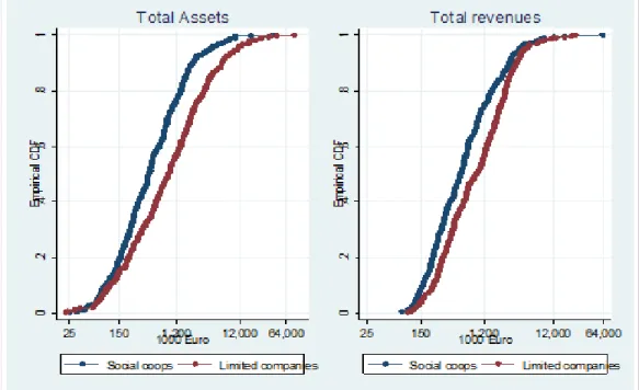
corresponding to the residential social services, i.e. firms operating nursing homes for the elderly, disabled, patients with psychiatric disorders or drug addicts. We are able to find 800 companies with 2009 balance sheet data satisfying the previous criteria. Among them, 411 are share companies and the remaining 389 are social cooperatives4: we consider the former as our sample of for-profit companies (and below we refer to them as Limited companies) and the latter as nonprofit (SCs below). Companies are remarkably heterogeneous with respect to their size, both between and within the two types of firms we consider. In Figure 1 we depict the empirical distribution function of total assets and total revenues by company type. The median limited liability company has 0.89 million Euro of total assets in 2009, the double of the median social cooperative. As the graph shows, only 25% of not-for-profit companies have more than 1.1 million Euro of total assets. The right graph of Figure 1 shows that SCs are smaller than limited companies also in terms of total revenue (with a median of 0.58 vs. 1.03 million Euro).

Companies look somewhat more homogeneous if we consider few fundamental indexes which play a crucial role in our empirical analysis. First, we consider C(p*,k*) to be the stock of assets (either tangibles or not) used by the company to supply its services. We then introduce the leverage, defined as the ratio between total debt and total assets. We consider such a variable as a proxy of the theoretical L*. The Return on Assets (ROA) index is defined as the ratio between profits gross of taxes and total assets, a proxy of the expected return of one unit of investment. Finally, the Tangible Assets/Total Assets ratio is, given the dimension of the company, a proxy of the amount of collateral the company can provide to the lender and potentially positively correlated with the leverage.

Figure 1 - Distribution of total assets and total revenues by company type - Year 2009

Table 1 shows that on average the limited companies have the highest leverage together with the highest tangible to total assets ratio and the highest ROA. It is worth remarking that, although we consider firms operating in the same sector, their

activities may differ substantially. Such dissimilarities are not directly observable but might be reflected by the incidence of the labour cost on the revenues. We thus consider the Labour costs/Total Revenues ratio as a useful index to describe these structural differences: in Table 2 below we show that this ratio is remarkably higher for the SCs than for the for-profit companies. These statistics suggest that the firms in our sample supply heterogeneous services, with SCs specializing in labour intensive ones.

Table 1 - Ratios by company type, averages over the 2000-2009 period. Percentage points Social cooperatives Limited companies

Leverage 58.04 70.87

ROA 3.74 4.63

Tangible/Total Assets 19.83 34.82

Labour cost/Total revenue 55.72 35.94

Standard error ROA 6.79 6.05

Financial burden/Total Debt 1.97 2.91

Years operating 11.43 11.84

Number of observations 2207 2365

The decision to resort to the credit market is related to the risk aversion of the entrepreneurs which, again, is not directly observable. A risk-averse agent is ready to accept a lower expected return on investment in order to reduce its volatility. We can therefore compare the mean and the standard error of ROA for the two types of companies to gain some insight into their risk attitude. Table 1 shows that the mean of ROA is lower for the SCs, while the mean of the ROA standard error over the period considered is lower for the SCs, which suggests that not-for-profit firms are more risk tolerant than for-profit companies.

Finally, if we consider the financial burden/total debt as a proxy of the credit cost, we see that SCs have on average a financial burden lighter than that of the limited liability companies; we conclude that credit is likely to be less costly for social enterprises.

4. Regression analysis

In this section we run a multiple regression analysis by estimating a random effects model for longitudinal data (Wooldridge, 2001). This will give further insights into the effects of the variables considered in the theoretical model over the actual choices of the leverage operated by the companies. We have balance sheet information going from 2000 to 2009 and we follow a reduced form equation approach by estimating the following linear dynamic model

lnL_it = z_i′

α δ

+ ₁lnL_it−1 +

δ

₂lnL_it−2 +x_it′₋₁

β

+T_t′

γ ε

+ +_i u_it (18) where: lnL is logarithm of the leverage; zi is a set of time invariant company

characteristics including a dummy variable which equals 1 for the limited companies; xit includes total assets (in logs), the ratio of tangible to total assets, the incidence of

the labour costs on total revenue, and the ROA index; Tt identifies a full set of time

dummies in order to take into account business cycle effects; εi is the unobservable

time invariant individual effect; finally, uit is the idiosyncratic error term. Given

dynamic nature of the model under consideration, neither the ordinary least squares (OLS) nor the generalized least squares (GLS) provide consistent estimates of the parameters of interest. Indeed, past values of the balance sheet items are correlated with the unobservable time invariant characteristics of the firms, εi, and they are

potentially correlated with past idiosyncratic shocks, uit. We thus resort to GMM

estimates following Blundell and Bond (2000). We use time variant covariates lagged at least twice as our instrument for the first differenced equation; we instead rely on time, regional, industry and start up dummies for the level equation. The Sargan test for the overidentifying restrictions and the Arellano-Bond test for zero autocorrelation in first-differenced errors never reject the hypothesis of correct specification.

Variation in the level of debts, and more in general the capital structure of the company, is affected by some degree of inertia: our estimates (see Table 2) show that indeed the current leverage is positively correlated to its past values. Such correlation does not explain all the dynamics, the leverage decreases when the total assets increase and when the companies become more profitable. Although the parameter is precisely estimated, the economic relevance of this relation is limited: one percentage point more of ROA is associated with a decrease of 0.3% of the leverage, which at the average leverage level of 64.7% corresponds to 0.02 percentage points. The elasticity of leverage to total assets (∂lnLeveraget /∂lnTotalAssetst) is estimated to be -0.05.

The estimated parameter for the tangible to total assets ratio is 0.40, which suggests the access to the credit market is significantly affected by the nature (tangible vs. intangible) of the firms’ assets, and that the total amount of assets is not a sufficient descriptor of the company ability to put up a collateral. Unsurprisingly, the past values of the leverage ratio plays a crucial role: one percent increase in the last year leverage determines a 0.32% increase in the leverage of the following year, which corresponds on average to an increase of 0.2 percentage points. The incidence of labour costs on total revenue does not seem to significantly affect the indebtedness of the company. Finally, although we controlled for many observable characteristics of the companies, the for-profit companies proved to have a leverage 18% higher than SCs. This difference is reduced only when we compare start up coops with limited companies operating for more than 5 years.

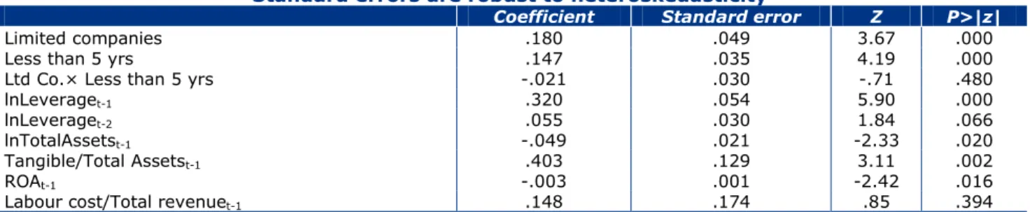
Table 2 - GMM estimates of equation (18). Dependent variable: leverage. The specification includes also year, regional and industry dummies.

Standard errors are robust to heteroskedasticity

Coefficient Standard error Z P>|z|

Limited companies .180 .049 3.67 .000

Less than 5 yrs .147 .035 4.19 .000

Ltd Co.× Less than 5 yrs -.021 .030 -.71 .480

lnLeveraget-1 .320 .054 5.90 .000

lnLeveraget-2 .055 .030 1.84 .066

lnTotalAssetst-1 -.049 .021 -2.33 .020

Tangible/Total Assetst-1 .403 .129 3.11 .002

ROAt-1 -.003 .001 -2.42 .016

Labour cost/Total revenuet-1 .148 .174 .85 .394

Why do the limited companies have a capital structure different from SCs even after controlling for all the above factors? According to our theoretical framework, SCs, being more oriented towards consumer welfare, reduce the price. This increases their demand and, in turn, their production costs: a cash-constrained firm is therefore forced to increase borrowing. At the same time the presence of a non-distribution constraint, peculiar of nonprofit organizations, increases the fraction of own capital on total investment: this negatively affects leverage of SCs according to Proposition 1. Our main empirical finding is that leverage of for-profit companies is 18% higher than that of SCs. After remarking that credit is likely to be less costly for social enterprises as indicated in Table 1, the empirical result is interpreted by conjecturing that negative effect of the non-distribution constraint on leverage outdoes positive one due to consumer orientation.

Appendix

A.1 Optimal price (13) Focus on (12): notice that

a+bc-(2a+bc)α+bcr(1-k)(1-α)≥0⇔α≤((a+bc(1+r(1-k)))/(2a+bc(1+r(1-k))))

and

-bp(2-3α)≥0⇔α>(2/3)

where ((a+bc(1+r(1-k)))/(2a+bc(1+r(1-k))))<(2/3) under Assumption 1.

It follows that for α∈(((a+bc(1+r(1-k)))/(2a+bc(1+r(1-k)))),(2/3)], (12) is negative, hence

the optimal price is minimum, p=c. By contrast if α≤((a+bc(1+r(1-k)))/(2a+bc(1+r(1-k)))), then the F.O.C. gives

p=((a+bc(1+r(1-k))-(2a+bc(1+r(1-k)))α)/(b(2-3α))) (19)

In this interval both the S.O.C. ((∂²)/(∂p²))=-b(2-3α)<0⇔α<(2/3) is verified. We have ((a+bc(1+r(1-k))-(2a+bc(1+r(1-k)))α)/(b(2-3α)))≥c(1+r(1-k))⇔(1/2)≥α.

Moreover, (1/2)<((a+bc(1+r(1-k)))/(2a+bc(1+r(1-k)))). Finally, if α>(2/3) the F.O.C. rewrites gives

p=(((2a+bc(1+r(1-k)))α-(a+bc(1+r(1-k))))/(b(3α-2))) (20)

where (((2a+bc(1+r(1-k)))α-(a+bc(1+r(1-k))))/(b(3α-2)))>(a/b) and the S.O.C. is not verified. We can correctly state that (20) is a minimum point higher than the upper bound

(a/b) on p. It follows that (12) is negative in α>(2/3), for which interval the optimal price is

minimum, p=c. These findings are summed up by (13).

A.2 Optimal leverage (17) Note that

((∂k∗_{)/(∂α))=-(M/(c(1-α)√(4Mbr(2-3α)(1-α)+(1-α)²(a-bc(1+r))²)))<0}

for α∈[0,(1/2)), while ((∂k∗_{)/(∂α))=0 for α∈[(1/2),1]. It follows that L}∗ _{is minimum for α=0 and}

equal to

1-((√(c²(a-bc(1+r))²+8bc²rM)-c(a-bc(1+r)))/(2bc²r)).

Such a value is strictly higher than 0 if and only if M<((c(a-bc))/2), in which case L∗>0 for any α. On the contrary, L∗ _{is maximum for α≥(1/2) and equal to}

1-((√(c²(a-bc(1+r))²+4bc²rM)-(c(a-bc(1+r))))/(2bc²r)).

Such a value is strictly lower than 0 if and only if M>c(a-bc), in which case L∗=0 for any α.

Finally, we solve by α the following inequality to compute optimal leverage of a firm with cash holding M∈[((c(a-bc))/2),c(a-bc)]:

((√((1-α)(4rbM(2-3α)+(a-bc(1+r))²(1-α))))/(2bcr(1-α)))-((a-bc(1+r))/(2bcr))≥1

and get α≤((2M-c(a-bc))/(3M-c(a-bc))), where M∈[((c(a-bc))/2),c(a-bc)] implies that ((2M-c(a-bc))/(3M-c(a-bc)))∈[0,(1/2)].

References

Blundell R., Bond S. (2000), “GMM Estimation with Persistent Panel Data: An Application to Production Functions”, Econometric Review, 19(3), pp. 321-340.

Bonatti L., Borzaga C., Mittone L. (2005), “Profit Versus Non-profit firms in the Service Sector: An Analysis of the Employment and Welfare Implications”, Rivista di Politica Economica, 95 (3), pp.137-164.

Borzaga C., Depedri S., Tortia E. (2010), The Growth of Organizational Variety in Market

Economies: The Case of Social Enterprises, Euricse Working Papers No. 003/10.

Brekke K., Siciliani L., Straume O.R. (2011), Quality Competition with Profit Constraints: Do

Non-profit Firms Provide Higher Quality than For-profit Firms?, CEPR Discussion Paper No.

8284.

De Fraja G., Delbono F. (1990), “Game Theoretic Models of Mixed Oligopoly”, Journal of

Economic Surveys, 4, pp. 1-17.

Fedele A., Miniaci R. (2010), “Do Social Enterprises Finance Their Investments Differently from For-profit Firms? The Case of Social Residential Services in Italy”, Journal of Social

Entrepreneurship, 1 (2), pp. 174-189.

Kitzmueller M., Shimshack J. (2012), “Economic Perspectives on Corporate Social Responsibility”, Journal of Economic Literature, 50(1), pp. 51-84.

Nett L. (1993), “Mixed Oligopoly with Homogeneous Goods”, Annals of Public and Cooperative

Economics, 64, pp. 367-393.

Wooldridge J.M. (2001), Econometric Analysis of Cross Section and Panel Data, MIT Press, Boston.