Research Article
Analysis of Reactive Injection Compression Molding by Numerical
Simulations and Experiments
Giorgio Ramorino , Silvia Agnelli, and Matteo Guindani
Department of Mechanical and Industrial Engineering, University of Brescia, Via Branze 38, 25123 Brescia, Italy
Correspondence should be addressed to Giorgio Ramorino; [email protected] Received 9 August 2019; Accepted 22 January 2020; Published 18 February 2020 Academic Editor: Thomas J. Farmer
Copyright © 2020 Giorgio Ramorino et al. This is an open access article distributed under the Creative Commons Attribution License, which permits unrestricted use, distribution, and reproduction in any medium, provided the original work is properly cited.
Injection compression molding is an injection molding process with the addition of a compression stage after the injection. This process is useful for the injection molding of precision parts. A stable and controlled manufacturing process is needed to guarantee reliability of complex products, and usually process optimization is achieved by experimental and time consuming approaches. However, for being competitive a minimal market time is a very important requirement and computer simulations can help to optimize the process at the only expense of computational time. This paper reports and discusses for the first time the results of a 3D finite element simulation of reactive injection compression molding (RICM) by commercial software for the production of rubber diaphragms. In particular, the stages of mold filling dynamics and material curing are analyzed and the results verified with experimental tests. To get an accurate representation of the process, the rheological behavior, thermal properties, and kinetic behavior during curing of the real rubber compound were de-scribed by mathematical models. A differential scanning calorimeter (DSC) and a capillary rheometer are employed to characterize the rubber material in order to achieve an appropriate curing reaction and viscosity models, respectively. The computations are found to be in good agreement with the experimental results, indicating that reliable information on material viscosity and curing kinetics can play a key role in making well-founded predictions and avoiding trial and error methods.
1. Introduction
Many rubber articles are produced by molding, a process in which uncured rubber, sometimes with an insert of plastic or metal, is cured under pressure in a mold. Determining the right process for part production is a crucial step in the ultimate success of a product. There are three general molding techniques for rubber: compression, transfer, and injection molding. The choice of the best process is based on a number of key factors, including: the size and shape of the part, the hardness, flow and cost of the material, and the number of rubber parts to be produced [1–3].
Injection compression molding (ICM) [4] is a molding process which combines conventional injection molding and compression molding and has been developed to incorpo-rate the advantages of both molding processes.
Rubber compression molding (RCM) [5, 6] is a process where preheated rubber is placed in a heated mold cavity (single or multicavity). Once closed off or reassembled, pressure is applied to the mold forcing the rubber material into contact with all internal surface areas. Then the heat and pressure are continuously applied until the rubber has cured. Compression molds vary considerably in size, shape, and complexity and also contain from one to a very high number of cavities. Compression molding is often chosen for me-dium hardness compounds–in high volume production or in applications requiring particularly expensive materials. It requires inexpensive tooling but it is a labor-intensive process with loading and process times longer than other molding methods.
Rubber injection molding (RIM) [7] is normally the most automated of the molding processes. The material is
Volume 2020, Article ID 1421287, 8 pages https://doi.org/10.1155/2020/1421287
heated to a flowing state and injected under pressure from the heating chamber through a series of runners or sprues into the mold. Generally, parts manufactured using injection molding need additional treatments such as cryodeflashing and surface treatments to reduce the coefficient of friction. However, with some types of moulds it is possible to obtain finished parts that do not require additional finishing. The process is used for high production runs and parts that require tighter tolerances.
The schematic of the RICM (rubber injection com-pression molding) process used in this work is illustrated in Figure 1. Before the injection stage, the thickness of the mold cavity is set to be slightly larger than the nominal thickness of the part. This thicker cavity allows the polymer melt to flow into the mold cavity under low injection pressure. By closing the mold halves, the mold cavity thickness is reduced to the final part thickness. Injection compression molding has the advantages of decreasing molding pressure, reducing re-sidual stress, minimizing molecular orientation, even packing, reducing uneven shrinkage, preventing sink marks and warpage, reducing density variation, and increasing dimensional accuracy.
Because of these advantages, injection compression molding is often employed to produce plastic parts of high accuracy dimensions and free of residual stress, especially for optical components [8–17]. However, the simulation of injection compression molding is very challenging due its complexity in terms of material data and process sequence. For the first time, this paper shows the results of a simulation of RICM process for rubber components.
Given that the rubber exhibits extremely complicated thermoviscoelastic material properties, the complexity of the model process makes it very challenging to attain the desired properties of parts and thus it is difficult to maintain part quality during production. One way researchers have found to improve the efficiency of this process is Computer Aid Engineering (CAE). Computer simulations allow increasing the final quality of the product by the correct selection of the technological parameters during rubber processing and, at the same time, obtaining significant savings by the project of an adequate period of the production cycle. In spite of the relevance of this tool, there are no literature works on the simulation of the RICM process for rubber.
This paper reports and discusses for the first time the results of the 3D finite element simulation of reactive in-jection compression molding (RICM) for the production of rubber diaphragms. Simulation is carried out using the “Reactive Molding” module of the Autodesk Moldflow 2018 CAE software, and the results are validated via the com-parison with experimental tests. A very thin rubber dia-phragm with complex geometry used in engineering was selected for this study. The mold filling dynamics in the injection and compression stages during the processes were analyzed. The representation of the filling progress is one of the most important outputs in order to identify weld lines and places where air bubbles may form. Finally, processing conditions, including compression stroke and compression speed, were investigated with a view to reducing the cavity pressure.
A successful injection molding simulation requires understanding of the actual material behavior and its de-scription in the simulation using suitable material models. Because of the complex formulation of rubber compounds and the high degree of customization, there are problems associated with the use of existing material data sets from commercially available databases. For this reason, proper measurements of material viscosity and curing rate are required in order to run a simulation. A differential scanning calorimeter (DSC) and a capillary rheometer are employed to characterize the rubber material in order to obtain ap-propriate curing reaction and viscosity models, respectively, following an experimental approach already developed by the authors for the simulation of injection molding process [18]. The model parameters thus obtained are used to simulate the injection compression molding process.
2. Experimental Characterization of
the Material
2.1. Material. In this study, the experimental investigations
are carried out on an acrylonitrile butadiene rubber (NBR). The compound with NBR with 33% of nitrile content, a sulphur-based curing system and 30 wt.% of carbon black, was provided by Ligom srl (Grumello del Monte, Bergamo, Italy). The specific compound formulation and preparation is not disclosed due to commercial reasons. The base ma-terial is indicated in this work as NBR60, since after com-plete vulcanization, it has a hardness of 60 Shore A and 59.4 IHRD. Hardness Shore A measurements were performed on 6 mm plates, according to ISO 7619-1:2010. IRHD hardness measurements were performed on 2 mm plates, according to ISO 48:2010.
2.2. Rheological Characterization. In order to characterize
the rheological behavior, the flow curves of the rubber compound were obtained at different temperatures by a Rheologic 5000 Twin-Bore capillary rheometer by CEAST. Rheological measurements were performed with the NBR compound prepared without curatives, to avoid obstruction of the capillaries, particularly at high temperatures. The apparent viscosity data versus the apparent shear rate data were calculated for temperatures of 130, 150, and 170°C.
Bagley [19] and Rabinowitsch [20] corrections were applied to calculate the adjusted viscosity data.
The reactive viscosity model [18, 21–23] is used to de-scribe the rheological properties of rubber compounds in the Plastics Insight (MPI) Reactive Molding Moldflow software in order to simulate the mold filling dynamics. The Reactive Viscosity Model is given by
η � η0(T) 1 + η 0(Tc)/τ∗ (1− n)× αg αg− α C1+C2α , (1) η0� Bexp Tb T , (2)
whereƞis viscosity,ƞ0is “zero viscosity,” that is, viscosity at
level at the transition between Newtonian and power law regions, α is the degree of cure, agis the degree of curve at gelation point, C1and C2are fitting parameters, B and Tbare
fitting parameters, and T is the temperature. The terms C1
and C2were set to 1 and 0 on the basis that the rubbers used
in this work did not cure during the filling phase. α is the degree of cure, and the gelation conversion (ag) was set to 0.1 as a default value.
The parameters τ∗, n, B, and T
bwere calculated using
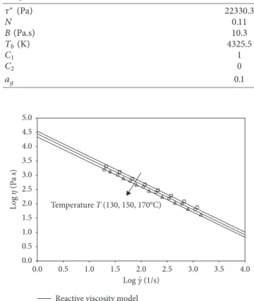
Origin software. Since the rheological tests were performed on compounds without cross-linking agents, only the pa-rameters concerning the shear rate dependence of viscosity were determined from the experimental data. It should be pointed out that experimental viscosity data were measured in a range of logarithmic shear rate from about 1.3 to 3 1/s, the typical range of the capillary rheometer. This experi-mental method was chosen since it is able to simulate the process conditions of high shear rate, pressure, and high shear exerted on the compound during the injection phase and during the final stages of mold closure. Moreover, as in the injection phase, the flow in the capillary is (nearly) fully developed, and the filler-filler structures are destroyed. Probably the simulation could be even more accurate adding viscosity data at lower strain rates. However, to obtain such data other types of experimental tests should be performed, such as dynamic mechanical tests, which however do not reproduce the fully developed flow. Therefore, in this work it was decided to keep the characterization as simple as pos-sible. Deeper understanding could be obtained with other test methods; this will be the topic of future works.
Table 1 indicates the values obtained for these param-eters and Figure 2 shows the good agreement between the experimental sets of data of viscosity, evaluated at different shear rate values and at temperatures of 130, 150, and 170°C
(open symbols) and the respective curves generated by the Reactive Viscosity Model (lines).
2.3. Cure Kinetics Characterization. The curing of the
ma-terial was defined in terms of the induction and cure kinetics and was experimentally characterized by DSC analyses. DSC analysis is an alternative technique to curemeter methods, as pointed out in previous literature works [24, 25]. Heat Flux DSC from TA Instruments was used. Isothermal tests were performed at 140, 150, 160, and 170°C. This test generates a
profile of dQ/dt versus time. The induction time is assumed to be the time at which the baseline cuts the exotherm curve.
During this time, no chemical reaction takes place inside the rubber. The degree of cure (from 0 to 1) can be calculated using the following equation:
α(t) �ΔHt
ΔHT
. (3)
The data of ti(T), obtained from each isothermal DSC
test, are used to obtain the two constants (B1and B2) of the
Claxon-Liska model to characterize the induction time of the NBR compound [26, 27]:
ti(T) � B1exp(B2/T0). (4) The rate of cure values (dα/dt) as a function of cure degree α shown in Figure 3 is easily calculated from the plots of α versus t (cure kinetics curve) shown in Figure 4.
(a) Initial compression gap (b) Polymer melt injected into a pre-enlarged cavity
(c) Polymer melt compressed by clamping movement of machine
Figure 1: Schematic of the RICM process.
Table 1: Parameters of the reactive viscosity model for the NBR60 compound. τ∗(Pa) 22330.3 N 0.11 B (Pa.s) 10.3 Tb(K) 4325.5 C1 1 C2 0 ag 0.1 Temperature T (130, 150, 170°C) L og η (P a s)
Reactive viscosity model 0.0 0.5 1.0 1.5 2.0 2.5 3.0 3.5 4.0 4.5 5.0 4.0 3.5 3.0 2.5 2.0 1.5 1.0 0.5 0.0 Log γ (1/s).
Figure 2: Experimental data of viscosity, evaluated at the tem-peratures of 130, 150, and 170°C (open symbols) and the respective
These data are used to obtain the constants of the Kamal-Sourour model [28] to characterize the cure kinetics of the material. In fact, Kamal and Sourour proposed that
dα dt � K1+ K2α m (1 − α)n, (5) K1� A1exp − E1 RT , K2� A2exp − E2 RT , (6)
where K1and K2are functions of the temperature and are
defined by m, n, E1, and E2 parameters. m and n are
reaction orders; E1and E2are the activation energies; R is
the gas universal constant parameter, with a value of 8.31 J (mol ∗ K). Data measured from DSC tests were fitted to this model with Origin software and reported in Table 2.
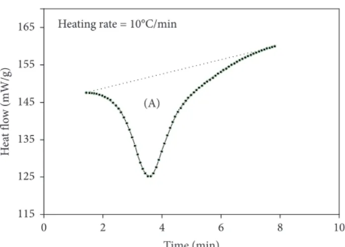
The model parameters reported in Tables 1 and 2 are used to simulate the injection molding process including the stages of the mold filling dynamics and material curing of the rubber component. To evaluate the specific heat of reaction, nonisothermal DSC scans are taken at a fixed heating rate of 10°C/min within the temperature range 70–220°C. A typical
DSC trace is shown in Figure 5 where an exothermic re-action peak is observed. The specific heat of rere-action H (J/g), as determined by the value of the peak area (A) divided by the mass of the sample (about 16 mg), is H � 11.64 J/g.
Thermal conductivity of the NBR compound is taken equal to 0.4 W/m/K and is calculated as average value of thermal conductivities reported both in the literature and in the software database for NBR compounds.
3. Simulations and Discussions
3.1. Part Geometry and Simulation by CAE (Computer Aided Engineering). The geometry of the rubber diaphragm part
shown in Figure 6(b) is obtained after trimming the molded shoot (mold cavity) shown in Figure 6(c). This component is characterized by a complex geometry with a thickness distribution that ranges from 0.18 mm to 0.85 mm. The 3D-CAD drawing of the multicavity mold was exported to the FE software in STEP format and modelled using Autodesk Moldflow 2018.
In the numerical modeling and simulation, a circular sector with an angle of 90°is chosen as the computational
domain. Since the geometry of the component is circular and the injection location is exactly in the centre, a radial filling is expected. In order to limit the number of elements and thus the calculation time, we chose to simulate just a slice of the part. The slice was chosen large enough to be representative of the filling of the entire part; therefore, with the exception of the lateral boundaries of the slice, the filling in it can be considered as axisymmetric for the other slices of the part. Figure 6(d) shows the computational domain with the relative boundary conditions. In compression type molding process simulations, the surface of the model must be assigned the “compression surface” property type so the software can identify where compression will occur. The compression (moving) surface, green in Figure 6(d), is considered to be the press side of the cavity and will follow the press movement exactly while the fixed surface (yellow in Figure 6(d)) is considered to be the fixed side of the cavity. No movement occurs during compression. The domain is discretized by about 1,500,000 tetrahedral elements (Figure 6(a)) with minimum 6 elements in the thickness
Temperature T (140, 150, 160, 170°C)
dα
/d
t
Experimental data Cure kinetics model 0 0.002 0.004 0.006 0.008 0.01 0.012 0.014 0.016 0 0.2 0.4 0.6 0.8 1 α
Figure 3: The rate of cure values (dα/dt) as a function of cure degree evaluated at different temperatures (― experimental data; --- curve generated by cure kinetics model).
Temperature T (140, 150, 160, 170°C) α 0 0.2 0.4 0.6 0.8 1 1.2 50 100 150 200 250 300 350 400 0 Time (s) Experimental data
Figure 4: Cure kinetics curves: cure degree α as a function of time (s) evaluated at different temperatures (140, 150, 160, and 170°C).
Table 2: Cure parameters defined for the NBR compound.
B1(s) 1.2 × 10 −5 B2(s) 6642 A1(s−1) 0 E1/R (K) 0 A2(s−1) 4.26 × 10⁸ E2/R (K) 10082 M 0.535 N 1.273
direction, which has been selected after a mesh statistics test. For a given compression speed, the mesh system is deformed and a new configuration is formed at every time stage. Then the nodal coordinate values and other auxiliary quantities are updated to obtain new velocity, pressure, and temper-ature, at each time stage.
3.2. Process Settings. In the reactive compression-injection
process, the cavity thickness is initially greater than the target thickness and the rubber is injected into the cavity at a user-defined injection velocity. At the velocity-pressure switchover time, the pack phase starts, following a user-defined packing profile, and regardless of when press compression is programmed to start. Meanwhile, the press is moved to a predetermined position. It will be stationary and stay in this position for a period of time. The waiting time starts when the injection begins and ends when the press
begins to move. The compression stage starts when the press begins to move. In the press compression stage, the movement of the press initially takes place under speed control, specified by the press compression speed at in-cremental distances profile. The press can keep moving forward; however, it will be in a constant force control mode (preset force). Finally, after the press compression phase is Heating rate = 10°C/min
0 2 4 6 8 10 Time (min) 115 125 135 145 155 165 H ea t f lo w (mW/g) (A)
Figure 5: Trace of a DSC thermogram obtained at a heating rate of 10°C/min within the temperature range 70–220°C for NBR compound.
Injection location Injection location (a) (c) (b) (d) Fixed Moving 1.6 22 0.18 0.85
Figure 6: (a) 3D mesh of the circular sector with an angle of 90°; (b) geometry of the rubber diaphragm (dimensions in (mm)); (c) 3D representation of the complete injection shot (mold cavity); (d) compression moving (green) and fixed (yellow) surfaces.
Table 3: Main process parameters.
Injection time (s) 2
Injection temperature (°C) 70
Mold temperature (°C) 170
Cure time (s) 210
Press open distance (mm) 6.3
Volumetric flow rate (injection) (cm3/s) 13.2
Press compression speed (mm/s) 3
Press compression start (% volume filled) 100
completed, the press will stay in that position and remain stationary for the specified curing time.
In order to verify the reliability of the flow simulation, the results of the simulation were compared to the results of experimental tests carried out under the same conditions of industrial production. In particular, a 300-ton MIR hori-zontal molding machine was used for the experiments. The same parameters used in the experimental test, including compression speed, switch time from injection to com-pression, and compression stroke, were used also in the simulation. Table 3 shows the main process parameters used for the computer simulations. The initial melt temperature is 70°C, the mold temperature is 170°C, and the initial press
open distance is 6.3 mm. Both initial melt and mold tem-perature were experimentally checked with a thermocouple. Melt temperature, measured on rubber purging, was in the range 70 ± 4°C, and mold temperature was measured in
several locations and resulted to oscillate in the range 170 ± 3°C. The temperature variations were hypothesized to
have negligible effects on the results of the simulation; therefore the average temperature values were set as pa-rameters. The press moves at a constant speed (at 3 mm/s) until switch over to force control. The volumetric flow rate for the injection phase equals 13.2 (cm3/s).
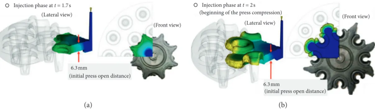
3.3. Mold Filling Dynamic. In Figure 7, we compare the
results of the filling patterns obtained from Moldflow simulation (Fill Time) and the corresponding incomplete molded part obtained through interrupted filling
experiments at the initial press open displacement of 6.3 mm. The Fill Time shows the position of the flow front at regular intervals as the cavity fills. The amount of melt inside the cavity before compression was set in advance, so that the volume of the material would be exactly the same as the part volume. A movable mold wall was used to compress the melt, which had previously partially filled in the cavity. As mentioned earlier, one of the most important outputs is the representation of the filling progress in order to identify weld lines and places where air bubbles may form.
Figure 8 shows the comparison between the pictures of the incomplete molded parts and the corresponding filling patterns predicted by computer simulation during the compression phase and the respective weld-line position (WL1 and WL2). The agreement appears remarkable,
sug-gesting that the predictions are representative of the flow during the filling stage. Figure 9 shows the final condition at the end of press compression and the real part obtained after trimming.
3.4. Curing Kinetics. In order to compare the results in terms
of curing kinetics, the experimental degree of cure of the component after injection molding was experimentally evaluated by DSC. Interrupted filling experiments were carried out at various cure times. Parts were taken out of the mold, and specimens were cut out from parts in zones defined as A in Figure 10. The specimens were analyzed by nonisothermal DSC scans with the same conditions of the
6.3 mm
(initial press open distance) Injection phase at t = 1.7s (Front view) (Lateral view) (a) Injection phase at t = 2s (Front view) (Lateral view)
(beginning of the press compression)
(initial press open distance) 6.3 mm
(b)
Figure 7: Results of the filling patterns obtained from simulation (Fill Time) and the corresponding incomplete molded part obtained through interrupted filling experiments at 1.7 s (a) and 2 s (b) of Fill Time. In both cases, the initial press open distance is 6.3 mm.
5.1 mm (press displacement = 1.2 mm) Compression phase at t = 2.4s WL1 WL1 Weld line (WL1) (Lateral view) (Front view) (a) Weld line (WL2) WL2 WL2 3.1 mm (press displacement = 3.2 mm) (Lateral view) (Front view) Compression phase at t = 3.1s (b)
Figure 8: Results of the filling patterns obtained from simulation (Fill Time) and the corresponding incomplete molded part obtained through interrupted filling experiments during the compression phase. The initial press open distance is 1.2 mm (a) and 3.2 mm (b).
uncured sample (see paragraph 2.3). The degree of cure was calculated with the following relationship:
α � ΔHt1− ΔHt2
ΔHt1
, (7)
where α is the degree of cure, ΔHt1is the exothermicity for
the uncured sample, and ΔHt2is the exothermicity of the
sample cured during time t.
If the sample is completely cured, the enthalpy will be zero, whereas for partially cured samples, an intermediate value will be obtained. The results of comparisons of the experimental cure curve with that predicted by simulations are shown in Figure 10; measurements were made only in zones defined as A. The experimental points are measured at times compatible with experimental practice: usually ponents are undercured and the curing reaction is com-pleted in a postcuring phase out of the mold. Therefore the risk of reversion and of consequent decay of rubber prop-erties is prevented both by the short process times and by the material, which does not show reversion. It was clearly observed that the cure kinetics predicted by the simulations showed faster cure profiles than those obtained in reality. In any case, to obtain good vulcanization, assumed as 90% average degree of cure, the software predicts 92 s, which is in
good agreement with the data obtained through the DSC test (100 s).
4. Conclusions
The injection compression molding process for rubber di-aphragms, including the stages of the mold filling dynamics and material curing, was modelled virtually for the first time. The virtual results were verified in real injection molding tests. A process optimum was successfully found that en-sures both component quality and the highest possible economic efficiency. The simulation turned out to be a reliable and effective tool to predict potential defects as weld lines. Correct measurement and modeling of the material behavior were essential for successful use of the model. Further improvements in the approach could further im-prove the accuracy of results. The imim-provements concern the following parameters: (i) boundary conditions, such as mold and melt temperature, whose variability could be taken into account in the simulation; (ii) experimental viscosity characterization covering also low shear rate values, to better simulate the compression phase; and (iii) mold surface roughness, which could affect filling phase particularly in case of thin sections.
Data Availability
The experimental and numerical data used to support the findings of this study are available.
Conflicts of Interest
The authors declare that there are no conflicts of interest regarding the publication of this paper.
Acknowledgments
The research was financially supported by the University of Brescia, Department of Mechanical and Industrial Engineering.
References
[1] M. R. Kamal and M. E. Ryan, Injection and Compression
Molding Fundamentals, A. I. Isayev, Ed., Marcel Dekker, New
York, USA, 1987.
[2] J. A. Lindsay, Practical Guide to Rubber Injection Moulding, Smithers Rapra Technology, Shrewsbury, UK, 2012. [3] V. Walworth, Rubber Molding Principles, TechnoBiz
Com-munication Co., Ltd., Bangkok, Thailand, 2013.
[4] O. Solorza-Nicolas, H. Hernandez-Moreno, O. Susarrey-Huerta, and N. Romero-Partida, “Film-insert injection compression molding for reinforced polycarbonate with woven glass fiber oriented 90/0°, ±45°,” Polymer Engineering and Science, vol. 59, no. 2, pp. E372–E379, 2019.
[5] K. Maghsoudi, G. Momen, R. Jafari, and M. Farzaneh, “Direct replication of micro-nanostructures in the fabrication of superhydrophobic silicone rubber surfaces by compression molding,” Applied Surface Science, vol. 458, pp. 619–628, 2018. [6] K. Maghsoudi, G. Momen, and R. Jafari, “Micro-nano-structured silicone rubber surfaces using compression (92 s)
CAE prediction (90% degree of cure at point A)
(A) 20 40 60 80 100 120 140 160 180 200 220 0 Time (s) 0 0.1 0.2 0.3 0.4 0.5 0.6 0.7 0.8 0.9 1 Degree of cure α Experimental data
Figure 10: Comparisons of simulated degree of cure α versus time with that obtained from experimental measurements (measure-ments were made only in zones defined as A).
FINAL RUBBER COMPONENT: NBR DIAPHRAGM (end of the press compression)
(Trimming line) Compression phase at t = 4s (Lateral view) (a) (b) (c) 0.3 mm (press displacement ≈ 6 mm)
Figure 9: Final condition at the end of press compression (a) and the real part (c) obtained after trimming the molded part (b).
molding,” in Proceedings of the Thermec 2018: 10th
Interna-tional Conference on Processing and Manufacturing of Ad-vanced Materials, vol. 941, pp. 1802–1807, Paris, FRANCE,
July 2018.
[7] K. Kyas, M. Stanek, D. Manas et al., “Novel trends in rheology V,” Book Series: AIP Conference Proceedings, vol. 1526, pp. 142–147, 2013.
[8] F. J. Parker, “Efficient processing of thermosets by injection moulding,” Plast Rubber Process, vol. 3, no. 1, pp. 24–28, 1978. [9] R. H. Schlueter, “Injection moulding methods,” European
Rubber Journal, vol. 164, no. 8, pp. 49–52, 1982.
[10] R. H. Schlueter, “Injection molding: review of non-traditional techniques and concepts,” Elastomerics, vol. 113, no. 12, pp. 37–41, 1981.
[11] B. Friedrichs, M. Horie, and Y. Yamaguchi, “Simulation and analysis of birefringence in magneto-optical discs: part A—formulation,” Journal of Materials Processing and
Manufacturing Science, vol. 5, no. 2, pp. 95–113, 1996.
[12] B. Fan, D. O. Kazmer, R. P. Theriault, and A. J. Poslinski, “Simulation of injection-compression molding for optical media,” Polymer Engineering & Science, vol. 43, no. 3, pp. 596–606, 2003.
[13] M. R. Kamal, A. I. Isayev, S. J. Liu, and J. F. Agassant, Injection
Molding: Technology and Fundamentals, Hanser, Cincinnati,
OH, USA, 2009.
[14] W. Michaeli, S. Hessner, F. Klaiber, and S. Hebner, “Analysis of different compression-molding techniques regarding the quality of optical lenses,” Journal of Vacuum Science &
Technology B: Microelectronics and Nanometer Structures,
vol. 27, no. 3, p. 1442, 2009.
[15] S.-C. Chen, Y.-C. Chen, H.-S. Peng, and L.-T. Huang, “Simulation of injection-compression molding process, part 3: effect of process conditions on part birefringence,”
Ad-vances in Polymer Technology, vol. 21, no. 3, pp. 177–187, 2002.
[16] H.-S. Lee and A. I. Isayev, “Numerical simulation of flow-induced birefringence: comparison of injection and injection/ compression molding,” International Journal of Precision
Engineering and Manufacturing, vol. 8, no. 1, pp. 66–72, 2007.
[17] W. Michaeli and M. Wielpuetz, “Optimisation of the optical part quality of polymer glasses in the injection compression moulding process,” Macromolecular Materials and
Engi-neering, vol. 284-285, no. 1, pp. 8–13, 2000.
[18] G. Ramorino, M. Girardi, S. Agnelli et al., “Injection molding of engineering rubber components: a comparison between experimental results and numerical simulation,” International
Journal of Material Forming, vol. 3, no. 1, pp. 551–554, 2010.
[19] E. B. Bagley, “The separation of elastic and viscous effects in polymer flow,” Transactions of the Society of Rheology, vol. 5, no. 1, pp. 355–368, 1961.
[20] B. Z. Rabinowitsch, “ ¨Uber die viskosit¨at und elastizit¨at von solen,” Journal of Physical Chemistry A, vol. 145, p. 1, 1929. [21] Autodesk, Simulation Moldflow Insight, Fundamentals 2014,
Student Guide—Practice Manual, Ascent, Charlottesville, VA,
USA, 2013.
[22] Autodesk, Simulation Moldflow Insight, Advanced Flow 2014,
Student Guide—Theory and Concepts Manual, Ascent,
Charlottesville, VA, USA, 2013.
[23] J. M. Castro and C. W. Macosko, “Studies of mold filling and curing in the reaction injection molding process,” AIChE
Journal, vol. 28, no. 2, pp. 250–260, 1982.
[24] M. A. L´opez-Manchado, M. Arroyo, B. Herrero, and J. Biagiotti, “Vulcanization kinetics of natural rubber-orga-noclay nanocomposites,” Journal of Applied Polymer Science, vol. 89, no. 1, pp. 1–15, 2003.
[25] R. Ding, A. I. Leonov, and A. Y. Coran, “A study of the vulcanization kinetics of an accelerated-sulfur SBR com-pound,” Rubber Chemistry and Technology, vol. 69, no. 1, pp. 81–91, 1996.
[26] W. E. Claxton and J. W. Liska, “Calculation of state of cure in rubber under variable time-temperature conditions,” Rubber
Age, vol. 95, no. 5, p. 237, 1964.
[27] A. Arrillaga, A. M. Zaldua, and A. S. Farid, “Evaluation of injection-molding simulation tools to model the cure kinetics of rubbers,” Journal of Applied Polymer Science, vol. 123, no. 3, pp. 1437–1454, 2012.
[28] M. R. Kamal and M. E. Ryan, “The behavior of thermosetting compounds in injection molding cavities,” Polymer