Mapping urban ventilation corridors and assessing their impact upon the cooling effect of greening solutions

(1)

MAPPING URBAN VENTILATION CORRIDORS AND ASSESSING THEIR IMPACT

UPON THE COOLING EFFECT OF GREENING SOLUTIONS

A. H. M. Eldesoky 1, *_{, N. Colaninno} 2_{, E. Morello} 2

1_{Università IUAV di Venezia, Palazzo Badoer, San Polo 2468, 30125 Venice, Italy –}_{ahmed.eldesoky@iuav.it}

2_{Laboratorio di Simulazione Urbana Fausto Curti, Dipartimento di Architettura e Studi Urbani, Politecnico di Milano, via Bonardi 3,} 20133 Milano, Italy – (nicola.colaninno, eugenio.morello)@polimi.it

Commission IV, WG IV/10

KEY WORDS: Ventilation Corridors, Urban Morphology, Urban Canyons, Green Solutions, Urban Heat Island ABSTRACT:

Over the past decades, climate change has become among the top issues challenging cities worldwide, endangering the urban infrastructures and threatening the health of millions of people. Hence, climate action, both in terms of mitigation and adaptation to climate change, has become a priority for urban planning. This work introduces an example of the promising role that spatial analysis and statistical modelling, employing Geographical Information Systems (GIS) and freely available satellite and land-based data, can provide in supporting urban climate design and policymaking. In particular, this study puts special attention on the Urban Heat Island (UHI) phenomenon. Here, we first introduce a simple, but effective morphological-based approach for mapping potential ventilation corridors across cities of uniform built-up structure, as a common UHI mitigation measure. Then, we propose a methodology for assessing the relative role of these corridors in maximizing the impacts of green solutions upon lowering high temperature. Results show that even under very calm wind conditions, there is still an opportunity for maximizing the benefits of greening measures on the urban climate. Also, it has been demonstrated that green ventilation corridors are more effective during night-time when the UHI effect is peaked. The research findings are very promising, especially for cities where wind is a marginal potentiality.

1. INTRODUCTION

Over the past century, the earth has witnessed a significant and constant increase in accumulated heat (NOAA, 2018). In cities and urban areas, the Urban Heat Island (UHI) effect and extreme heat waves are striking much greater portion of earth’s urban population and threatening the health of millions of people worldwide. Hence, mitigation and adaptation to climate change are on the top issues of the global agenda and of the major concerns of local authorities in cities and towns. For instance, urban greening has been widely used as a common UHI mitigation measure to regulate the microclimate air temperature and improve the quality of the urban environment (Ruefenacht and Acero, 2017). Vegetation (both grass-covered and tree-covered) can extremely reduce the accumulation of the incoming solar radiation in urban areas due to the characteristics of its physical properties in terms of the high albedo and low admittance (Ruefenacht and Acero, 2017). It also provides shading (in case of trees), cleans and purifies air, regulates the water cycle, and enhances the overall resilience of cities. Green roofs and facades, green/cool pavements, tree-lined streets, urban farming, and green ventilation corridors are among the most extensively used greening measures in cities.

Urban ventilation corridors are often paths realized across the urban street infrastructure and kept open to facilitate the flow of cooled and fresh air from the countryside into the dense warm urban environment, regulating the microclimate air temperature and improving air quality (Gál and Unger, 2009; Ren et al., 2018; Wicht et al., 2017). Vegetation arrangement and selective planting along ventilation corridors (referred to as green ventilation corridors) can be of great benefit. Studies have shown that near-surface air temperature at one location can be strongly *_{Corresponding author}

influenced by the intensity and vigor of vegetation in the surroundings in case of increased airflow (Bernard et al., 2018; Zhang et al., 2019; Zhao et al., 2014). However, it is noteworthy that vegetation by itself can significantly reduce ventilation due to the increased surface roughness (e.g. in case of tall or dense arrangement of trees), and thus it should be placed carefully in urban areas. Moreover, in many urban environments it is not feasible to widely expand urban greening, as space has become scarcer and the built geometry is very complex. Thus, designing a proper network of green ventilation corridors requires a prior precise and handy description and manipulation of the morphology of the urban environment (Samsonov et al., 2015). Over the last two decades, the advances in Geographical Information Systems (GIS) together with the availability of freely available meteorological data and remote sensing imagery have been extensively applied to urban analysis, design, and planning; and contributed effectively in modelling the urban climate phenomena (Burian et al., 2002; Gál et al., 2009; Kropf, 1996; Samsonov et al., 2015). In particular, concerning the mapping of potential urban ventilation corridors, one can distinguish between two main approaches. On one hand, wind tunnel and Computational Fluid Dynamics (CFD) models are used to make accurate simulations of wind flows in complex urban environments (Ren et al., 2018). However, although they can provide reliable simulations and better understandings of urban ventilation conditions, they are cost intensive and time consuming. Moreover, they are not applicable to large areas or whole cities (Hsieh and Huang, 2016; Wong et al., 2010). On the other hand, GIS and remote sensing techniques are alternatively used to approximately model wind conditions based on surface roughness. In fact, the latter, is a major determinant of airflow patterns and can be estimated using either micrometeorological The International Archives of the Photogrammetry, Remote Sensing and Spatial Information Sciences, Volume XLIII-B4-2020, 2020

(2)

or morphometric methods (Gál and Unger, 2009; Oke et al., 2017; Wicht et al., 2017). Roughness length (𝑧𝑧𝑑𝑑), zero plane displacement height (𝑧𝑧0), and Frontal Area Index (FAI) are among the most used morphometric indicators to estimate surface roughness (Burian et al., 2002; Counihan, 1975; Grimmond and Oke, 1999; Lettau, 1969; Oke et al., 2017; Wong et al., 2010). For instance, Gál and Unger (2009) and Wong et al. (2010) developed GIS-based methods and employed a building database to calculate FAI and identify ventilation corridors across Szeged (Hungary) and Hong Kong city, respectively. Suder and Szymanowski (2014) and Wicht et al. (2017) alternatively combined remotely sensed data and GIS techniques to calculate roughness length (𝑧𝑧𝑑𝑑) and zero plane displacement height (𝑧𝑧0); and subsequently map potential ventilation corridors in Wroclaw and Warsaw (Poland), respectively. Other researchers have combined both CFD models and GIS techniques for better delineating and evaluating potential ventilation corridors (Chang et al., 2018; Chen et al., 2017; Hsieh and Huang, 2016). Even so, other urban geometric properties can alternatively offer promising opportunities for mapping potential ventilation corridors. For example, different patterns and velocities of airflow can be modelled based on street canyon orientations with respect to the airflow direction, e.g. helical flow, staked flow, and channeling (Belcher, 2005; Oke et al., 2017; Voogt and Oke, 1997).

Furthermore, assessing the cooling effect of different greening measures is a very important step before making decisions on vegetation implementation in urban areas. Although this can be accurately assessed using CFD simulations and detailed vegetation modelling, regression models (e.g. linear, multiple, Geographically Weighted Regression [GWR]) have proven to be effective and powerful tools in modelling the urban climate phenomena (Colaninno and Morello, 2019; Fabrizi et al., 2010; Ninyerola et al., 2000; Xu et al., 2012; Yan et al., 2009). For instance, the Normalized Difference Vegetation Index (NDVI) (Rouse et al., 1974) was proven to have a negative correlation with land surface and near-surface air temperature in many studies (Colaninno and Morello, 2019; Rasul et al., 2017; Weng et al., 2004). More specifically, GWR models, which account for spatial non-stationarity, have demonstrated to have a better goodness-of-fit and predictive performance when compared to global models in explaining the relationship between NDVI and surface or near-surface air temperature (Colaninno and Morello, 2019; Zhao et al., 2018).

Here, our goal is twofold. Firstly, we propose an alternative approach to using surface roughness indicators for mapping potential urban ventilation corridors, especially for cities or contexts where building heights information is not available. It relies on employing street canyon orientations or azimuthal directions to model airflow patterns. Secondly, we aim at assessing the effectiveness of relatively high potential ventilation corridors in maximizing the impact of greening measures upon lowering high temperatures in cities.

2. STUDY AREA AND DATA

The study area is the city of Milan, which covers a surface area of about 181.7 km² and has a population of around 1.37 million inhabitants. Being in the center of the Pianura Padana (Po Valley), Milan is characterized by a flat topography, hot humid summers, and cold damp winters, in addition to an annual average low wind speed of about 4 m/s. Furthermore, the city has a significant UHI intensity that was estimated in 2017 to be 1.1 °C and 2.1 °C of screen-height temperature difference between

urban and rural areas for daytime and night-time, respectively (Colaninno and Morello, 2019).

In this work, we used a 1-m Digital Elevation Model (DEM), retrieved from a high quality digital topographic database of building footprints, provided by Lombardy Region at regional level. In addition, we employed raster data for NDVI and near-surface air temperature (both daytime and night-time) at 30-m spatial resolution, for an extreme event, which was the 4th of August, 2017, as suggested by Colaninno and Morello (2019). More specifically, the NDVI is Landsat-based, which has a 30-m spatial resolution and is calculated as follows:

NDVI =(NIR − Red)_{(NIR + Red)} (1) where NIR = Near-infrared band

Red = Visible red band

The average wind speed for August 4, 2017 was 1.5 m/s and the average wind direction was Southwest (SW), which is in agreement with the prevailing wind direction during the summer season in the city of Milan.

3. METHODOLOGY 3.1. Mapping urban ventilation corridors

Three main steps were required for mapping potential urban ventilation corridors across the city of Milan, based on the canyon orientations or azimuthal directions. Firstly, canyon azimuthal directions were calculated using a raster-based approach. Then, patterns of increased airflow were modelled. Lastly, potential urban ventilation corridors were mapped using a Least Cost Path (LCP) analysis.

3.1.1. Calculating canyon orientations. Urban or street

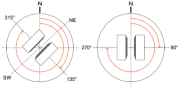
canyon orientation is usually defined by the cardinal direction in which the street runs, e.g. North-South (N-S), East-West (E-W), Northeast-Southwest (NE-SW), and Southeast-Northwest (SE-NW). In order to define canyon orientations, we applied Euclidean geometry to calculate the direction, in degrees, of the perpendicular line between the two boards of the canyon (building facades), measured clockwise from north, where, for example, a N-S-oriented canyon can have an azimuth angle equal to 90° or 270° and a NE-SW-oriented canyon has an angle equal to 135° or 315° (Figure 1).

Figure 1. The calculation of canyon azimuthal directions. A NE-SW-oriented canyon (left) and a N-S-oriented canyon (right) Firstly, the DEM was pre-processed to set all the ground pixels to NoData. Then, the Euclidean Direction tool in ArcMap 10.5 was used to calculate the direction that each ground pixel center (NoData), in the DEM, is from the closest pixel with a valid value (i.e. facade pixel) as shown in Figure 2.

The International Archives of the Photogrammetry, Remote Sensing and Spatial Information Sciences, Volume XLIII-B4-2020, 2020 XXIV ISPRS Congress (2020 edition)

(3)

Figure 2. Euclidean direction calculation in ArcMap 10.5. Reprinted from “ArcMap 10.5”, by Esri Inc. (2016) Finally, the output raster image at 1-m spatial resolution (Figure 3), was resampled (using bilinear interpolation) at 30 m in line with the spatial resolution of the NDVI and temperature raster data so that it can be used for subsequent statistical analysis.

Figure 3. Example of canyon azimuthal directions in central Milan at 1-m spatial resolution, calculated using the Euclidean

Direction tool in ArcMap 10.5

3.1.2. Modelling patterns of increased airflow. Modelling

wind acceleration probability, or mapping canyons where wind speed is maximized was first introduced by Samsonov et al. (2015), based on the hypothesis that wind accelerates when moving parallel to street canyon direction, a phenomenon which is known as the channelization effect (Spirn, 1987). Hence, firstly, we have identified the prevailing wind direction during the summer season in the city of Milan to be SW, as measured by a peripheral weather station in the municipality of Corsico (45.43° N, 9.11° E). Then, the output canyon azimuthal directions raster map, retrieved from the previous step, was processed to calculate the angle 𝜶𝜶 at which the wind approaches each canyon (Samsonov et al., 2015, p. 130), where:

𝛼𝛼 = |𝛽𝛽 − 𝜃𝜃| (2)

and 𝛽𝛽 = the prevailing wind direction 𝜃𝜃 = the canyon azimuthal direction

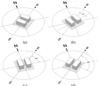
Next, 𝛼𝛼 values were classified into eight classes using equal intervals of 11.25 degrees, consistent with the angular range of cardinal points, and finally scored to represent the degree of airflow obstruction in the SW-NE direction (Table 1). Scores are based on an equal-interval scale and range between 12.5 (lowest) to 100 (highest). Figure 4 illustrates how 𝛼𝛼 values close to 90° indicate high potential of wind acceleration, while values near zero imply higher obstruction possibility for airflow.

𝜶𝜶 (degree) Score Degree of Wind _Obstruction _OrientationCanyon

[0–11.25] 100 Very high SE-NW

(11.25–22.50] 87.5

High ESE-WNW/ _SSE-NNW (22.50–33.75] 75 (33.75–45] 62.5 Medium E-W/ N-S (45–56.25] 50 (56.25–67.50] 37.5 _Low ENE-WSW/ NNE-SSW (67.50–78.75] 25

(78.75–90] 12.5 Very low NE-SW

Table 1. Allocated wind obstruction score based on the angle 𝛼𝛼 and the canyon orientations for the SW wind direction

Figure 4. Patterns of wind obstruction based on the angle 𝛼𝛼. (a) Maximum obstruction (α = 0°); (b) High obstruction (α ≈ 23°); (c) Medium obstruction (α ≈ 45°); (d) Channeling (α = 90°)

3.1.3. LCP analysis for mapping potential ventilation corridors. In 2010, Wong et al. introduced an original approach

to map high potential ventilation corridors across Hong Kong, based on the hypothesis that wind moves across the city following the path of lowest friction (Wong et al., 2010). In this approach, paths along which wind is least obstructed were identified using a surface roughness indicator and a LCP analysis. The LCP analysis is widely used in transportation planning to determine the most cost-effective path between two locations based on a cost distance determinant. While Wong et al. (2010) used FAI (at 100-m spatial resolution) as the cost determinant factor, we employed the allocated wind obstruction score raster map, based on canyon orientations (at 30-m spatial resolution), as the main cost distance determinant across the urban surface. Firstly, 73 starting and 71 ending points were created, where possible far from built structures, along equal distances (250 m) in the SW and NE boundaries of the study area, respectively. Then, a LCP from each of the 73 starting points to each of the 71 ending points was created using the Cost Distance and Cost Path tools in ArcMap 10.5, sequentially. The Cost Distance tool calculates at each pixel the least accumulative cost to the destination and identifies the backlink (i.e. the next pixel along the LCP), while the Cost Path tool draws the LCP. Finally, we have counted the number of times each pixel was passed by a LCP. This provides a measure of the frequency of occurrence of ventilation paths (Wong et al., 2010, p. 1882) in SW-NE direction. A GIS subroutine was designed using the visual The International Archives of the Photogrammetry, Remote Sensing and Spatial Information Sciences, Volume XLIII-B4-2020, 2020

(4)

programming language in ArcMap 10.5 for the automation of the entire procedure (see Appendix A).

3.1.4. In-situ measurements for method validation. In order

to validate the significance of the methodology for retrieving potential ventilation corridors across the city of Milan, a similar field observation to that conducted by Wong et al. (2010), was carried out to measure the maximum wind speed ū (m/s) along a path of relatively high ventilation. Field measurements were taken on July 30, 2018, when the average wind direction was forecasted to be in SW, according to the different weather stations close along the chosen path. During the site walk, 42 measurements were taken, where possible, along and off the path (i.e. in segments normal to the path) for the peak wind speed over a 2-minute time interval, using a digital portable anemometer that has a range of 0.50 to 30 m/s, 0.10 m/s resolution, and ±5% error accuracy. The filed measurements and the estimated frequency of occurrence at each pixel were averaged for each path segment in order to make direct comparisons.

3.2. Estimating the relative impact of ventilation corridors on maximizing the benefits of greening measures

The analysis in this section is based on the hypothesis that the cooling effect of urban green spaces can be improved if implemented along corridors of high ventilation. To test this assumption, different statistical tests have been employed. Firstly, a GWR model is used to model the spatial variation in the relationship between NDVI and near-surface air temperature. A GWR model is ideal for non-stationary spatial data (e.g. climate data), where for each location a local Ordinary Least Squares (OLS) regression equation is derived using all the observations falling within a certain bandwidth. Also, observations are weighted based on their distance from the regression point (Fotheringham et al., 1998). A GWR is written as:

𝑦𝑦𝑖𝑖= 𝛽𝛽0(𝑢𝑢𝑖𝑖, 𝑣𝑣𝑖𝑖) + � 𝛽𝛽𝑘𝑘 (𝑢𝑢𝑖𝑖, 𝑣𝑣𝑖𝑖)𝑥𝑥𝑖𝑖𝑘𝑘+ 𝜀𝜀𝑖𝑖 ,

𝑘𝑘 (3)

where at location 𝑖𝑖 defined by x-y coordinates (𝑢𝑢𝑖𝑖, 𝑣𝑣𝑖𝑖), 𝑦𝑦𝑖𝑖 is the dependent variable, 𝑥𝑥𝑖𝑖𝑘𝑘 are the independent variables, 𝛽𝛽𝑘𝑘 (𝑢𝑢𝑖𝑖, 𝑣𝑣𝑖𝑖) are the regression coefficients, 𝛽𝛽0(𝑢𝑢𝑖𝑖, 𝑣𝑣𝑖𝑖) is the intercept, and 𝜀𝜀𝑖𝑖 is the random error. In particular, we have defined two models for both daytime and night-time conditions using the GWR tool in ArcMap 10.5, where NDVI is the predictor and near-surface air temperature is the dependent variable. An optimal bandwidth was determined using the Akaike Information Criterion (AICc). As a next step, we have simulated the impact of equally increasing the NDVI values at each pixel along the retrieved paths on lowering the near-surface air temperature, using the local OLS regression equations. In particular, considering that the current maximum NDVI value identified is .78, we have increased NDVI values at each pixel by .22 (-1 ≤ NDVI ≤ 1). Afterwards, single ventilation corridors were defined as groups of adjacent pixels in a row that have similar occurrence frequency. The impact on lowering temperatures after increasing the NDVI values was estimated for each corridor for both daytime and night-time conditions.

However, since testing our hypothesis requires relying on accurate and precise predictions of temperature, based on simulated NDVI values (post intervention), and false negative results (i.e. temperature gains rather than losses) may affect the analysis, the local coefficient of determination (R2_{) here is of} great importance. Low R2 _{values indicate that the model has more}

error, while high values refer to better predictive performance. However, although, the overall adjusted R2 _{for the GWR} estimation can be very high, local R2 _{values may vary across the} area. Moreover, deciding what is a good R2_{value is controversial} and widely varies depending on the discipline and the study (Chin, 1998; Cohen, 1988; D. N. Moriasi et al., 2007; Hair, J. F., Hult, G. T. M., Ringle, C. M., & Sarstedt, 2013; Henseler et al., 2009). Nonetheless, in studies that examine the relationship between surface or near-surface air temperature and NDVI, local R2_{values higher than .50 are very common during the growing} season (Colaninno and Morello, 2019; Ferrelli et al., 2018; Guha et al., 2018); this depends on the vegetation type, the month, and the spatial resolution of the data. Hence, corridors with local R2 values lower than .50 may deem unsatisfactory for the purpose of this study and are excluded for the subsequent statistical analysis. Finally, in order to analyze the difference between the ventilation corridors in terms of their mean loss of temperature after the intervention (i.e. after increasing NDVI values), a hypothesis testing is used. Firstly, ventilation corridors were classified into three classes based on their average occurrence frequency, using the quantile method. This classification method is ideal for an ordinal classification of the ventilation corridors, where the total number of corridors in each class is approximately the same. Then, a one-way analysis of variance (ANOVA) was performed for both daytime and night-time. In particular, ANOVA compares the variance between three groups or more with the variance within groups to determine whether a significant difference exists between group means.

4. RESULTS AND ASSESSMENT 4.1. Spatial distribution of urban ventilation corridors

A total of 5183 LCPs were created across the city of Milan, which together resulted in around 445 single ventilation corridors. The spatial distribution of the ventilation corridors (Figure 5) shows that high potential ventilation areas are mostly located in the central and northern parts of the city compared to the southern parts which have relatively less ventilation. In particular, five major paths were recognized to have the highest potential of ventilation in the northern part of the city and which connect the major regional outer parks; these are (ABCDEFG), (CHIJE), (KLMNOP), (STL), and (OQR).

The in-situ measurements along path (ABCDEFG) showed that, in general, the mean maximum wind speeds recorded off the path segments are much lower than the mean maximum wind speeds along the same segments. For instance, mean maximum wind speeds of 2.50 m/s and 0.60 m/s were recorded along and off segment EF, respectively. The same was observed for segments CD (2.27 m/s vs. 1.60 m/s) and DE (2.20 m/s vs. 0.65 m/s). Also, relatively higher wind speeds were observed to be along segments of higher occurrence frequency. For example, a mean maximum wind speed of 2.50 m/s was recorded along segment EF with the highest modelled average occurrence frequency of 1155, while for segments CD and DE, along which average occurrence frequencies are 782 and 569, maximum wind speeds are 2.27 m/s and 2.18 m/s, respectively. This slight decrease in the measured wind speeds from segment EF to CD and from segment CD to DE is congruent with the differences in their average occurrence frequencies. Despite the measurement uncertainty, due to the relatively low accuracy of the anemometer used (±5%), the differences found between the measurements along and off the path can still justify the relevance of the proposed method to identify potential ventilation corridors at large scale.

(5)

Figure 5. Retrieved ventilation corridors in SW-NE direction and occurrence frequency, using canyon orientations and LCP analysis

4.2. Impact of ventilation corridors on the cooling effect of greening solutions

4.2.1. GWR model diagnostics and temperature simulations. Statistical summary of the GWR models is given in

Table 2. The adjusted R2_{was estimated to be .970 and .955 for} daytime and night-time conditions, respectively.

GWR Parameters _{(10:30 AM)}Daytime _{(09:30 PM)}Night-time Observations (N) 8788 8788

Bandwidth (m) 289.637647 289.637647

Sigma 0.114432 0.265130

R2 _.973531 _.960272

R2_adj. _.970210 _.955287

Table 2. GWR model parameters for both daytime and night-time, where Sigma is the square root of the normalized residual

sum of squares. R2_{is the coefficient of determination, and R}2 adj. is the adjusted coefficient of determination Furthermore, Table 3 shows the ordinal classification of the ventilation corridors after excluding corridors with relatively low local R2_{(< .50) as outlined in}_{section 3.2}_.

In particular, from a total of 445 corridors, 44 and 64 were excluded for daytime and night-time, respectively. Also, the mean difference in near-surface air temperature (∆ 𝑇𝑇) after increasing NDVI values, is reported for each class in Table 3. As expected, an increase in NDVI values has generally reduced the average near-surface air temperature. Locally, the impact of vegetation on lowering temperature is more significant, especially at night-time. Figure 6 shows an example of current and simulated values for NDVI and near-surface air temperature along segment EF.

Daytime (10:30 AM)

Class Occurrence Frequency n ∆ 𝑇𝑇 (°C)

A 1569–307 High 132 0.657061705

B 306–115 Medium 136 0.679894279

C 114–4 Low 133 0.656986594

Night-time (09:30 PM)

Class Occurrence Frequency n ∆ 𝑇𝑇 (°C)

A 1569–272 High 127 1.086904685

B 271–104 Medium 127 1.087278969

C 103–4 Low 127 0.967112126

Table 3. Ordinal classification of the ventilation corridors and the mean loss in temperature (°C) by class

(6)

Figure 6. Current and simulated NDVI and near-surface air temperature along segment EF for daytime (top) and night-time

(bottom)

4.2.2. Differences among ventilation corridors in lowering near-surface air temperature. Regarding the ∆ 𝑇𝑇 variation

among green corridors with different degree of ventilation, the results from the one-way ANOVA are presented in Table 4. Daytime (10:30 AM) SS Df MS F p Between Groups 0.047 2 0.024 1.199 .303 Within Groups 7.802 398 0.020 Total 7.849 400 Night-time (09:30 PM) SS Df MS F p Between Groups 1.219 2 0.609 5.244 .006 Within Groups 43.927 378 0.116 Total 45.146 380

Table 4. ANOVA summary for daytime and night-time, where SS is the sum of squares, df is the degree of freedom, MS is the mean square, F is the F-statistics, and p is the probability value In particular, results show that at night, we can reject the null hypothesis, and that the three classes of ventilation corridors

differ significantly in their mean loss of temperature (p < .05). However, during daytime, there is not any significant difference between classes (p > .05). This indicates that urban green ventilation corridors are more effective during night-time when the UHI effect is peaked. This can be explained as green spaces have generally low heat capacity and thus cool off faster at night. However, an ANOVA can tell us whether there is a significant difference between classes or not, but it does not tell where these differences exactly happen. Hence, we used a Post-Hoc analysis after an ANOVA to compare each pair of the class means for the night-time condition. In particular, we used the Tukey’s Honest Significant Difference test (Tukey HSD) followed by Cohen’s d to calculate the effect size for the differences in pairwise (Figure 7 and Table 5). Cohen’s d is a measure of effect size which quantifies the magnitude of the difference between groups. It is calculated by dividing the mean difference of two groups by their pooled standard deviation (Cohen, 1988). While there was no significant difference between class A and class B (p > .05), both yielded significantly lower results when compared to class C (p < .05). Cohen’s d effect size indicates that the two statistically significant pairs, i.e. A-C and B-C have effect sizes of 0.35 and 0.37, respectively, which are considered of small-to-medium magnitude (Cohen, 1988). This can be returned to the average low wind speed recorded for the day of the analysis (≈ 1.5 m/s). However, this demonstrates that even under very calm wind conditions, there is still an opportunity for increasing, even if just a little bit, the benefits of greening measures in terms of lowering high temperatures in cities.

Figure 7. The mean loss in night-time temperature (°C) for each class of ventilation corridors. Bars represent standard deviation

and asterisks indicate significant differences between classes

* The mean difference is significant at the .05 level

Table 5. Tukey's multiple comparisons test and Cohen’s d effect size

5. DISCUSSION AND CONCLUSION

In this paper, we have discussed the development of a complete methodology for identifying potential urban ventilation corridors and subsequently assessing their relative impact on maximizing the benefits of urban green solutions, as some of the most used UHI mitigation measures in cities.

In the first part, canyon orientations were calculated using Euclidean geometry. Then, around 445 corridors were delineated in SW-NE direction across the city of Milan, using a LCP

analysis. The relative difference in ventilation between the identified corridors was found to be relevant when compared against in-situ measurements of maximum wind speeds. However, this approach is suitable for the normal case, i.e. for cities of uniform urban structure in terms of average building heights, intermediate aspect ratios, and elongated canyons; otherwise, other parameters should be included to better model airflow patterns in cities (e.g. height-to-width ratio of street canyons, building roofs geometry; Oke et al., 2017). In general, in order to accurately model ventilation across cities, a 3D approach should be considered, whereby 2D and 3D roughness

Tukey HSD test Mean Diff. 95.00% CI of diff. Significant? Summary Adjusted P value Cohen’s d

Class A vs. Class B -0.0003743 -0.1010 to 0.1003 No ns > .9999 0.001041

Class A vs. Class C 0.1198 0.01913 to 0.2205 Yes * .0148 0.351752

Class B vs. Class C 0.1202 0.01951 to 0.2208 Yes * .0144 0.373272

(7)

attributes are employed. Higher quality elevation models (e.g. LIDAR-derived digital surface models) can be utilized for this purpose.

In the second part, we have assessed whether the impact of green solutions upon lowering temperature can be maximized if incremented along corridors of relatively high ventilation. For this purpose, firstly, a GWR model, where NDVI is the predictor and near-surface air temperature is the dependent variable, was defined for both daytime and night-time conditions, to simulate the impact on lowering temperature after equally increasing green intensity. Then, ventilation corridors were assessed for statistical significance of difference in near-surface air temperature before and after the intervention. Results from the one-way analysis of variance (ANOVA) showed that the effect of green ventilation corridors is more significant at night, which is adequate for mitigating the UHI effect that is most developed at this time. Also, it has been demonstrated that even under very calm wind conditions, there is still an opportunity for maximizing the benefits of greening measures in terms of lowering high temperature. This research finding is very promising, especially for cities where wind is a marginal potentiality like Milan. This work highlights only an example of the promising role of urban computation, employing digital mapping, spatial analysis, and statistical modelling, in supporting urban climate design and planning for combating climate change.

REFERENCES

Belcher, S.E., 2005. Mixing and transport in urban areas. Philos Trans R Soc A Math Phys Eng Sci. https://doi.org/10.1098/rsta.2005.1673

Bernard, J., Rodler, A., Morille, B., Zhang, X., 2018. How to design a park and its surrounding urban morphology to optimize the spreading of cool air? Climate. https://doi.org/10.3390/cli6010010

Burian, S.J., Velugubantla, S.P., Brown, M.J., 2002. Morphological Analyses using 3D Building Databases: Phoenix, Arizona. La-Ur-01-4055.

Chang, S., Jiang, Q., Zhao, Y., 2018. Integrating CFD and GIS into the development of urban ventilation corridors: A case study in Changchun City, China. Sustain. https://doi.org/10.3390/su10061814

Chen, S.L., Lu, J., Yu, W.W., 2017. A quantitative method to detect the ventilation paths in a mountainous urban city for urban planning: A case study in guizhou, China. Indoor Built Environ. https://doi.org/10.1177/1420326X15626233

Chin, W.W., 1998. The partial least squares approach for structural equation modeling., in: Modern Methods for Business Research.

Cohen, J., 1988. Statistical power analysis for the behavioral sciences (2nd ed.). Hillsdale, NJ: Lawrence Earlbaum Associates., Lawrence Earlbaum Associates.

Colaninno, N., Morello, E., 2019. Modelling the impact of green solutions upon the urban heat island phenomenon by means of satellite data, in: Journal of Physics: Conference Series. https://doi.org/10.1088/1742-6596/1343/1/012010

Counihan, J., 1975. Adiabatic atmospheric boundary layers: A

review and analysis of data from the period 1880-1972. Atmos Environ. https://doi.org/10.1016/0004-6981(75)90088-8 D. N. Moriasi, J. G. Arnold, M. W. Van Liew, R. L. Bingner, R. D. Harmel, T. L. Veith, 2007. Model Evaluation Guidelines for Systematic Quantification of Accuracy in Watershed

Simulations. Trans ASABE. https://doi.org/10.13031/2013.23153

Esri Inc., 2016. ArcMap 10.5 [Computer software].

Fabrizi, R., Bonafoni, S., Biondi, R., 2010. Satellite and ground-based sensors for the Urban Heat Island analysis in the city of Rome. Remote Sens. https://doi.org/10.3390/rs2051400

Ferrelli, F., Huamantinco Cisneros, M.A., Delgado, A.L., Piccolo, M.C., 2018. Spatial and temporal analysis of the LST-NDVI relationship for the study of land cover changes and their contribution to urban planning in monte hermoso, Argentina. Doc d’Analisi Geogr. https://doi.org/10.5565/rev/dag.355 Fotheringham, A.S., Charlton, M.E., Brunsdon, C., 1998. Geographically weighted regression: a natural evolution of the expansion method for spatial data analysis. Environ Plan A. https://doi.org/10.1068/a301905

Gál, T., Lindberg, F., Unger, J., 2009. Computing continuous sky view factors using 3D urban raster and vector databases: Comparison and application to urban climate. Theor Appl Climatol. https://doi.org/10.1007/s00704-007-0362-9

Gál, T., Unger, J., 2009. Detection of ventilation paths using high-resolution roughness parameter mapping in a large urban area. Build Environ. https://doi.org/10.1016/j.buildenv.2008.02.008

Grimmond, C.S.B., Oke, T.R., 1999. Aerodynamic properties of urban areas derived from analysis of surface form. J Appl Meteorol. https://doi.org/10.1175/1520-0450(1999)038<1262:APOUAD>2.0.CO;2

Guha, S., Govil, H., Dey, A., Gill, N., 2018. Analytical study of land surface temperature with NDVI and NDBI using Landsat 8 OLI and TIRS data in Florence and Naples city, Italy. Eur J Remote Sens. https://doi.org/10.1080/22797254.2018.1474494 Hair, J. F., Hult, G. T. M., Ringle, C. M., & Sarstedt, M., 2013. A Primer on Partial Least Squares Structural Equation Modeling (PLS-SEM). Thousand Oaks. Sage.

Henseler, J., Ringle, C.M., Sinkovics, R.R., 2009. The use of partial least squares path modeling in international marketing. Adv Int Mark. https://doi.org/10.1108/S1474-7979(2009)0000020014

Hsieh, C.M., Huang, H.C., 2016. Mitigating urban heat islands: A method to identify potential wind corridor for cooling and ventilation. Comput Environ Urban Syst. https://doi.org/10.1016/j.compenvurbsys.2016.02.005

Kropf, K., 1996. Urban tissue and the character of towns. Urban Des Int. https://doi.org/10.1057/udi.1996.32

Lettau, H., 1969. Note on Aerodynamic Roughness-Parameter Estimation on the Basis of Roughness-Element Description. J Appl Meteorol. https://doi.org/10.1175/1520-0450(1969)008<0828:noarpe>2.0.co;2

(8)

Ninyerola, M., Pons, X., Roure, J.M., 2000. A methodological approach of climatological modelling of air temperature and precipitation through GIS techniques. Int J Climatol.

https://doi.org/10.1002/1097-0088(20001130)20:14<1823::AID-JOC566>3.0.CO;2-B NOAA, 2018. Global Climate Report - Annual 2017. Natl Centers Environ Inf.

Oke, T.R., Mills, G., Christen, A., Voogt, J.A., 2017. Urban Climates. Cambridge University Press, Cambridge. https://doi.org/10.1017/9781139016476

Rasul, A., Balzter, H., Smith, C., Remedios, J., Adamu, B., Sobrino, J., Srivanit, M., Weng, Q., 2017. A Review on Remote Sensing of Urban Heat and Cool Islands. Land. https://doi.org/10.3390/land6020038

Ren, C., Yang, R., Cheng, C., Xing, P., Fang, X., Zhang, S., Wang, H., Shi, Y., Zhang, X., Kwok, Y.T., Ng, E., 2018. Creating breathing cities by adopting urban ventilation assessment and wind corridor plan – The implementation in Chinese cities. J

Wind Eng Ind Aerodyn. https://doi.org/10.1016/j.jweia.2018.09.023

Rouse, J.W., Hass, R.H., Schell, J.A., Deering, D.W., Harlan, J.C., 1974. Monitoring the vernal advancement and retrogradation (green wave effect) of natural vegetation. Final Report, RSC 1978-4, Texas A M Univ Coll Station Texas. Ruefenacht, L., Acero, J.A., 2017. Strategies for Cooling Singapore. https://doi.org/10.3929/ETHZ-B-000258216

Samsonov, T.E., Konstantinov, P.I., Varentsov, M.I., 2015. Object-oriented approach to urban canyon analysis and its applications in meteorological modeling. Urban Clim. https://doi.org/10.1016/j.uclim.2015.07.007

Spirn, A., 1987. Better air quality at street level: strategies for urban design. Public streets public use Van Nostrand Reinhold, ….

Suder, A., Szymanowski, M., 2014. Determination of Ventilation Channels In Urban Area: A Case Study of Wrocław (Poland). Pure Appl Geophys. https://doi.org/10.1007/s00024-013-0659-9 Voogt, J.A., Oke, T.R., 1997. Complete urban surface temperatures. J Appl Meteorol. https://doi.org/10.1175/1520-0450(1997)036<1117:CUST>2.0.CO;2

Weng, Q., Lu, D., Schubring, J., 2004. Estimation of land surface temperature-vegetation abundance relationship for urban heat island studies. Remote Sens Environ. https://doi.org/10.1016/j.rse.2003.11.005

Wicht, M., Wicht, A., Osińska-Skotak, K., 2017. Detection of ventilation corridors using a spatio-temporal approach aided by remote sensing data. Eur J Remote Sens. https://doi.org/10.1080/22797254.2017.1318672

Wong, M.S., Nichol, J.E., To, P.H., Wang, J., 2010. A simple method for designation of urban ventilation corridors and its application to urban heat island analysis. Build Environ. https://doi.org/10.1016/j.buildenv.2010.02.019

Xu, Y., Qin, Z., Shen, Y., 2012. Study on the estimation of near-surface air temperature from MODIS data by statistical methods.

Int J Remote Sens. https://doi.org/10.1080/01431161.2012.701351

Yan, H., Zhang, J., Hou, Y., He, Y., 2009. Estimation of air temperature from MODIS data in east China. Int J Remote Sens. https://doi.org/10.1080/01431160902842375

Zhang, M., Bae, W., Kim, J., 2019. The effects of the layouts of vegetation and wind flow in an apartment housing complex to mitigate outdoor microclimate air temperature. Sustain. https://doi.org/10.3390/su11113081

Zhao, C., Jensen, J., Weng, Q., Weaver, R., 2018. A geographically weighted regression analysis of the underlying factors related to the surface Urban Heat Island Phenomenon. Remote Sens. https://doi.org/10.3390/rs10091428

Zhao, L., Lee, X., Smith, R.B., Oleson, K., 2014. Strong contributions of local background climate to urban heat islands. Nature. https://doi.org/10.1038/nature13462

APPENDIX

Appendix A. Model workflow to elaborate Least Cost Paths (LCPs) from starting points, ending points, and a cost surface in

ArcMap 10.5