Neural network architectures for information extraction from hyper-spectral images

(1)

Universit`a degli Studi di Roma “Tor Vergata”

Facolt`

a di Ingegneria

Ph.D Geoinformation Programme

XXII Cycle

Neural network architectures for

information extraction from

hyper-spectral images

Geoinformation Ph.D Thesis

Tutor Candidate

Fabio Del Frate Giorgio Antonino Licciardi

(2)

(3)

5 Production of land cover maps from multi-temporal and multi-angular hyper-spectral data 83 5.1 Introduction . . . 83 5.2 Multi-temporal dataset . . . 84 5.2.1 Feature extraction . . . 85 5.2.2 Classification . . . 87 5.3 Multi-angular/temporal dataset . . . 91 5.3.1 Feature extraction . . . 92 5.3.2 Classification . . . 92 5.4 Spectral unmixing . . . 95 5.5 Conclusions . . . 109

6 Urban area classification using high resolution hyperspec-tral data 111 6.1 Introduction . . . 111

6.2 Majority voting between NN and ML classifiers . . . 114

6.2.1 Dimensionality reduction . . . 114

(5)

CONTENTS v 6.3 NLPCA approach . . . 117 6.3.1 Dimensionality reduction . . . 117 6.4 Classification . . . 120 6.5 Conclusions . . . 120 Conclusions 125 Bibliography 146

(6)

(7)

Abstract

Imaging spectroscopy, also known as hyper-spectral remote sensing, is an imaging technique capable of identifying materials and objects in the air, land and water on the basis of the unique reflectance patterns that result from the interaction of solar energy with the molecular structure of the material. Recent advances in aerospace sensor technology have led to the development of instruments capable of collecting hundreds of images, with each image corresponding to narrow contiguous wavelength intervals, for the same area on the surface of the Earth. As a result, each pixel (vector) in the scene has an associated spectral signature or “fingerprint” that uniquely characterizes the underlying objects.

Hyper-spectral sensors mainly cover wavelengths from the visible range (0.4µm- 0.7µm) to the middle infrared range (2.4µm). If we consider the consistency of this data, we can easily understand the importance of finding a method which can transform the data cube into one with reduced dimen-sionality and maintain, at the same time, as much information content as possible. These techniques are known under the general name of feature reduction. Besides enabling an easier storage and management of the data, features reduction procedures can be crucial for the implementation of

(8)

op-timum inversion algorithms.

This research work strives to give a contribution along the direction of extracting information from hyperspectral data. A major instrument is considered for this purpose, which is the use of neural networks algorithms, already recognized to represent a rather competitive family of algorithms for the analysis of hyperspectral data. Besides introducing a novel neural network approach for handling the dimensionality reduction of hyperspec-tral data, other specific issues will be considered, with a special focus on the unmixing problem, or sub-pixel classification.

While the first three chapters are dedicated to the presentation of the problems, to the current state of art and to the, theoretically sound, pro-posed solutions, the remaining sections are dedicated to the description and the assessment of the results obtained in different applicative scenar-ios. Some final considerations conclude the work.

(9)

Chapter 1

Hyper-spectral data

Both scientists and common people are becoming increasingly concerned with environmental phenomena such as the photosynthetic conditions of the vegetation, wide deforestation and fires, desertification, sea pollution, together with the general health of the Earth. The monitoring of these events and the understanding of the impact which they could have on the fragile biophysical mechanisms is becoming more and more important than in the past. For this reason, sensors like MERIS, MODIS, AVHRR and AATSR have been designed and placed in orbit. These measurements are performed using several spectral bands (up to 36 for MODIS) located into the visible and the infrared range in order to collect a noteworthy dataset for every kind of global investigation (land use, ocean color, snow cover, sea ice observation...). A following step has been the allocation of many contiguous and narrow bands (more than one hundred) available for the measurement. This technological evolution led to the hyper-spectral im-agery, which has demonstrated very high performance in several cases of

(10)

Figure 1.1: Hyper-cube obtained from a AVIRIS dataset

material identification and urban mapping, including sub pixel classifica-tion. The hyper-spectral sensors differ from each other in terms of number of bands, bandwidth, spatial resolution and spectral range, spatial acquisi-tion and spectral selecacquisi-tion modes. Managing such dissimilar type of data is not a simple task and requires the adoption of information extraction techniques that are appropriate for each specific sensor data.

1.1 Data acquisition principles

In general, hyper-spectral sensors can be divided into three different scan-ning systems for acquiring the image:

(11)

1.1 Data acquisition principles 5 telescopes with scan mirrors sweep from one edge of the swath to the other. The Field of View (FOV) of the scanner can be detected by a single detector or a single-line-detector. This means that the dwell time for each ground cell must be very short at a given Instantaneous Field of View (IFOV), because each scan line consists of multiple ground cells which will be detected.

• Pushbroom scanners: as electronic scanners they use a detector array to scan over a two dimensional scene. The number of across track pixels detector pixel is equal to the number of ground cells for a given swath. The motion of the aircraft or spacecraft provides the scan in along-track-direction. Pushbroom scanners are the standard for high resolution imaging spectrometers.

• Staring imagers: these imagers are also electronic scanners. They detect a two dimensional FOV at once. The IFOV along and cross track corresponds to the two dimensions of detector area array. Two sub-groups of staring imagers are Wedge Imaging Spectrometer (WIS) and Time Delay Integration Imager (TDI).

Hyper-spectral spectrometers can also have very different spectral se-lection modes:

Dispersion elements (grating, prism): This group collects spectral images by using a grating or a prism. The incoming electromagnetic ra-diation will be separated into different angles. The spectrum of a single ground pixel will be dispersed and focused at different locations of one di-mension of the detector array. This technique is used for both whiskbroom

(12)

Figure 1.2: Scanning approaches

(13)

1.1 Data acquisition principles 7 and pushbroom image acquisition modes. Most hyper-spectral imagers are using grating as dispersive elements, whereas some use prisms.

Filter based systems: a narrow band of a spectrum can be selected by applying optical bandpass filters (tunable filters, discrete filters and linear wedge filters). A linear wedge transmits light at a centre wavelength that depends on the spatial position of the illumination in the spectral dimen-sion. The detector behind the device receives light at different wavelengths of the scene.

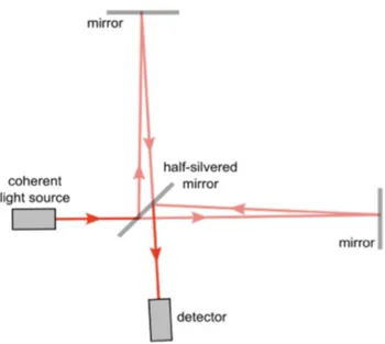
Fourier-Transform Spectrometers (FTS): a Fourier-transform spec-trometer is an adaption of the Michelson interferometer [1] where a colli-mated beam from a light source is divided into two by a beamsplitter and sent to two mirrors. These mirrors reflect the beams back along the same paths to the beamsplitter, where they interfere. The signal recorded at the output depends on the wavelength of the light and the optical path differ-ence between the beamsplitter and each of the two mirrors. If the optical path difference between the two beams is zero or a multiple of the wave-length of the light then the output will be bright, otherwise if the optical path difference is an odd multiple of half the wavelength of the light then the output will be dark.

In the Fourier transform spectrometer, one of the mirrors is scanned in the direction parallel to the light beam. This changes the path difference between the two arms of the interferometer, hence the output alternates between bright and dark fringes. If the light source is monochromatic, then the signal recorded at the output will be modulated by a cosine wave; if it is not monochromatic then the output signal will be the Fourier transform

(14)

Figure 1.4: Schematic of a Fourier-Transform Spectrometer

of the spectrum of the input beam. The spectrum can then be recovered by performing an inverse Fourier-transform of the output signal.

1.2 Data uniformity

Efficient and accurate imaging spectroscopy data processing asks for per-fectly uniform data in both spectral and spatial dimensions. The precision of a measurement is determined by the instrument response r(z), with z the position coordinate. The transformation from the input physical quantity to the measurement O(z) is described mathematically by a convolution:

O(z0) =

Z

W

(15)

1.2 Data uniformity 9 Or in shorthand notation:

O(z) = i(z) ⊗ r(z) (1.2) Where:

i(z): input signal

r(z − z0): sensor response at the position z0

O(z0): output signal, assigned to the position z = z0

W : significant spatial range covered by the response of the system. The image of a scene viewed by the sensor is not completely its faithful reproduction. Small details are blurred relative to larger features; this blurring is characterized by the total sensor Point Spread Function (PSF). The response of a detector element depends principally from the PSF, which can be viewed as the spectral/spatial responsivity of the sensor.

PSF consists of several components:

• Optical PSF (P SFopt), defined by the spatial energy distribution in

the image of a point source. Being an optical system not perfect, the energy from a point source is spread over a small area in the focal plane. The extent of spreading depends on many factors, including optical diffraction, aberrations, and mechanical assembly quality. • The image motion PSF (P SFIM), caused by the motion of the

car-rier during the integration time, which lead normally to rectangular spatial pixel response shapes.

• The detector PSF (P SF_det) produces a spatial blurring caused by the non-zero spatial area of each detector in the sensor, and also normally

(16)

is not a quadratic shape.

• The electronics PSF (P SF_el), appearing by electronic filtering of the acquired data during acquisition, e.g. for correction of dark current or smear effects.

From these four influences, the total PFS can be expressed by a combination of these effects:

P SF = P SFopt+ P SFIM+ P SFdet+ P SFel (1.3)

For pushbroom imaging spectroscopy, one image frame registers the spectral and spatial dimension simultaneously. Any non-uniformity in the system generates degrading artifacts, more in particular:

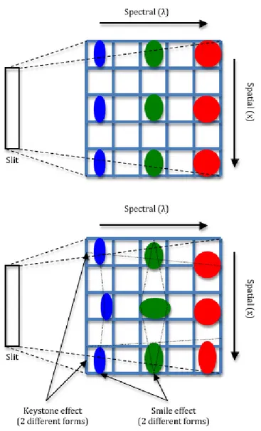
• Spectral PSF non-uniformity: is the non-uniformity of the spectral response within a sensor’s spectral band and can be imaged on a detector row as shown in fig.1.5. This non-uniformity is typically represented by the position and shape of the spectral response func-tion. The related artifacts of spectral misregistration are denoted as “smile” or “frown”.

• Spatial PSF non-uniformity: is the non-uniformity of the spatial re-sponse within an acquired spectrum and is usually imaged on a de-tector column as shown in fig.1.5. This non-uniformity is represented by the position and shape of the spatial response function in both the along-track and across-track dimensions of a spatial pixel. The related artifacts in the across-track dimension are denoted as “keystone”.

(17)

1.2 Data uniformity 11 As for the spatial non-uniformity, the influence of the “keystone” effect results in a black pixel in the image that can be easily replaced. On the other hand the removal of the “smile” effect is not an easy task.

1.2.1 Influence of smile effect on pushbroom sensor

In many cases a pushbroom sensor can be affected by the “smile effect” [2]. The consequence of this effect is that the central wavelength of a band varies with spatial position across the width of the image in a smoothly curving pattern fig.1.6. Very often the peak of the smooth curve tends to be in the middle of the image and give it a shape of “smile” or “frown”. That is why this spectral misalignment is termed as smile effect. The effect of the smile is not obvious in the individual bands. Therefore an indicator is needed to make evident whether or not a given image suffers from smile effect. A way to check for the smile effect is to look at the band around atmospheric absorption (760 nm)[reference smile]different images. In fact, the region of red-near infrared transition has high information content of vegetation spectra. This region is generally called “red-edge” (670-780 nm) and identifies the red-edge position (REP) [3] [4]. REP is a good indica-tor of chlorophyll concentration. Increase in amount of vegetation causes shift in red-edge slope and REP towards longer wavelengths. In contrast, low chlorophyll concentration causes shift in red-edge slope towards shorter wavelengths. The smile effect is acute due to sharp absorption at 760 nm, which is within the red-edge region, and for this reason atmospheric correc-tion of smiled data will be incorrect. Although some research has been done on many hyper-spectral datasets to solve the smile problem, the researchers

(18)

Figure 1.5: PSF in ideal (top) and real (bottom) position: the smile and keystone effects on a detector

(19)

1.2 Data uniformity 13

Figure 1.6: Smooth curves representing the spectral variations along the spatial domain. Frown (top) and smile effect (bottom)

(20)

have yet not come up with a complete solution. The methodologies devel-oped so far can only reduce the intensity of smile effect but cannot remove it entirely, because during its life a detector element can change its response, therefore the knowledge and the correction of this phenomena became fun-damental in the analysis of hyper-spectral images and more in general in multispectral images.

In the following paragraph I will list the main hyper-spectral sensors, and describe in details their main features, peculiarities and usage (employ-ment, applications, etc).

1.3 Airborne Hyper-spectral sensors

The latest airborne payloads include sensors with measurements carried out at thousands of wavelengths and at the finest spatial resolution.

1.3.1 CASI

The Compact Airborne Spectrographic Imager (CASI) [5], produced by Itres Research of Canada, is a two-dimensional Charge-Coupled-Device (CCD) array based pushbroom imaging spectrograph.

One dimension of the 578x288 element array is used to obtain a 512 spatial pixels frame of the surface that builds up a flightline of data as the aircraft moves forward. The front side of the CASI camera head is equipped with a custom fore-optic lens with 54.4◦FOV which has been designed to provide optimum focusing across the CASI wavelength range (achromatic focus).

(21)

1.3 Airborne Hyper-spectral sensors 15

Parameter Description IFOV 40◦

Spectral Range 650nm between 380 and 1050nm Spatial Samples 512 pixels

Bands 288 Bandwidth < 3.5 nm Dynamic Range 14 bits

Table 1.1: CASI spectral parameters

(22)

grating disperses the light from each pixel over the 405nm to 950nm spectral range and is recorded by the 288 detectors on the orthogonal dimension of the CCD. The row spacing on the CCD equates with a spectral sampling of 1.8nm. The effective bandwidth of a single row has an approximate value of 2.2 nm FWHM (Full Width at only Half its Maximum value) at 650nm, resulting from the optical system and convolution of the slit width and detector size.

1.3.2 AHS

The Airborne Hyper-spectral Scanner (AHS) [6] is an 80-bands airborne imaging radiometer, developed by ArgonST (USA) and operating by INTA. It has 63 bands in the reflective part of the electromagnetic spectrum, 7 bands in the 3 to 5 microns range and 10 bands in the 8 to 13 microns region. The first element of the system is a rotating mirror, which directs the surface radiation to a cassegrain-type telescope. The telescope design includes a so-called pfund-assembly, that defines a 2.5 mrad IFOV and acts as a field stop. This field is therefore unique for all bands, and redirects the radiation to a spectrometer placed above the telescope. In the spectrometer, four dichroic filters are used to split the incoming radiation in five optical ports: Port 1 (corresponding to VNIR wavelengths), Port 2a (for a single band at 1.6 micrometers), Port 2 (SWIR), Port 3 (MIR) and Port 4 (TIR). For each of the ports, a grating disperses the radiation and a secondary optical assembly focuses it onto an array of detectors, which defines the final set of (contiguous) spectral bands. Table 1.2 displays the resulting spectral configuration.

(23)

1.3 Airborne Hyper-spectral sensors 17

Parameter Description IFOV 2.5 mrad Spectral Ranges

VIS/NIR (Port 1) 441-1018nm NIR (Port 2A) 1.491-1.650 µm NIR (Port 2) 2.019-2.448 µm MIR (Port 3) 3.03-5.41 µm LWIR (Port 4) 7.950-13.17 µm Spatial Samples 750 pixels Bands 80

Bandwidths

VIS/NIR (Port 1) 30 nm NIR (Port 2A) 0.2 µm NIR (Port 2) 0.013 µm MIR (Port 3) 0.3 µm LWIR (Port 4) 0.4-0.5 µm Dynamic Range 12 bits

(24)

Figure 1.8: MIVIS (left) and AHS (right) Hyper-spectral Imagers

1.3.3 MIVIS

MIVIS [7] (Multispectral Infrared and Visible Imaging Spectrometer) is a modular hyper-spectral scanner composed of 4 spectrometers, which si-multaneously measure the electromagnetic radiation of the Earth’s surface recorded by 102 spectral bands. The instrument can be considered as one of the imaging spectrometers of second generation, that best meets the research needs because it enables advanced applications in environmental remote sensing, like Agronomy, Archaeology, Botanic, Geology, Hydrology, Oceanography, Pedology, Urban Planning, Atmospheric Sciences, and so on.

The simultaneous scanning in a great number of channels with a high spectral and spatial resolution require the highly technological optics and sensors, electronic pre-processing and registration of a large data quantity. The combination of a high resolution in the Mid Infrared region with a good sensitivity in the Thermal Infrared region has caused many problems during the design phase. The resulting system is a mechanical scanning

(25)

1.3 Airborne Hyper-spectral sensors 19 Parameter Description IFOV 2.0 mrad Spectral Ranges VIS 0.43-0.83 µm NIR 1.15-1.55 µm MIR 2.0-2.5 µm TIR 8.2-12.7 µm Spatial Samples 755 pixels Bands 102 Bandwidths VIS 0.02 µm NIR 0.05 µm MIR 0.009 µm TIR 0.34-0.54 µm Dynamic Range 12 bits

Table 1.3: MIVIS spectral parameters

optical instrument provided with a sensor for each spectral region that collects energy from a common Field Stop for all channels.

1.3.4 AVIRIS

AVIRIS (Airborne Visible InfraRed Imaging Spectrometer) is a premier in-strument in the realm of Earth Remote Sensing developed by NASA [8]. AVIRIS contains 224 different detectors, each with a bandwidth of approxi-mately 10 nanometers, allowing it to cover the entire range between 380 nm and 2500 nm. AVIRIS uses a whiskbroom scanning mirror producing 677 pixels for the 224 detectors at each scan. The pixel size and swath width of the AVIRIS data depend on the altitude from which the data is collected.

(26)

Parameter Description IFOV 1.0 mrad Spectral Ranges 380-2500 nm Spatial Samples 677 pixels Bands 224 Bandwidths 10 nm Dynamic Range 12 bits

Table 1.4: AVIRIS spectral parameters

The ground data is recorded on board the instrument along with navigation and engineering data and the readings from the AVIRIS on-board calibra-tor. When all of this data is processed and stored on the ground, it yields approximately 140 Megabytes (MB) for every 512 scans (or lines) of data. Each 512 line set of data is called a ”scene”, and corresponds to an area about 10km long on the ground. Every time AVIRIS flies, the instrument takes several runs of data (also known as flight lines). A full AVIRIS disk can yield about 76 Gigabytes (GB) of data per day.

1.3.5 ROSIS

ROSIS (Reflective Optics System Imaging Spectrometer) [9], a compact airborne imaging spectrometer, developed jointly by MBB Ottobrunn (now EADS-ASTRIUM), GKSS Geesthacht (Institute of Hydrophysics) and DLR Oberpfaffenhofen (former Institute of Optoelectronics) based on an origi-nal design for a flight on ESA’s EURECA platform. The design driver for ROSIS was its application for the detection of spectral fine structures espe-cially in coastal waters. This task determined the selection of the spectral range, bandwidth, number of channels, radiometric resolution and its tilt

(27)

1.4 Satellite Hyper-spectral sensors 21

Figure 1.9: AVIRIS hyper-spectral Imager Parameter Description IFOV 0.56 mrad Spectral Ranges 430-860 nm Spatial Samples 512 pixels Bands 115 Bandwidths 4.0 nm Dynamic Range 14 bits

Table 1.5: ROSIS spectral parameters

capability for sun glint avoidance. However, ROSIS can be exploited for monitoring spectral features above land or within the atmosphere.

1.4 Satellite Hyper-spectral sensors

The development of hyper-spectral technology for the space satellites re-mains difficult and very expensive in terms of payload design, maintenance and calibration. However, these difficulties have not deterred the space

(28)

Figure 1.10: ROSIS instrument

agencies from finding interesting missions carrying on board hyper-spectral payloads. This is the case of Hyperion developed by NASA, CHRIS Proba-1 developed by a European consortium founded by ESA, and the upcoming PRISMA developed by ASI (Agenzia Spaziale Italiana), and EnMAP de-veloped by DLR.

1.4.1 HYPERION

Hyperion instrument [10], mounted onboard of the National Aeronautics and Space administration (NASA) EO-1 satellite, provides a high resolu-tion hyper-spectral imager capable of resolving 220 spectral bands (from 0.4 to 2.5 µm) with a 30 meter spatial resolution. The instrument covers a 7.5 km by 100 km land area per image and provides detailed spectral mapping across all 220 channels with high radiometric accuracy. The ma-jor components of the instrument are the System fore-optics design based

(29)

1.4 Satellite Hyper-spectral sensors 23 Parameter Description Spectral Ranges 410-2500 nm Bands 220 Bandwidths 10 nm Spatial resolution 30 m Swath width 7.5 km

Table 1.6: HYPERION spectral parameters

Figure 1.11: EO1 satellite carrying the HYPERION instrument on the Korea Multi-Purpose Satellite (KOMPSAT) Electro Optical Cam-era (EOC) mission and the telescope that is provided with two different grating image spectrometers, with the purpose of improving signal-to-noise ratio (SNR).

1.4.2 CHRIS

CHRIS (Compact High Resolution Imaging Spectrometer) is a high res-olution hyper-spectral sensor installed onboard the PROBA (Project for On-Board Autonomy) satellite, managed by the European Space Agency

(30)

Parameter Description Spectral Ranges 400-1050 nm Bands From 19 to 62 Bandwidths From 5 nm to 11 nm Spatial resolution From 34 m up to 1m Swath width 13 km

Table 1.7: CHRIS spectral parameters

Figure 1.12: CHRIS instrument

(ESA) [11]. Distinctive feature of CHRIS is its ability to observe the same area under five different angle of view (nadir, ±55◦, ±36◦), in the VIS/NIR bands. CHRIS provides acquisitions up to 62 narrow and quasi-contiguous spectral bands with the spatial resolution of 34-40 meters and a radiometric resolution of 5-10 nm. This device can allow high-resolution observations at 18 meters, using only a subset of 18 spectral bands [9]. CHRIS is also designed to acquire up to 150 spectral bands with a spectral resolution of 1.25nm.

(31)

1.4 Satellite Hyper-spectral sensors 25 Parameter Description Spectral Ranges 400-2500 nm Bands 210 Bandwidths 10 nm Spatial resolution 20-30 m Swath width 30-60 km Table 1.8: PRISMA spectral parameters

1.4.3 PRISMA

PRISMA (PRecursore IperSpettrale della Missione Applicativa) [12] is a new earth observation project led by Agenzia Spaziale Italiana (ASI), in-tegrating a hyper-spectral sensor with a pan-chromatic camera. The ad-vantage of using both sensors is to integrate the classical geometric feature recognition, to the capability offered by the hyper-spectral sensor to identify the chemical/physical feature present in the scene. The primary applica-tions are the environmental monitoring, geological and agricultural map-ping, atmosphere monitoring and homeland security. The satellite launch is scheduled in 2011.

1.4.4 EnMAP

EnMAP (Environmental Mapping and Analysis Program) is a German spectral satellite mission designed to provide high quality hyper-spectral image data on a timely and frequent basis [13]. The main goal of this project is to investigate a wide range of ecosystem parameters encom-passing agriculture, forestry, soil and geological environments, coastal zones and inland waters. The EnMAP HYPERSPECTRAL IMAGER (HSI) is a

(32)

Figure 1.13: A schematic design of PRISMA

hyper-spectral imager of pushbroom type working with two separate spec-tral channels: one for VNIR range from 420 to 1000 nm and one for the SWIR range from 900 to 2450 nm. The channels share a common telescope (TMA) equipped with a field splitter placed on its focal plane. The field splitter features two entrance slits - one for each spectral channel. By plac-ing a micro mirror directly behind the entrance slit of the SWIR channel both channels can be separated and fed into distinct spectrometer branches. Furthermore both spectrometers are designed as prism spectrometers thus providing the highest optical transmission with low polarization sensitivity. The sensor covers a swath width of 30 km, with a 30x30 m Ground Sam-pling Distance (GSD). Thanks to the chosen sun-synchronous orbit and a ±30◦ _{off-nadir pointing feature, each point on earth can be investigated}

and revisited within 4 days. In addiction to that, sun-synchronous orbit enables the satellite to pass over any given point of the Earth’s surface at the same local solar time, which results in a consistent illumination.

(33)

1.4 Satellite Hyper-spectral sensors 27

Parameter Description

Spectral Ranges 420 to 1000 nm VNIR 900 to 2450 nm SWIR Bands 228 Bandwidths 6.5 nm VNIR 10 nm SWIR Spatial resolution 30 m Swath width 30 km

Table 1.9: EnMAP spectral parameters

(34)

(35)

Chapter 2

Information extraction from

hyper-spectral data

The great quality and quantity of spectral information provided by last-generation sensors has given ground-breaking perspectives in many appli-cations, such as environmental modeling and assessment, target detection for military and defense/security deployment, urban planning and man-agement studies, risk/hazard prevention and response including wild-land fire tracking, biological threat detection, monitoring of oil spills and other types of chemical contamination. Many of these applications require in-formation extraction techniques, which are algorithms whose goal is con-ceived to automatically extract structured information, from unstructured machine-readable data.

For hyper-spectral data the design of such algorithms can be very chal-lenging; in particular, the price paid for the accuracy of spatial and spec-tral information offered by the sensors is the very expensive amounts of data that they generate. For instance, the incorporation of hyper-spectral

(36)

sensors on NASA airborne/satellite platforms (AVIRIS, Hyperion) is cur-rently producing a nearly continual stream of high-dimensional data, and it is estimated that NASA collects and sends to Earth more than 950GB of hyper-spectral data every day. Therefore, to develop fast, unsupervised techniques for near real-time information extraction has become a highly desired goal yet to be fully accomplished.

2.1 Data vs information

Information is data within a given context. Without the context, the data are usually meaningless. Once you put the information into meaningful context, you can use it to make decisions. The transfer of information to people who needs it, such as a data analyst or policy maker, can increase the ability of that person to make better decisions. Probably the most important characteristic of good information is its relevance to the problem. Information is usually considered relevant if it helps to improve the decision-making process. If the information is not specific to the problem set, it is irrelevant. Timeliness and accuracy are also strong considerations for the value of the information. Timeliness of data or information is directly related to the gap between the occurrences of the event to the transfer of information to the user. A system is considered real time when the gap between data collection and product development (such as target detection) is very short. Accuracy is the comparison of the data to actual events. Many times, a data authentication process is used to determine the validity of the data collected.

(37)

2.2 Clustering 31 spectral data is the key to a successful collection. The vast amount of spec-tral data must be culled to define the specspec-tral signature of interest for the material under consideration. In spectral terms, the pure spectral signa-ture of a feasigna-ture is called an endmember. One method of collecting pure endmembers is from a laboratory spectro-radiometer that is focused on a single surface or material. These signatures are then used in the spectral sensor, and detection algorithms are used to define and refine the spectral scene collected so a material or materials with similar characteristics can be defined. However, when the material of interest is not available for labora-tory measurements, it must be defined within the spectral scene collected. Several information extraction techniques, and some specific developments for hyper-spectral imagery, will be presented and discussed in the following subsections.

2.2 Clustering

Image Clustering can be defined as finding out similar image primitives such as pixels, regions, line elements etc. and grouping them together [14]. Image quantization, segmentation, and coarsening are different classes of image clustering. Image clustering approaches can be broadly categorized to two classes: supervised and unsupervised. Supervised clustering is known as classifications. In unsupervised approach there is no need of specifying the class value by the user. It clusters similar objects according to similarity measures.

An hyper-spectral pixel is generally a mixture of different materials present in the pixel with various abundance fractions. These materials

(38)

ab-sorb or reflect within each spectral band. K-MEAN and ISODATA are the most widely used clustering algorithms for hyper-spectral image analysis [15][16][17]. Both algorithms use a spectral-based distance as a similarity measure to cluster data elements into different classes. A drawback of the K-MEAN is that the number of clusters is fixed, so once k is chosen it always return k clusters. On the other hand ISODATA algorithm avoids this prob-lem by removing redundant clusters. However, in high-dimensional spaces as hyper-spectral data are, the data space becomes sparsely populated and the distances between individual data points become very similar.

2.3 Classification

Classification and visualization software requires complex algorithms that are usually not cost effective for the evaluation of ordinary tasks and data sets. An image analyst determines the classification approach and decides between using spectral classes or information classes. A cluster of pixels with nearly identical spectral characteristics is considered part of a spec-tral class. An analyst uses an information class, such as pine trees, orange trees, or gravel, when trying to identify specific items or groups within an image. The primary goal of an image analyst is to try to match the spectral class to an information class. Once the analyst has decided to use spectral or information classes, the classification process can be either supervised or unsupervised. A supervised classification is based on detec-tion algorithms using pixels from known reference samples, usually located within a scene, as a basis for comparison to other pixels from objects in the same scene. For example, if the analyst knows one specific area is a

(39)

2.3 Classification 33 gravel road, then all other areas with the same detection algorithm will be a gravel road. Therefore, in supervised classification, the analyst usually starts with known information classes that are then used to define represen-tative spectral classes that closely match the reference samples. In contrast to the supervised classification, unsupervised classification do not require the user to specify any information about the features contained in the im-ages. An unsupervised classification algorithm select natural grouping of pixels based on their spectral properties. However, an unsupervised classi-fication algorithm still requires user interaction, in fact, decisions need to be made concerning which types each category falls within. To make these decisions, other materials and knowledge of the area are useful. Once per-formed, a classification can be refined considering more specific “themes” or “thematic maps”.

In the last years a number of classification algorithms for multispec-tral image data have been developed [18][19][20][21]. However, with the first appearance of hyper-spectral sensors, the use of the same algorithms became troublesome for two main reasons. First, the training sample of hyper-spectral images at disposal is limited. Secondly, the hyper-spectral data contain a lot of information about the spectral properties of the land cover in the scene. In fact, with the increasing of the dimensionality of the measurements vector, the reliability of a classification algorithm de-creases. This effect is better known as the Hughes Effect or curse of di-mensionality [22]. Classification of hyper-spectral data has been discussed in some recent papers dealing with advanced pixel classifiers and feature extraction techniques based on decision boundaries [23][24], features

(40)

simi-larity [25][26], morphological transformations [27] and statistical approaches [28][29]. Among these approaches, advanced statistical classifiers such as neural networks and support vector machines (SVM), seem to be rather competitive for hyper-spectral data classification[30]. Moreover, Foody et al. [31] stated that an artificial neural network is less susceptible to the Hughes effect than other approaches. However, a great improvement in the classification accuracy can be extected by reducing the number of in-puts, regardless from the adopted classifier. Therefore the dimensionality reduction can be an indispensable operation in the classification task.

2.4 Spectral mixture analysis

The underlying assumption governing the clustering and classification tech-niques aforementioned is that each pixel vector measures the response of a single underlying material. However, if the spatial resolution of the sensor is not high enough to separate different materials, these can jointly occupy a single pixel: the resulting spectral measurement will thus be a “mixed pixel” i.e., a composite of the individual pure spectra [32]. In order to deal with this problem, spectral mixture analysis techniques first identify a col-lection of spectrally pure constituent spectra, called endmembers, and then define the measured spectrum of each mixed pixel as a combination of end-members weighted by fractions or abundances that indicate the proportion of each endmember present in the pixel [33][34]. More precisely, in hyper-spectral imagery, mixed pixels are a mixture of distinct substances, and they exist for one of two reasons. First, if the spatial resolution of a sensor is low enough that disparate material can jointly occupy a single pixel, the

(41)

2.4 Spectral mixture analysis 35 resulting spectral measurement will be some composite of individual spec-tra. Second, mixed pixels can result when distinct materials are combined into homogeneous mixture. This circumstance can occur independently of the spatial resolution of the sensor. The basic premise of mixture modeling is that, within a given scene, the surface is dominated by a small number of distinct materials, all having relatively constant spectral properties, the so-called endmembers. If we assume that most of the spectral variability within a scene results from the varying proportions of the endmembers, it consequently follows that some combinations of their spectral properties can model the spectral variability observed. If the endmembers in a pixel appear in spatially segregated patterns similar to a square checkerboard, these systematics are basically linear. In this case the spectrum of a mixed pixel is a linear combination of the endmember spectra weighted by the fractional area coverage of each endmember in a pixel. This model can be expressed by: x = M X i=1 aisi+ w = Sa + w (2.1)

where x is the received pixel spectrum vector, S is the matrix whose columns are the M = 1, .., i endmembers, a is the fractional abundance vector and w is the additive observation noise vector. Otherwise, if the components of interest in a pixel are in an intimate association, like sand grains of different composition in a beach deposit, light typically interacts with more than one component as it is multiply scattered, and the mixing systematics between these different components are nonlinear. Which pro-cess (linear or nonlinear) dominates the spectral signature of mixed pixel is still an unresolved issue. Several applications have demonstrated that the

(42)

linear approach is a useful technique for interpreting the variability in re-mote sensing data [26]. Despite the obvious advantages of using a nonlinear approach for intimate mixtures, it has not been widely applied to remotely acquired data, because the particle size, together with composition, and alteration state of the endmembers are essential controlling parameters of the solutions. For this reason, the Linear Mixing Model is considered to be the most frequently used model for representing the synthesis of mixed pix-els from distinct endmembers [32]. The complete linear unmixing problem can be decomposed as a sequence of three consecutive procedures:

• Dimensionality reduction: Reduce the dimensionality of the input data vector;

• Endmember determination: Estimate the set of distinct (reduced) spectra in the scene;

• Inversion: Estimate the fractional abundances of each mixed pixel from its spectrum and the endmember spectra.

As seen for the classification task, the dimensionality reduction seems to be an essential operation also to solve the unmixing problem.

2.5 Geophysical parameter retrieval

In remote sensing data analysis, estimating biophysical parameters is a special relevance task to better understand the environmental dynamics at local and global scales. Geophysical parameter estimation from remotely sensed data has been an outstanding field of research in recent years, and it

(43)

2.5 Geophysical parameter retrieval 37 is still a challenge for remote sensing scientists all over the world. In the next years, services to users will include production of biophysical parameters at global scales to support the implementation and monitoring of international conventions. In this context, there is an urgent need for more robust and accurate inversion models.

The use of analytical models can represent a first solution but it is char-acterized by a higher level of complexity and induces an important com-putational burden. In addition, with such an approach, ill-posed problems are usually encountered and sensitivity to noise becomes an important issue [35]. Consequently, the use of empirical models adjusted to learn the rela-tionship between the acquired data and actual ground measurements has become very attractive. The original attempts introduced general linear models, but they produced poor results since biophysical parameters are commonly characterized by more complex (nonlinear) relationships with the measured reflectances [36]. More sophisticated models were also de-veloped, including exponential or polynomial terms, but these models are often too simple to capture the relationships between remote sensing re-flectance and the investigated biophysical parameters. Parametric models have some important drawbacks, which could lead to poor prediction re-sults on unseen (out-of-sample) data. For instance, they assume explicit relationships among variables, and an explicit noise model is adopted. As a consequence, nonparametric and potentially nonlinear regression tech-niques have been effectively introduced for the estimation of biophysical parameters from remotely sensed images [2]. Nonparametric models do not assume a rigid functional form; they rely on the available data, and no a

(44)

priori assumptions on variable relations are made.

In hyper-spectral remote sensing most of the studies dealing with the retrieval of parameters are dedicated to the characterization of vegetation and water [37][38][39][40]. A very specific problem is often addressed and a deep analysis of the retrieval performance provided by possible different techniques is seldom provided. However, among the already attempted ap-proaches, the neural network inversion seems to be among the most promis-ing as shown by [41][42]. Indeed neural networks could result particularly suitable in discovering the subtle pieces of information hidden in the com-plex spectra measured by the hyper-spectral sensors. On the other hand, in biophysical parameter estimation, few ground measurements are typically available (in contrast to the wealth of unlabeled samples in the image), and also very high levels of noise and uncertainty are present in the data. Hence the use of optimum features extraction techniques is even more necessary when a statistical technique as neural networks is considered to handle the inversion problems with hyper-spectral data.

(45)

Chapter 3

Feature reduction of

hyper-spectral data

In hyper-spectral data, pixel vectors (or spectra) are commonly defined as the vectors formed of pixel intensities from the same location, across the bands [38]. If we assume that each pixel corresponds to a certain region of the scene surveyed, it will represent the spectral information for that region. Due to the narrow bandwidth and the abundance of observations, the pixel vector for each pixel location resembles a continuous function of wavelengths. This function describes the reflectance of the material for wavelengths within the frequency interval covered by the sensor. However, a dataset composed of hundreds of narrowband channels may cause problems in the:

• acquisition phase (noise),

(46)

• processing phase (complexity),

• inversion phase (Hughes phenomenon).

Therefore, dimensionality reduction may become a key parameter to ob-tain a good performance. Many methods have been developed to tackle the issue of high dimensionality and some of them already have been tried on hyper-spectral data [36]. Summarizing, we may say that feature-reduction methods can be divided into two classes: “feature-selection” algorithms (which suitably select a sub-optimal subset of the original set of features while discarding the remaining ones) and “feature extraction” by data transformation (which projects the original feature space onto a lower di-mensional subspace that preserves most of the information) [27][43][44]. First analysis suggests that feature selection is a more simple and direct approach compared to feature extraction, and that the resulting reduced set of features is easier to interpret. Nevertheless, extraction methods can be expected to be more effective in representing the information content in lower dimensionality domain.

Feature-selection techniques can be generally considered as a combi-nation of both a search algorithm and a criterion function [45][46]. The solution to feature-selection problem is offered by the search algorithm, which generates a subset of features and compares them on the basis of the criterion function. From a computational viewpoint, an exhaustive search for the optimal solution becomes intractable even for moderate val-ues of features [47]. In addition, computational saving is not enough to make it feasible for problems with hundreds of features. Despite these ap-parent difficulties, many feature selection approaches have been developed

(47)

41 [48][49][50]. The sequential forward selection (SFS) and the sequential back-ward selection (SBS) techniques [47][50], are the simplest suboptimal search strategies: they can identify the best feature subset achievable by adding (to an empty set in SFS) or removing (from the complete set from SBS) one feature at a time, until the desired number of features is achieved. Both methods does not allow backtracking, in fact, once a feature is selected in a given iteration, it cannot be removed in any successive iteration. The sequential forward floating selection (SFFS) and the sequential backward floating selection (SBFS) methods improve the standard SFS and SBS tech-niques by dynamically changing the number of features included (SFFS) or removed (SBFS) at each step and by allowing the revision of the features included or removed at the previous steps [50][51]. Several other methods based on interesting concepts were also explored in the literature: feature similarity measures [35], graph searching algorithms [52], neural networks [53], support vector machines [54], genetic methods [55][56][57][58], simu-lated annealing [59], finite mixture models [60][61], “tabu search” meta-heuristics [62], spectral distance metrics [50], parametric feature weighting [63], and spatial autocorrelation and band ratioing [64][43].

A feature-extraction technique aims at reducing the data dimensionality by mapping the feature space onto a new lower-dimensional space. Both supervised and unsupervised methods have been developed. Unsupervised feature-extraction methods do not require any prior knowledge or training data, even though are not directly aimed at optimizing the accuracy in a given classification task. The class comprises the “principal component analysis” (PCA) [65][66], where a set of uncorrelated transformed features

(48)

is generated, the “independent component analysis” [67], a computational method for separating a multivariate signal into additive subcomponents supposing the mutual statistical independence of the non-Gaussian source signal, and the “maximum noise fraction” [68], where an operator calculates a set of transformed features according to a signal-to-noise ratio optimiza-tion criterion. Further unsupervised transforms are reviewed in [69]. On the other hand a supervised feature extraction technique directly takes into account the training information available for the solution of a given super-vised classification problem. Three main approaches based on discriminant analysis, decision boundary analysis, and correlated feature grouping, have been proposed. The first one is based on the maximization of a functional (i.e., the Rayleigh coefficient) expressed as the ratio of a between-class scat-ter matrix to an average within-class scatscat-ter matrix [65] [69]. This tech-nique has some drawbacks, such as the possibility of extracting at most (C − 1) features, where C is the number of classes. The second approach employs information about the decision hyper-surfaces associated with a given parametric Bayesian classifier to define an intrinsic dimensionality useful for the classification problem and the corresponding optimal linear mapping. A third strategy consists of grouping the original features into subsets of highly correlated features to transform the features separately in each subset [30][70][71]. Further techniques, based on image processing approaches, have been proposed in [33][44][71][72][73].

One of the main topics of this thesis work is the development of a novel unsupervised feature extraction procedure based on neural networks (NN). NN are already recognized to represent a rather competitive family of

(49)

al-43 gorithms for the analysis of hyper-spectral data [30]. In fact, they have already been successfully applied for the design of one of the first end-to-end processing scheme dedicated to hyper-spectral imagery provided by the Compact High-Resolution Imaging Spectrometer (CHRIS) on board of the Project for On-Board Autonomy (PROBA) satellite [74]. Although their promising potential, the application of NN to feature extraction in the pro-cessing of hyper-spectral data has not been investigated yet. For this pur-pose, in this work we consider the autoassociative neural networks AANN, which can be seen as a method to generate nonlinear features from the data under analysis, hence to contribute to minimize overfitting problems asso-ciated to high dimensionality [75]. The AANN are of a conventional type, featuring feedforward connections and sigmoidal nodal transfer functions, trained by backpropagation or similar algorithms [44]. The particular net-work architecture used employs three hidden layers, including an internal “bottleneck” layer of smaller dimension than either input or output. The network is trained to perform the identity mapping, where the input is approximated at the output layer. Since there are fewer units in the bottle-neck layer than the output, the bottlebottle-neck nodes must represent or encode the information in the inputs for the subsequent layers to reconstruct the input. Hence a feature extraction from the input vector is performed. In the following, before introducing AANN, I’ll briefly describe two among the most common unsupervised techniques: the “principal component analysis” (PCA) and the “minimum noise fraction” (MNF). In fact, the performance given by these techniques will be considered for an assessment of the results obtained by the application of AANN to hyper-spectral data.

(50)

3.1 Principal component analysis

PCA, also known as the Karhunen-Loeve (K-L) transformation, uses a mathematical procedure that transforms a number of possibly correlated variables into a smaller number of uncorrelated variables called principal components [65][66]. The conventional PCA techniques rely on eigen-vector expansion stemming from the variance-covariance matrix describ-ing the variability of the observed quantity. Mathematically if XT ₌

[X1, X2, ..., XN], where T denotes transpose of matrix, is a N -dimensional

random variable with mean vector M , the covariance matrix [B] associated to the unknown vector [X] can be evaluated. The generic element of such a matrix is:

Bij = hXiXji (3.1)

Then a new set of variables, Y1, Y2,..., YN, known as principal

compo-nents, can be calculated by:

Yj = a1jX1+ a2jX2+ ... + aN jXN (3.2)

where

aT_j = [a1j + a2j+ ... + aN j] (3.3)

are the normalized eigenvectors of the covariance matrix [B], solution of the eigenvalue problem:

(51)

3.1 Principal component analysis 45 Fig.3.1 shows an example of a PCA reduction from e to 2 dimen-sions. Given a set of points (a, b,...,z ) in a 3-dimension Euclidean space (S1, S2, S3), the first principal component P CA1 (the eigenvector with the largest eigenvalue) corresponds to a line that passes through the mean and minimizes the sum of squared error with those points. The second principal component P CA2 corresponds to the same concept after all the correlation with the first principal component has been subtracted out from the points. The principal component transformation has several interesting char-acteistics:

• The total variance is preserved in the trasformation i.e.

N X i=1 σ_i2= N X i=1 λi (3.5)

where σ2_i are variances of the original variables and λi the eigenvalues

of B with λ1, λ2, ..., λN,.

• It minimizes the mean square approximation error.

• In a geometrical sense, the transformation may rotate highly cor-related features in N -dimensions to a more favourable orientation in the feature space, where components are till orthogonal to each other, such that maximum amount of variance is accounted for in decreasing magnitutde along the ordered components.

The applicability of PCA is limited by the assumptions made in its derivation. These assumptions are:

(52)

Figure 3.1: A PC projection from 3-dimensional space to 2-dimensional space

(53)

3.2 Minimum noise fraction 47 Assumption on Linearity : It is assumed that the observed data set is linear combinations of certain basis.

Assumption on the statistical importance of mean and covariance: PCA uses the eigenvectors of the covariance matrix and it only finds the indepen-dent axes of the data under the Gaussian assumption. For non-Gaussian or multi-modal Gaussian data, PCA simply de-correlates the axes. There is no guarantee that the directions of maximum variance will contain good features for discrimination.

Assumption that large variances have important dynamics: PCA sim-ply performs a coordinate rotation and scaling that aligns the transformed axes with the directions of maximum variance. It is only when we believe that the observed data has a high signal-to-noise ratio that the principal components with larger variance correspond to interesting dynamics and lower ones correspond to noise.

3.2 Minimum noise fraction

Minimum Noise Fraction (MNF), also called Maximum Noise Fraction [68], has been used to determine the inherent dimensionality of image data re-moving noise from the image, and to reduce the computational require-ments for subsequent processing. The signal-to-noise ratio is one of the most common measures of image quality, thus, instead of choosing new components to maximize variance, as the principal components transform does, it is preferred to choose them in order to maximize the signal-to-noise ratio. This technique can be viewed as a two cascaded principal compo-nents transformation. The first transformation, based on the estimated

(54)

noise covariance matrix, decorrelates and rescales the noise in the data so that the noise has unit variance and no band-to-band correlations. At this stage, the information about between-band noise is not considered. The second step is a standard principal components transformation of the noise-whitened data that takes into accounts the original correlations and creates a set of components that contains weighted information about the variance across all bands in the raw data set. The algorithm retains specific channel information because all original bands contribute to the weighting of each component. Often, most of the surface reflectance variation in a data set can be explained in the first few components, with the rest of the components containing variance as contributed primarily by noise [76]. Weighting values for each component can also be examined, pointing to the raw bands that are contributing most to the information contained in the dominant components. The transformation can be defined in the fol-lowing way. Let us consider a multivariate dataset of p-bands with grey levels Zi(x), i = 1, ...p, where x gives the coordinate of the sample. We can

assume that:

Z(x) = S(x) + N (x) (3.6) where

ZT(x) = {Z1(x), Z2(x), ..., Zp(x)} (3.7)

And S(x) and N (x) are the uncorrelated signal and noise components of Z(x). Thus the covariance of Z(x) is defined by:

(55)

3.2 Minimum noise fraction 49

cov{Z(x)} = ΣZ= ΣS+ ΣN (3.8)

Where ΣS and ΣN are the covariance matrices of S(x) and N (x)

re-spectively. The noise fraction N F of the i-th band can be defined as the ratio between the noise variance var{Ni(x)} and the total variance for that

band var{Zi(x)}:

N Fi= var{Ni(x)}/var{Zi(x)} (3.9)

The maximum noise fraction (MNF) transform chooses linear transfor-mations:

Yi(x) = aTi Z(x) i = 1, ...p (3.10)

In such a way that the noise fraction for Yi(x) is maximum among all

linear transformations orthogonal to Yj(x), j = 1, ..., i. As for the derivation

of principal components, it can be shown that the vectors ai are the

left-hand eigenvectors of ΣNΣ−1 and that µi, the eigenvalue corresponding to

aiequals the noise fraction in Yi(x). Hence, from the definition of the MNF

transform, we see that

µ1 ≥ µ2≥ ... ≥ µp (3.11)

and so the MNF components will show steadily increasing image qual-ity (unlike the usual ordering of principal components). The first step in MNF transformation is to calculate the noise covariance matrix, which can be estimated from either the dark reference measurements (Dark Current)

(56)

or the near neighbor differences. The former is the signal observed while the foreoptics shutter of the detector is closed. It represents the detector’s background data and the instrument’s noise [77]. In the radiometric cali-bration processing of hyper-spectral data, the total dark current could be derived by subtracting the dark current values of each channel from the DN values [78]. Most instruments do not produce the dark image, therefore a valid alternative could be to use the near-neighbor differences, which can be calculated from a procedure known as minimum/maximum autocorre-lation factors (MAF). This procedure assumes that the signal at any point in the image is strongly correlated with the signal at neighbor pixels while the noise shows only weak spatial correlations [79]. It can be assumed that the eigenvectors a are normed so that:

aT_i =Xai= 1 i = 1, ..., p (3.12)

It is also convenient at certain points to express the MNF transform in the matrix form:

Y (x) = ATZ(x) (3.13) where

YT{Y₁(x), Y2(x), ...Yp(x)} (3.14)

and

(57)

3.3 Nonlinear principal component analysis 51 Two of the most relevant properties of the MNF transform (not shared by principal components) are: the scale invariance, because it depends on signal-to-noise ratios, and the ability to orthogonalizes S(x) and N (x) , as well as Z(x). If we want to obtain the MNF transform, we need to know both ΣZ and ΣN. In many practical situations, these covariance matrices

are unknown and need to be estimated. Usually, ΣZ is estimated through

the sample covariance matrix of Z(x).

Once data have been transformed with decreasing noise fraction (in-creasing S/N ratio), it is logical to spatially filter the noisiest components and subsequently to transform back to the original coordinate system. It has been demonstrated that MNF successfully orders components with ref-erence to image quality, unlike the PCA, which could not reliably separate signal and noise components [68][35].

3.3 Nonlinear principal component analysis

Nonlinear principal component analysis (NLPCA) is commonly seen as a nonlinear generalization of standard principal component analysis. Multi-layer neural networks can themselves be used to perform nonlinear dimen-sionality reduction of the input space, overcoming some of the limitations of linear principal component analysis. Consider a multi-layer perceptron of the form shown in fig.3.2 having d inputs, d output units and a bottleneck layer of M hidden units, with M < d [60]. The targets used to train the network are simply the input vectors themselves, so that the network is attempting to map each input vector onto itself.

(58)

re-Figure 3.2: An autoassociative multi-layer neural network

construction of all input is not in general possible. However, if the network training finds an acceptable solution, a good reduction of the input data must exist in the bottleneck layer. The network can be trained by mini-mizing the sum-of-squares error of the form:

E = 1 2 N X n=1 d X k=1 {y_k(xn) − xn_k}2 (3.16) where yk (k = 1, 2, ..., d) is the output vector. Such a network is said to

form an autoassociative mapping. In this case, error minimization repre-sents a form of unsupervised training, due to the fact that no independent data is provided. The limitations of a linear dimensionality reduction, such as PCA, can be overcome by using nonlinear (sigmoidal) activation func-tions for the hidden units in the network. Let’s consider the topology in fig.3.2, only with the bottleneck as hidden layer between inputs and outputs. If the nodes of this layer were linear, the projection into the M -dimensional

(59)

3.3 Nonlinear principal component analysis 53

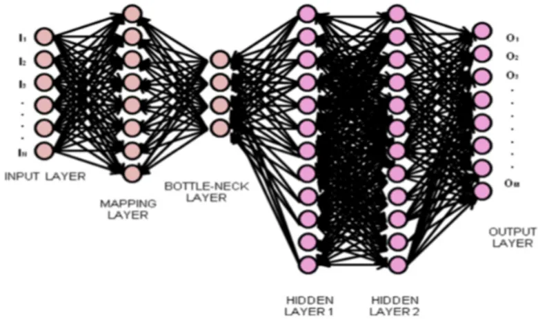
Figure 3.3: A three hidden layer autoassociative neural network

subspace would correspond exactly to linear PCA [80]. Also if the activa-tion funcactiva-tions in the bottleneck nodes were sigmoidal, the projecactiva-tion into the sub-space would still be severely constrained; only linear combinations of the inputs compressed by the sigmoid into the range [-1,1] could be rep-resented. Therefore the performance of an autoassociative neural network with only one internal layer of sigmoidal nodes is often no better than lin-ear PCA [81]. Starting from these premises, Kramer demonstrated that to perform an effective NLPCA, exactly one layer of sigmoidal nodes and two layers of weighted connections are required [75], as depicted in fig.3.3.

Such a network effectively performs a nonlinear principal component analysis, having the advantage of not being limited to linear transforma-tion, although it contains standard principal component analysis as a spe-cial case. Moreover, the dimensionality of the sub-space could be specified

(60)

Figure 3.4: The mapping and demapping layers of an autoassociative neural network

in advance of training the network. As the NLPCA method finds and elim-inates nonlinear correlations in the data, analogous to principal component analysis, this method can be used to reduce the dimensionality of a given data by removing its redundant information. Our intent is to apply this methodology to perform the dimensionality reduction of the large measure-ments vector typical of the hyper-spectral data. As illustrated in fig.3.4, the network can be viewed as two successive functional mapping networks. The first mapping network projects the original d dimensional data onto a lower dimensional sub-space defined by the activations of the units in the bottleneck layer. Because of the presence of nonlinear units, this mapping is essentially arbitrary, and in particular not restricted to being linear. Similarly the second demapping network defines an arbitrary mapping from

(61)

3.3 Nonlinear principal component analysis 55 the lower dimensional space back into the original d-dimensional space. Once the sum-of-squares error has reached its minimum, the projection in the low dimensional feature space was obtained from the outputs of the mapping layer. As the number of nodes in the input and output layers, as well as in the bottleneck layer, can be considered as a fixed parameter, the only varying value in the design of a autoassociative neural network are the number of nodes in the mapping layers. However, there is no definitive method for deciding a priori the dimensions of these layers. The number of mapping nodes is related to the complexity of the nonlinear functions that can be generated by the network. If too few mapping nodes are provided, accuracy might be low because the representational capacity of the network is limited. However, if there are too many mapping nodes, the network will be prone to “over-fitting”. In the following chapters, the use of the NLPCA, intended as a dimensionality reduction technique of very different types of hyper-spectral data, will be described for different cases.

(62)

(63)

Chapter 4

Land cover maps from AHS

dataset

4.1 Introduction

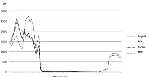
In this section we present the assessment of a methodology based on AANN with respect to more standard features extraction approaches such as Prin-cipal Component Analysis (PCA) and MNF (Minimum Noise Fraction). The study has been carried out for a set of hyper-spectral data collected by the Airborne Hyper-spectral line-Scanner radiometer (AHS) over a test site in Northeast Germany. This is a test area for which an extensive ground-truth was also available. The results have been quantitatively evaluated and critically analyzed either in terms of their capability of representing the hyper-spectral data with a reduced number of components or in terms of the accuracy obtained on the final derived product. This latter consists of a land cover classification map performed using another NN scheme, this time with the standard topology of a Multi-Layer Perceptron (MLP),

(64)

having as input the reduced vector provided by the AANN. It has to be observed that, dealing with a NN classification scheme, features extraction assumes an even more crucial role. Minimizing the number of inputs of a NN, avoiding significant loss of information, generally affects positively its mapping ability and computational efficiency. A network with fewer inputs has fewer adaptive parameters to be determined, which need a smaller train-ing set to be properly constrained. This leads to a network with improved generalization properties providing smoother mappings. In addition, a net-work with fewer weights may be faster to train. All these benefits make the reduction in the dimension of the input data a normal procedure when designing NN, even for a relatively low dimensional input space.

4.2 Data and methodology

The potential of AANN has been investigated for a set of data acquired by the INTA-AHS instrument, in the framework of the ESA AGRISAR measurement campaign [91]. The test site is the area of DEMMIN (Durable Environmental Multidisciplinary Monitoring Information Network). This is a consolidated test site located in Mecklenburg-Western Pomerania, in Northeast Germany, which is based on a group of farms within a farming association covering approximately 25,000 ha. The field sizes are very large in this area, in average 200-250 ha. The main crops grown are wheat, barley, rape, maize and sugar beet. The altitudinal range within the test site is around 50 m. The AHS has 80 spectral channels available in the visible, shortwave infrared and thermal infrared. The data processing level is the L1b (at-sensor radiance): the VIS/NIR/SWIR bands were converted to at

(65)

4.2 Data and methodology 59 sensor radiance applying the absolute calibration coefficients obtained in the laboratory. The MIR/TIR bands were converted to at-sensor radiance using the information from the onboard blackbodies and the spectral responsivity curves obtained by the AHS spectral calibration. The resulting files were converted to BSQ format + ENVI header and scaled to fit an unsigned integer data type. In this paper the acquisition taken on the 06/06/2006 has been considered. At that time 5 bands in the SWIR region became blind due to loose bonds in the detector array so they were not used in this study [82].

A double-stage processing has been applied to the data. In the first stage a features reduction has been performed by means of AANN, in the second stage the reduced measurement vector has been used as input to a new NN scheme for a pixel-based classification procedure. It has to be noted that the vector reduction should positively affects the training of the classification neural network algorithm under two points of view: it reduces both over-fitting and learning time. As far as the feature extraction is concerned, the comparison with PCA and MNF techniques has been carried out using processing libraries available within the ENVI package. Another important aspect regards the design of the network topologies, in particular how many units should be considered in the hidden layers. This is a crucial issue because using a too little number of units may weaken the capability of the network to perform the desired mapping. On the other hand, over-dimensioned hidden layers may lead to poor generalization properties. In this study, different strategies have been adopted. However, most of the efforts have been dedicated to the design of the AANN, being this aspect

(66)

the focus of the work. The number of neurons in the bottleneck layer was guided by the necessity of comparing the features extraction performance of different approaches. A preliminary analysis based on PCA was carried out to determine the number of PCA components containing most of the statistical information (more than 99%). For the sake of consistency, the same number was also considered for the NLPCA, hence for the units in the bottleneck layer, and for the MNF. The decision on the size of the intermediate hidden layers was based on a more extended analysis where the size was systematically varied and the corresponding autoassociative network mapping MSE error evaluated.

The size minimizing such an error was selected for determining the networks topology. Finally, for the network dedicated to the classification scheme, a more soft strategy among those already existent in literature has been chosen. In particular we considered the rule used by Palmason et al. [83] suggesting that the number of neurons in the hidden layer should be set as geometrical mean of the number of inputs and outputs, i.e., the square root of the product of the number of input features and the number of information classes.

4.3 Results

4.3.1 Feature extraction

According to Kramer [75], the AANN has been trained considering all pix-els in the image (2061000). After about 2000 epochs no significant decrease in the error could be noted so the training phase was stopped at that stage. From the PCA analysis it resulted that the first 5 PCA components

(67)

con-4.3 Results 61