Simulating highly non-linear dark matter dynamics beyond LCDM

ALMA MATER STUDIORUM

UNIVERSITÀ DEGLI STUDI DI BOLOGNA

_____________________________________________________

Dipartimento di Fisica e Astronomia

DOTTORATO DI RICERCA IN

ASTROFISICA

Ciclo XXXI

Tesi di Dottorato

SIMULATING HIGHLY NON-LINEAR

DARK MATTER DYNAMICS BEYOND ΛCDM

Presentata da: Matteo Nori

Coordinatore Dottorato:

Francesco Rosario Ferraro Supervisore: Marco Baldi

Esame finale anno 2019

Simulating highly non-linear

Dark Matter dynamics beyond

Λ

CDM

a dissertation presented by

Matteo Nori

The Department of Physics and Astronomy

Doctor of Philosophy in

Computational Cosmology

Alma Mater Studiorum - Bologna University Bologna, Italy

Thesis advisor: Dr. Marco Baldi Matteo Nori

Simulating highly non-linear

Dark Matter dynamics beyond

Λ

CDM

Abstract

Most of the presently available data regarding the structure and the properties of the Universe are well described within the standardΛCDM cosmological scenario. However, the underlying assumptions on which the standard framework is based on have been tested only over a restricted range of cosmic scales and cosmic epochs, and extremely severe fine-tuning problems still affect the rather peculiar choice of its parameters. Therefore, a wide range of extended cosmological models have been proposed in the literature to overcome these obstacles. Given the expected excellent high-precision data that will be available in the Precision Cosmology era, it will be possible to test such extensions of the standard cosmological model sys-tematically, to constrain them or rule them out. This will require the theoretical predictions of observable quantities to achieve the same outstanding quality for many competing non-standard cosmologies. In order to obtain such accuracy over a wide range of scales and epochs, the use of large and complex numerical simula-tions will represent an essential tool. In this thesis, we present the research activity carried out during three years of Ph.D., focused on the implementation and ap-plication of alternative cosmological models beyond-ΛCDM in the cosmological hydrodynamical code P-GADGET3. In particular, our work concerned the devel-opment of refined numerical routines to perform and improve simulations of two classes of strongly and non-linearly interacting dark matter scenarios: Fuzzy Dark Matter and Growing Neutrino Quintessence models.

Fuzzy Dark Matter (FDM) represents an alternative and intriguing description of the standard Cold Dark Matter (CDM) fluid, able to explain the lack of direct de-tection of dark matter particles in the GeV sector and to alleviate some of the small-scale tensions that still plagueΛCDM. In these models, the mass of the dark matter particle is so tiny that it exhibits quantum behaviour at cosmological scales. The typical decoherence and interference features, a peculiar characteristic of quantum systems, are encoded by an additional Quantum Potential (QP) in the dark matter dynamics. Given the strong non-linearity of the QP, full numerical simulations

Thesis advisor: Dr. Marco Baldi Matteo Nori of FDM models at high resolution have been limited so far to the investigation of individual objects with grid-based codes. Alternatively, when turning to cosmo-logically representative volumes, important approximations had to be introduced in N-body algorithms, due to the otherwise prohibitive computational cost of the simulations. In this thesis, we present the AX-GADGET module that we specif-ically developed for cosmological simulations of FDM, which is able to achieve high scalability and good performance by computing the QP-induced acceleration through refined Smoothed Particle Hydrodynamics (SPH) routines, with improved schemes to ensure precise and stable derivatives, thereby strongly alleviating the total computational load. Along with an overview of the algorithm, we show the comparison between theoretical predictions and numerical results, both for analyt-ical and cosmologanalyt-ical test cases, for whichAX-GADGETproves to be a reliable tool for numerical simulations of FDM systems. As an extension of theP-GADGET3 code,AX-GADGETinherits all the additional physics modules implemented up to date, opening a wide range of possibilities to constrain FDM models and to explore degeneracies with other physical phenomena. We then present the results of one major application of theAX-GADGET code, obtained from a simulation suite de-signed to constrain the FDM mass through Lyman-α forest observations and to characterise the statistical properties of collapsed objects. Both the Lyman-α con-straints and the characterisation of structure properties are obtained for the first time in the literature in an N-body set-up without approximating the FDM dynam-ics. Given the large halo sample available, we extract valuable information about how FDM affects the mass function, the shape and density distribution of dark matter haloes, showing for the first time that massive haloes become even more massive in FDM models by accreting matter at the expenses of smaller haloes.

Moving to the second class of models, we present a independent – and still ongo-ing – project involvongo-ing a generalised implementation of strongly coupled scenarios in theP-GADGET3 code. The approach of this new technique is very general and accounts for a wide range of models – like Coupled Dark Energy and Modified Gravity – that involve the solution of a non-linear Poisson equation. We extended to these models the implementation of the so-called Newton-Gauss-Seidel scheme, which is a tree-based iterative solver of differential equations, previously limited to the f (R) gravity case. We apply our generalised method to the case of Grow-ing Neutrino Quintessence (GNQ) models, where the neutrinos are coupled with a dark energy scalar field, that could not be successfully tested so far due to the numerical complexity of the problem. Our implementation improves numerical scalability and is flexible enough to accommodate custom specifications, covering a wide spectrum of models for future investigations.

Contents

I

Introduction

2

1 Modern Cosmology 3

1.1 The Homogeneous Universe . . . 4

1.2 The Inhomogeneous Universe: Linear growth of perturbations . . 15

1.3 The Inhomogeneous Universe: Non-linear growth of perturbations 26 2 The Simulated Universe 30 2.1 Computing the gravitational potential . . . 33

2.2 Evolving in time: Time-integration schemes . . . 36

2.3 From particle to fields: Smoothed Particle Hydrodynamics . . . 40

2.4 P-GADGET3 . . . 43

2.5 Beyond Cold Dark Matter . . . 47

II

Fuzzy Dark Matter

49

3.2 Simulation approach in the literature . . . 55

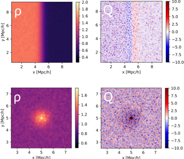
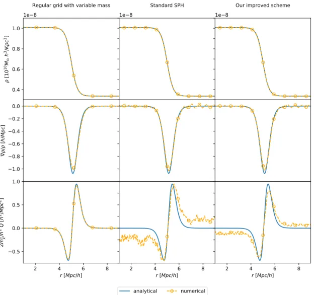
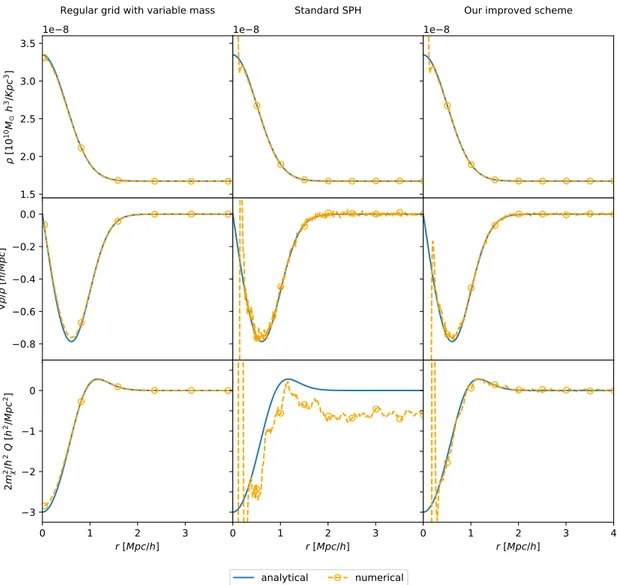
4 AX-Gadget 57 4.1 The algorithm . . . 58 4.2 Analytical tests . . . 65 4.2.1 1D Density Front . . . 66 4.2.2 3D Gaussian distribution . . . 71 4.2.3 Solitonic core . . . 72

4.3 Cosmological tests . . . 75

4.3.1 Quantum Potential effects on dynamics . . . 76

4.3.2 Quantum Potential and initial conditions . . . 81

4.3.3 Performance . . . 86

4.4 Summary of theAX-GADGETimplementation . . . 88

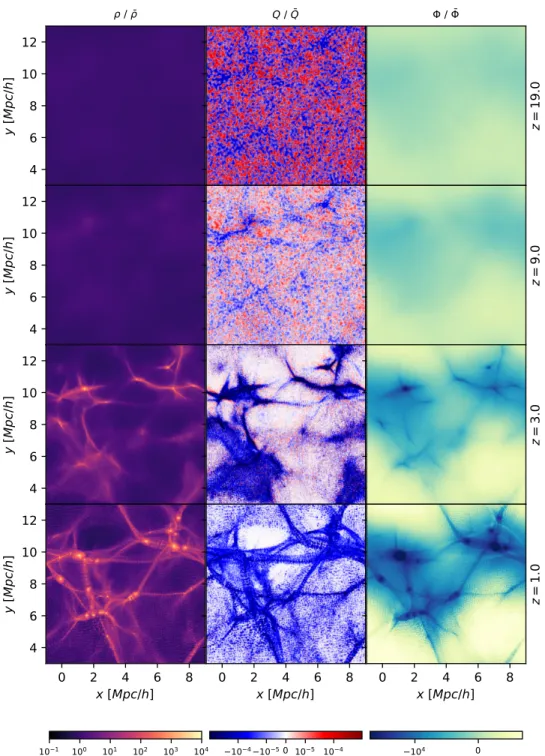
5 Lyman-α forest constraint and structure characterisation 91 5.1 Simulation suite . . . 92

5.1.1 Lyman-α forest simulations . . . 93

5.2 Matter and Lyman-α power spectrum . . . 96

5.2.1 Matter Power spectrum . . . 96

5.2.2 Lyman-α forest flux statistics . . . 99

5.3 Structure characterization . . . 103

5.3.1 Numerical Fragmentation . . . 103

5.3.2 Inter-simulations halo matching . . . 108

5.4 Summary on Lyman-α and structure characterisation . . . 117

III

Generalised Strongly Coupled models

120

6.2 f (R)-models and theMG-GADGETimplementation . . . 129

6.2.1 The multi-grid Newton–Gauss–Seidel solver . . . 131

6.3 Growing Neutrino Quintessence . . . 137

6.3.1 Our generalised implementation: the GNQ case . . . 139

IV

Conclusions

142

Part I

Scientific revolutions are inaugurated by a growing sense, [...] often restricted to a narrow subdivision of the scientific community, that an existing paradigm has ceased to func-tion adequately in the explorafunc-tion of an aspect of nature to which that paradigm itself had previously led the way.

Thomas Kuhn The Structure of Scientific Revolutions (1962)

1

Modern Cosmology

In the introduction of the controversial and irreverent essay Against Method ( Fey-erabend,1975), the Austrian philosopher Paul Feyerabend claims that “the history of science, after all, does not just consists of facts and conclusions drawn from facts. It also contains ideas, interpretations of facts, problems created by conflicting interpretations, mis-takes, and so on. On closer analysis, we even find that science knows no bare facts at all, but that the facts that enter our knowledge are already viewed in a certain way and are, therefore, essentially ideational”. Even if he criticized his contemporary fellow epis-temologist Thomas Kuhn for retreating from the more radical implications of his theory about the structure of scientific revolutions, they were both deeply inspired by the astonishing paradigm shift occurred in the first decades of the twentieth cen-tury, with the rise of the probabilistic quantum theories by Schrödinger and Planck in the micro-world and Einstein’s relativity theories of gravity in the macro-world.

Indeed, Einstein’s work completely re-framed the Newtonian notion of space and time, paving the way for the development of modern scientific cosmology. More than a hundred years later, our understanding of the origin, the evolution, and the eventual fate of the Universe has profoundly expanded. Nevertheless, the current cosmological paradigm has posed even more unanswered questions, em-phasizing the lack of a complete picture of the physical nature of the Universe.

In this chapter we will cover the main – in Feyerabend’s words – “facts” and “con-clusions drawn from facts”, as well as the “interpretations of facts”, that led to the devel-opment of the current standard cosmological model.

1.1

The Homogeneous Universe

In Einstein’s theory of gravity, space and time constitute two complementary as-pects of the same geometrical identity so that any event takes place on a four di-mensional space-time manifold. The distance between two events (t, x, y, z) and

(t + dt, x + dx, y + dy, z + dz) in Special Relativity (Einstein, 1905) is given by the line element

ds2=−c2dt2+ dx2+ dy2+ dz2 (1.1) and it is invariant under coordinate transformation. The properties of the flat space-time of Eq. 1.1 are then extended in General Relativity (Einstein,1916) to a more generic case, to account for curved geometries that incorporate the geo-metrical interpretation of the gravity sourced by a massive body

ds2= gi jdxidxj (1.2)

wheregi jis the metric of space-time anddx = (ct, x, y, z)is the position quadri-vector*.

The two Relativity theories are described through a complex but elegant tensor formalism and have interesting geometrical interpretations. In particular, General Relativity characterises how mass is able to curve space-time, influencing light and particle trajectories in its surroundings.

On curved manifolds, two vectors that are mutually parallel at a given point will not remain necessarily parallel when they are moved apart, in the same way in which the Eiffel Tower in Paris and its replica in Tokyo are nearly perpendicular to each other, despite both being safely perpendicular to the ground. The distortion of theλ coordinate of vectorA, that is parallel transported along theµcomponent of the basis, is quantified through the covariant derivative

∇µAλ =∂_µAλ+Γλ_µν Aν (1.3) where theΓλ_µν coefficients are defined as

Γλ_µν =1 2g

λσ(_∂

µg_σν+∂_νg_{σ µ}−∂_σg_µν) (1.4) and are called the Christoffel symbols.

Therefore, if the two parallel vectors are transported along closed circuits, they may point in different directions when they meet again at the origin. Imag-ine, for example, a closed circuit generated by two vectors X and Y with sides

[tX ,tY,−tX,−tY]regulated by a generic size parametert. In the limit oft→ 0, the transformationR(X ,Y )experienced by the vectorZtransported along such loop is described by the so-called Riemann curvature tensorRλ_µνσ

Rλ_µνσXµYνZσ = (R(X ,Y )Z)λ = (∇X∇YZ− ∇Y∇XZ− ∇XY−YXZ)λ (1.5)

that can be expressed as

Rλ_µνσ =∂_νΓλ_µσ−∂_σΓλ_µν+Γλ_νtΓt_µσ− Γλ_σtΓt_µν (1.6) in terms of the Christoffel symbols. The transformation generated by such geomet-rical effect is connected with the Ricci curvature tensor

R_µσ = Rν_µνσ (1.7)

In Einstein’s theory, the geometry of space-time is entirely described by the Ricci tensor and it is modified by the presence of energy and matter, as elegantly con-densed in the Einstein equation

R_µν−1

2gµνR = 8πG

c4 Tµν (1.8)

whereGis Newton’s constant and the mass and energy distribution sourcing the gravitational potential are enclosed in the stess-energy tensorT_µν.

Within a general space-time framework, the analytic solutions of Einstein equa-tion are extremely complex to be derived and, in the first attempts to describe the Universe, two assumptions were introduced. In particular, our role as Earth-based observers was assumed to be unprivileged with respect to other possible observers in the Universe, and combined with the isotropy hypothesis, considering the Uni-verse statistically similar in every direction. The union of the two constitutes the so-called Cosmological principle, which implies the homogeneity of the Universe at sufficiently large scales.

The translational and rotational symmetries implied by the Cosmological Prin-ciple can be used to rewrite the spatial part of the metricd⃗r = (dx, dy, dz)of Eq. 1.2 in spherical coordinates(dr, dθ, dϕ)as ds2=−c2dt2+ a2(t) [ dr2 1− Kr2+r 2(_dθ2_{+ sinθ}2_dϕ2)] _(1.9)

named Friedmann–Lemaître–Robertson–Walker (FLRW) metric. The curvature parameter K has units[L−2]and is related to the topological geometry of the space-time, that can be either flat (K = 0), closed (K > 0) or open (K < 0): in this three geometries, two rays of light that are locally parallel will remain parallel, converge or diverge, respectively. The dimensionless parametera(t) is the scale factor and accounts for the time-dependence of distances, allowing the fabric of space-time to contract or expand.

In fact, we can define the physical distance between two points as ⃗r = a(t) ˆr ∫ _dr √ 1− Kr2 = a(t) ˆr          arcsinhr forK < 0 r forK = 0 arcsinr forK > 0 (1.10)

and the comoving distance as

⃗x = a0

a(t)⃗r (1.11)

where the0subscript refers to the value at present time.

Depending on the specific case, physical processes are more elegantly described in the physical or the comoving frame: in order to recover one from the other it is useful to recall the definition of total derivative of a generic functionf with n

arguments{a1, a1, ...an} d dtf (a1, a1, ...an) = n

∑

where∂t is the partial derivative. Since total derivative is invariant under

coordi-nate transformation, we have that

     ∂tf (⃗r,t) =∂tf (a⃗x,t)− ˙ a a ( ⃗x·⃗∇x ) f (a⃗x,t) ⃗∇r= 1 a⃗∇x (1.13)

where we adopt the conventional dot operatora˙to represent the total time deriva-tive.

The velocities in comoving and physical coordinates are

⃗u = ˙⃗x (1.14)

respectively, where the factor

H(t)≡ a˙

a (1.16)

is the Hubble function, named after the American physicist Edwin Hubble, whose value at present time – the Hubble parameter H0 – is often conveniently reduced to

the dimensionless variableh = H0/(100 km/s/Mpc).

In 1929, Hubble was able to estimate the value of H0 using the observations

of several Cepheid variables collected together with Milton Humason, using the Hooker Telescope located at the Mount Wilson Observatory (Hubble,1929; Hub-ble and Humason,1931). Combining distance measures resulting from the intrin-sic Cepheid variability with the velocities, obtained from the Doppler redshift effect of their emission, he was able to prove not only that the objects observed belonged to extra-galactic systems – called nebulae at that time – but also that such systems were all moving away from Earth, with velocities proportional to their distance independently from their position in the sky.

The Doppler effect is the observed shift in the wavelengthλ of signals emitted by a moving source, that exhibit smaller (blueshift) or larger (redshift) wavelength with respect to the original one if the source is approaching or receding from the observer, respectively. In cosmology, the signals emitted by a source are redshifted by the expansion of space-time

z = dλ λ = dv v ≃ H dr v = Hdt = da a (1.17)

and this can be directly related to the scale factor

1 + z =a0

a (1.18)

as the redshift is de facto commonly used as a substitute for the scale factor itself. In Hubble’s work, the statistical estimate ofH0was derived from the liner

regres-sion between the physical velocity and the distance

exhibited by objects in nearby galaxies under the assumption of constantH(t) = H0.

This is considered the first observation of the expansion of the Universe: in fact, it is possible to describe the velocity of each object as

⃗v = H ⃗r + a ⃗u≃ H ⃗r (1.20)

where the contribution of the comoving velocity⃗uis considered to be negligible with respect to the cosmic drift and statistically irrelevant since it should be ran-domly distributed in the sample.

With the assumptions of the Cosmological Principle, the general metric of the space-time on the left-hand side of Einstein equation Eq. 1.8 can be reduced to a more symmetric and simple form that involves two main components: a curva-tureK and a scale factora(t)describing the geometry of the space and its intrinsic expansion rate, respectively.

In order to have a complete picture of evolution of the Universe, let us now turn to the right-hand side of Einstein equation: the stress-energy tensorT_µν. It is useful to describe – at first – the energy and matter content of the Universe as a single and perfect fluid, which does not experience conduction (T0,ν = Tµ,0= 0)

nor shear stresses (T_µν= 0 :µ̸=ν), such that the stress-energy tensor reads

T_µν = diag(ρc2, P, P, P) (1.21)

whereρ andPare the density and pressure of the fluid, respectively.

Solving Eq. 1.8 for the T00 component ant for its trace trT, we obtain the two

Friedmann Equations (Friedmann,1924)

H2= 8πG 3 ρ− Kc2 a2 (1.22) ˙ H =−4πG ( ρ+ P c2 ) +Kc 2 a2 (1.23)

from which we can derive ¨ a a =− 4π 3 G ( ρ+ 3P c2 ) (1.24) to explicit the second derivative of the scalar factor.

Taking the derivative of Eq. 1.22 and substituting it in Eq. 1.23 we find

∂tρ+ 3H ( ρ+ P c2 ) = 0 (1.25)

which exemplifies an interesting property of the Universe under study. In fact, the previous equation can be rewritten as the definition of adiabatic expansion

dU + PdV = 0 (1.26)

where we recognize the internal energyU =ρc2a3and the volumeV = a3, mean-ing that – in this framework – the Universe is a closed system: matter and energy cannot be lost to or gained from an external source.

Let us note from Eq. 1.23 that a static solution of the two Friedmann equations exists, but it requires

H = 0⇔ P = −ρc2 (1.27)

˙

H = 0⇔ρ = 3Kc

2

8πGa2 (1.28)

meaning that the densityρ or the pressurePshould be negative, even if both are expected to be positive for a standard fluid. This was one of the reasons – among others – that led Einstein to introduce a cosmological constant Λ and the relative density componentρΛ =Λc2/8πGthrough the invariant transformation of

coor-dinates (Einstein,1917)

P→ ˜P + P_Λ (1.29)

that would effectively resemble a fluid with negative pressureP_Λ=−ρ_Λc2.

In order to divide the single fluid in several fluid speciesi, we define each equa-tion of statePi= Pi(ρi)in the form of

Pi= wiρic2 (1.31)

wherewiis a parameter describing the nature of the fluid component that can be

related to the sound velocitycs,i wi=

c2_s,i c2 =

∂ρiPi

c2 (1.32)

and to the time evolution of each species density

ρi=ρi,0a−3(1+wi) (1.33)

as obtained from Eq. 1.25. Rearranging Eq. 1.26, it is also possible to see that the parameterwidetermines how the internal energy changes with respect to a volume

variation

dUi

dV =−Pi=−wiρic

2 _(1.34)

in the case of adiabatic expansion. Therefore, it is possible to identify three main different behaviours:

• Non-relativistic matter wmat = 0⇒ρmat ∝ a−3:

the internal energy is dominated by mass contributionUi≃ mic2, which is

constant in time, implying that the fluid is pressure-less and its density scales as the inverse of the volume;

• Relativistic matter and radiation wrad= 1/3⇒ρrad∝ a−4:

the redshift effect contributes with an additionala−1factor to the volume scal-ing, identifying this case as radiation and ultra-relativistic particles in thermal equilibrium;

• Cosmological constant w_Λ=−1 ⇒ρ_Λ∝ 1:

this behaviour is consistent with the properties of the cosmological constant of negative pressure and of constant density as previously described.

Since matter, radiation and the cosmological constant density evolutions scale differently with respect to the cosmic expansion, the Universe lifetime can be di-vided into three eras with respect to the dominant component at each time. Given a non-zero value forρmat,0,ρrad,0andρΛ,0, there exist three crossover moments in

which the densities of a pair of the species equate. These are identified with the three equality redshifts

• Matter–Radiation equality 1 + zeq=ρmat,0/ρrad,0

• Radiation–Λequality 1 + zrad,Λ= (

ρΛ,0/ρrad,0 )1/4

• Matter–Λequality 1 + zmat,Λ= (

ρΛ,0/ρmat,0 )1/3

where matter–radiation equality is referred as equality conventionally when not specified otherwise. In the degenerate case for which the three redshifts are equal – i.e. zeq= zrad,Λ= zmat,Λ⇒ρmat,04 =ρrad,03 ρΛ,0 –, there is a transition from

radia-tion to cosmological constant dominated era. A matter dominated era can break through between the two ifρ4

mat,0≥ρrad,03 ρΛ,0, so that the first era during cosmic

evolution is characterised by radiation, followed by matter and later on by the cos-mological constant.

To better analyse the relative contribution of the different species to the cosmic evolution let us switch to dimensionless coordinates, in particular defining the use-ful dimensionless density parameters Ωmat,ΩradandΩΛ as

Ωi= ρi ρc

(1.35) and total density parameter as

Ωtot= 1 ρc

∑

∑

where we defined also

ρc= 3H2

8πG (1.37)

as the critical density.

The Friedmann equations can be rewritten as

1 + Kc 2 a2_H2 =

∑

∑

where is underlined the dependence of the curvatureK and the scale factor accel-erationa¨on the content of the Universe.

It appears clearly from the previous equations that, in a Universe with only mat-ter and radiation – treated as perfect fluids –, the acceleration of the scale factor is always negative. In fact, three scenarios can be outlined for the expansion dynam-ics – keeping in mind that Hubble’s result confirmed the cosmic expansionH0> 0–,

in particular studying how the cosmic acceleration a¨ changes with respect to the relative weight of the cosmological constant in the total energy-matter content of the Universe:

• a < 0¨ forΩΛ < 1₂Ωmat+Ωrad: for all the cosmic eras when the cosmological constant is (still) irrelevant, matter and radiation decelerate cosmic expan-sion.

• a = 0¨ forΩΛ=1₂Ωmat+Ωrad: this case represents the flex point of the acceler-ated expansion onset and it is eventually reached if a non-zero cosmological constant component exists.

• a > 0¨ forΩΛ> 1₂Ωmat+Ωrad: when the cosmological constant becomes the dominant component in the Universe, the Universe expands at an exponen-tially accelerated pace without end.

It is also possible to link the three different values for the curvature K at each time to the total density parameterΩtot:

• Ωtot< 1⇒ K < 0:

the curvature of space-time geometry induced by the content of the Universe is not enough to compensate the one deriving from cosmic expansion, and it results in an open geometry and ever-expanding Universe.

• Ωtot= 1⇒ K = 0:

in this case, all species contributions sum up to the critical density, exactly balancing the expansion and recovering a flat Euclidean geometry.

• Ωtot> 1⇒ K > 0:

if the critical density is surpassed, the curvature induced on the space-time overtake the expansion of the Universe and the geometry is closed. A turning point is eventually reached in the case of null cosmological constantΩΛ= 0

and the Universe starts to shrink towards a singularity – often referred to as Big Crunch –.

To summarize, the symmetries assumed for the metric of the space-time of Gen-eral Relativity are combined with the perfect fluid description of the energy-matter content of the Universe into the Friedmann equations, that represent the master equations for the dynamics of an expanding Universe and provide several predic-tions for the past, present and future evolution of the Universe as well as its in-trinsic geometrical properties. The description of the Universe is crucially related to the present value of the Hubble parameterH0and the three density parameters

Ωi,0, in order to solve

( H H0 )2 =Ωrad,0(1 + z)4+Ωmat,0(1 + z)3+ ( 1−

∑

1.2

The Inhomogeneous Universe:

Linear growth of perturbations

As detailed in the previous Section, the results obtained through the Friedmann equations are valid as long as the Cosmic principle holds – i.e. if the homogeneous assumption is legitimate – so that the evolution of matter and energy densities can be described through their mean value.

In 1964, Arno Penzias and Robert Wilson, with the Holmdel horn antenna at the Bell Labs in Holmdel Township, serendipitously discovered an electromag-netic emission in the microwave band, isotropically distributed as a micro-wave background (Penzias and Wilson,1965): it was the first observation of the Cosmic Microwave Background (CMB) already hypothesized byAlpher et al.(1948);Alpher and Herman(1948).

After the discovery of the expansion of the Universe by Hubble, it was still de-bated whether this result suggested that the Universe was smaller in earlier times, thus implying a singularity fora→ 0– i.e. the Big Bang or, in Lemaître’s words, the Cosmic Egg (Lemaître,1933) –, or that the expansion was not an adiabatic process as stated by Eq. 1.26 and matter and energy were constantly input to reach a Steady State (Bondi and Gold,1948).

It was already evident at the time that, if the Universe was smaller throughout its history, it should also be hotter and denser. Therefore, it exists a moment in the past when the protons and electrons were so energetic to be unable to bound and form atoms, continuously scattering with photons in a hot state called plasma, thus effectively impeding light transmission and making the Universe an opaque medium. When the temperature and the density of the plasma lowered enough due to the cosmic expansion, electrons and protons combined into atoms in a process identified as recombination, suddenly clearing the path to the photons that eventu-ally were detected by Penzias and Wilson billions of years later and still permeate the Universe.

The observed emission had the characteristic Planckian shape of a perfect black body thermal emission with a peak temperature of2.7K, as measured by the NASA COBE experiment in 1992 (Smoot et al.,1992). Knowing the temperature required

for the recombination process (T ∼ 3000 K) and the evolution of radiation tem-perature during cosmic expansion (T = T0(1 + z)), the CMB was identified as the

relic radiation emitted during the recombination era when the Universe was ap-proximately379, 000years old, at redshiftz∼ 1100, that contributes today to the total energy-matter content withΩrad,0= 9.2× 10−5. Therefore, the discovery of the CMB confirmed that the homogeneity approximation was correct and that the Universe has expanded from a Hot Big Bang state, contradicting the Steady State hypothesis.

The homogeneity of the CMB, however, was expected to break down by tiny fluctuations derived from the dynamical equilibrium of the plasma, since a per-fectly homogeneous Universe would not feature the inhomogeneities that eventu-ally turn into planets, galaxies and the structures surrounded by empty space we see today. The presence of acoustic oscillations was predicted as a possible effect in the CMB in the late 1960s (Sakharov,1966) and further studies (Bond and Efstathiou,

1984;Efstathiou and Bond,1986;Hu and White,1996) investigated possible meth-ods to use the scale of inhomogeneities as a standard ruler as we will describe be-low(Kamionkowski et al.,1994;Jungman et al.,1996).

Since it is possible to relate the temperature fluctuations with the density ones, in order to study the deviations of T andρ from the homogeneous background solutionsTbandρb(a) =ρb,0a−3, we define the temperature contrast

∆(⃗x) = T (⃗x)− Tb

T_b (1.41)

and the density contrast

δ(⃗x, a) =ρ(⃗x, a)−ρb(a) ρb(a)

(1.42) in each point⃗xof the space. Moreover, since fluctuations of the early Universe dis-tribution are nearly acoustic, it is more convenient to perform perturbation analy-sis in Fourier space, where the density contrast reads

δk= 1 (2π)3

∫

and its2-point correlation function is

P(k)≡ ⟨δ_k2⟩ = ⟨ ∫

d(⃗x−⃗x′) δ(⃗x)δ(⃗x′) ei⃗k·(⃗x−⃗x′)⟩ (1.44) often referred as Power Spectrum (PS)†, where the angle brackets<>indicate ensem-ble average over smaller patches of the Universe volume. The2-point correlation function related to temperature perturbations is more conveniently represented in spherical coordinates, thus called Angular Power Spectrum, where the polar and az-imuthal angles(θ,ϕ)are expressed through the multiple moment and order(l, m)

of the spherical harmonic

C_l=⟨ 1 2l + 1 l

∑

and the angular scale can be derived through180◦/l.

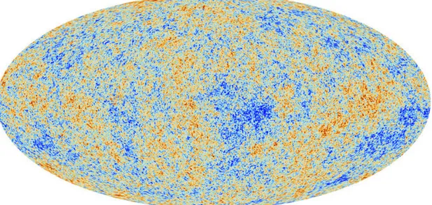
In Fig. 1.1 the projected sky map of the δT _{fluctuations as seen by the Planck}

experiment – upper panel, red and blue for positive and negative values, respec-tively – and the relative Angular PS are represented, the latter plotted in terms of T₀2 l(l + 1) Cl as function of both l and the angular scale of separation – bottom

panel –.

The Angular PS has very distinctive features, mainly represented by an initial slope, several peaks of different heights and a damping tail. These features, called Barionic Acoustic Oscillations (BAO), can be described within a single theoretical pic-ture in which baryonic matter and radiation acoustically oscillate in the primordial plasma, driven by the opposite influence of gravity and radiation pressure. Odd and even peaks represent the maximal compression and rarefaction states due to gravi-tational attraction and pressure repulsion, respectively‡. The CMB photons, once recombination occurs, freely stream through the Universe retaining information on this oscillatory pattern.

The correlation between two points of the CMB map is a function of their

angu-†_{Note thatP(k) = P(|⃗k|)because of isotropy.}

‡_{Compression and rarefaction states have positive and negative temperature fluctuations, but}

Figure 1.1: The Cosmic Microwave Baground: a map of the temperature deviations from the mean

value (top panel) and the Angular Power Spectrum of such fluctuations (bottom panel). Credit: ESA and PLANCK Collaboration (Planck Collaboration,2018)

lar separation compared to the size of the Universe at the time of recombination, approximately corresponding tol∼ 50atz∼ 1100: for example, points with small angular separation –l≫ 50– experienced several oscillation cycles while very dis-tant points –l≪ 50– did not even start to oscillate.

In this sense, the shape at low multipoles still holds information of the primordial spectrum of the early Universe, which is well described by a (nearly) scale invariant relation

Cl = Al(l/l0)ns−1 (1.46)

that translates into a primordial matter PS

P(k) = As(k/k0)ns (1.47)

where the parametersAs (Al) andnsrepresenting the scalar (angular) amplitude and

the scalar spectral index, respectively, can be fitted to the data.

The first peak represents the leading compressed state given by matter gravita-tional in-fall and was observed for the first time by the high-altitude balloon experi-ment BOOMERanG flying around the Antarctic South Pole in the years 1998-2003 (de Bernardis et al.,2000;Masi et al.,2002). Given the size of the Universe, its age, matter and radiation content, it is possible to calculate the expected momentl_firstexp

of this first peak at recombination and use it as a standard ruler. Therefore, any dis-crepancy between the observed value l_firstobs and the theoretical one would indicate a curvature of the space-time K that modified the path of CMB photons, either shrinking –l_firstobs < l_firstexp – or expanding –lobs_first> l_firstexp – the projected size of such sig-nal. Hence, with the use of the first peak only it was possible to fix the curvatureK

to good precision; however, it was impossible to break down the contribution of each species represented by the density parametersΩi, for which exploiting higher order peaks is required.

The second peak denotes the first bounce induced by radiative pressure and was captured by the WMAP satellite in 2001 (Bennett et al.,2013). In a plasma where the electrons and protons contribution is negligible with respect to radiation, the first and the second peak would have the same height in an almost symmetric state,

but this is not the case: the symmetry, in fact, is broken by gravity, that enhances the collapse (first peak) with respect to the rarefaction (second peak). Therefore, the ratio between the first two peaks is sensitive to the relative abundance of the species belonging to the plasma.

If the Universe at recombination consisted only in plasma, the other acoustic peaks would be a sequence of exponentially decaying higher order harmonics of the first and the second peak, where the damping originates from the photon random-walk diffusion in the recombination process that effectively suppresses tempera-ture correlation abovelS≳ 800– called Silk damping, after the British astrophysicist

Joseph Silk (Silk,1968) –.

The measurement of higher order peaks, performed by the Planck satellite from 2009 to 2018, highlighted an excess power in the third peak and a lack of power in the tail with respect to the primary and secondary peaks. Since the third peak is related to the matter re-collapse after the first acoustic oscillation, a higher power in this peak suggests that the gravitational well originated with the first collapse was not entirely restored by radiation pressure bounce. Such asymmetry can be explained with the addition of another fluid that is coupled gravitationally with the plasma but does not experience radiative pressure, enhancing consecutive matter in-falls, which can be associated with a form of dark matter.

While – at the turn of the third millennium – the CMB was providing an im-pressive amount of crucial information about the early and present Universe, two independent projects were able to prove that the rate of expansion of the Universe is not constant and is indeed accelerated. In 1998 the Supernova Cosmology Project (Perlmutter et al.,1999;Schmidt et al.,1998) at Lawrence Berkeley National Labo-ratory and the High-Z Supernova Search Team (Riess et al.,1998) at the Australian National University both used Supernovae of type Ia to extend Hubble’s diagram to more considerable distances, observing a deviation at high redshifts from the linear law that implied a variation of the rate of expansion. Supernovae Ia, as the Cepheid variables, are considered standard candles as their distance can be inferred through their luminosity properties and the hydrogen and silicon lines of the emit-ted spectrum can be used to determine their redshift. The distance-redshift relation

obtained by the high-z Supernovae was consistent with an accelerating expansion and was best fitted by the combination of the density parametersΩmat ∼ 0.3and

ΩΛ∼ 0.7when combined with CMB results.

By the time of this measurement, other observations spanning through many orders of magnitude in scale were compatible with the presence of a cold and dark form of matter (CDM) – a not-strongly electromagnetically interacting particle or a gravitational quid that mirrors the effect of such fluid –. These are related to dy-namical properties of systems, as e.g. the inner dynamics of galaxy clusters (Zwicky,

1937;Clowe et al.,2006) and the rotation curves of spiral galaxies (Rubin et al.,1980;

Bosma,1981;Persic et al.,1996), to the gravitational impact on the underlying ge-ometry of space-time, as strong gravitational lensing of individual massive objects (Koopmans and Treu,2003) and the weak gravitational lensing arising from the large-scale matter distribution (Mateo,1998;Heymans et al.,2013;Planck Collabo-ration et al.,2015;Hildebrandt et al.,2017), as well as on the clustering of luminous galaxies (see e.g.Bel et al.,2014;Alam et al.,2017), on the abundance of massive clus-ters (Kashlinsky,1998) and their large-scale velocity field (Bahcall and Fan,1998). To summarise, the CMB Angular PS and the Supernovae Ia projects provided an incredible source of information regarding the past and present Universe. It allowed to estimate the density parameters Ωrad, Ωmat – in its components Ωbar andΩcdm –, the curvature K, the cosmological constant density contributionΩΛ

and equation of state w_Λ, as well as the present value of the Hubble parameterH0,

the age of the universe and the primordial PS scalar parametersAs and ns. The

parameters mentioned above are reported in Tab. 1.1 as measured by the 2018 release of the Planck collaboration results.

The theoretical cosmological framework originated by these results is called Λ -CDM, and describe the Universe as composed of radiation and standard baryonic matter, together with cold and dark matter – that enhances the gravitational col-lapse and drives structure formation – and a non-zero cosmological constant Λ with equation of statew_Λ =−1, generally called dark energy, prompting the late-time cosmic expansion acceleration.

As seen in the previous paragraphs, the CMB Angular PS is consistent with a primordial density PS in the form of

P(k) = Askns (1.48)

where the exponentns estimated by Planck (Planck Collaboration,2018) is very

close, even if not equal, to unity. A value ofns= 1is characteristic of a perfect

scale-invariant system, where the perturbations are equally likely to arise irrespectively of the scale considered. The scale-invariance of the primordial PS and the possible deviations from it are intimately connected with the properties of the Universe at early times.

The flatness of the space-time, the overall temperature homogeneity of the CMB and the near scale invariance of its perturbations could all be considered curious and peculiar properties from an a priori point of view. Since they require a particular set of cosmological parameters that in principle could have any value, such coinci-dence poses a fine-tuning problem to the standard cosmological model. Due to the cosmic expansion, progressively more and more regions of the Universe are casu-ally connected: it is natural to wonder how previously separated regions shared the same temperature and were characterised by energy-matter content that adds up exactly to the critical density preserving the Universe flatness.

It is now commonly accepted that approximately between10−36 and10−32 sec-onds after the Big Bang the Universe experienced a remarkably rapid exponential expansion by a factor∼ 1026_{. A similar mechanism would have put in causal contact}

– thus in thermal equilibrium, given enough time – very distant regions in the Uni-verse and would have also stretched any given initial curvature to an almost flat

ge-Table 1.1: Cosmological parameters as measured (or derived) by the Planck Collaboration in

com-bination with BAO and Supernovae Ia measurements (seePlanck Collaboration,2018, for detail).

Ωrad,0 Ωbar,0 Ωcdm,0 ΩΛ,0 wΛ

(9.2± 0.2) × 10−5 0.0490± 0.0007 0.261 ± 0.004 0.689 ± 0.006 −1.03 ± 0.03

Kc2/ ˙a2₀ h Age[Gyr] As× 109 ns

ometry. The idea of such cosmic inflation was proposed by Alan Guth (Guth,1981), Andrei Linde (Linde,1982) and Alexei Starobinsky (Starobinsky,1982) among oth-ers. In these models, the Universe faced a phase transition, described by the dynam-ical evolution of a scalar field – called inflaton – under the influence of a potential with multiple minima. In this picture, inflation is the exponential expansion of the Universe induced by the shift of the field from a local minimum of the potential to another one. However, despite being commonly accepted and consistent with data, experimental confirmation of the particular physical mechanism have yet to be found, and many inflationary models are still competing.

The set of equations that defines the density and velocity evolution in comoving coordinates of the matter fluid after recombination is

                 ˙

ρ+ 3Hρ+⃗∇ · (ρ⃗u) = 0 Continuity Equation

˙ ⃗u + 2H⃗u + ( ⃗u·⃗∇ ) ⃗u =−⃗∇P a2ρ− ⃗∇Φ a2 Euler Equation P = P (ρ) Equation of state ∇2_{Φ = 4πGa}2_(ρ−ρ b) Poisson Equation (1.49)

which is closed by the background evolution of the Hubble function of Eq. 1.40; the variableΦrepresents the gravitational potential that satisfies the usual Poisson equation (Peebles,1980).

The stationary – but unstable – solution of this system is a perfectly homoge-neous density distribution

             ρ(⃗x) =ρb=ρb,0a−3 u(⃗x) = 0 P = const Φ = 0 (1.50)

We are interested now in perturbing such background solution, in order to study the linearised evolution of the density contrastδ(a)defined in Eq. 1.42, which will be valid only in the regime of small perturbations|δ| << 1(for a complete review on the growth of linear density perturbation see e.g.Peebles,1993;Peacock,1999, to which we refer for details). If we take the time derivative of the Continuity Equa-tion, apply the divergence of the Euler Equation and combine the two, substituting the pressure and gravitational potential, we obtain

¨ δ+ 2H ˙δ+c 2 s a2∇ 2_{δ− 4π} Gρbδ = 0 (1.51)

that, expressed in Fourier space using the definition in Eq. 1.43, reads

¨ δk+ 2H ˙δk+δk ( k2c2_s a2 − 4πGρb ) = 0 (1.52)

that describes the linear evolution of density perturbation.

This equation features a stationary solution, identified by a periodic density per-turbation characterized by 2π kJ =λJ = cs a √ π Gρb = 2πcs aH √ 2 3Ωm (1.53)

called Jeans length, that represents the scale at which the collapse induced by gravity is balanced by the fluid pressure.

As a reference, let us focus on the case of a pressure-less matter fluid, for which

c2_s,mat = c2wmat = 0. It is interesting to notice that for a static Universe – i.e.H = 0–,

Eq. 1.52 reduces to

¨

δk= 4πGρb,0 δk (1.54)

whose solution is given by the linear combination of

D+(k,t) =δk,0e+ t √ 4πGρb,0 _(1.55) D₋(k,t) =δ_k,0e− t √ 4πGρb,0 _(1.56)

where D+(k, a) and D−(k, a) are the density perturbation growing and decaying

mode, respectively. In this case, the growth of perturbation is exponential in time. Instead, in the case of an expanding Universe and – in particular – in the matter dominated eraΩmat ≃ 1, we have that the Hubble function obtained from Eq. 1.40 satisfies

H = H0(a/a0)−3/2⇒ a = a0(t/t0)2/3 (1.57)

and the solution of Eq. 1.52 is a linear combination of

D+(k, a) =δk,0a (t) (1.58)

D₋(k, a) =δk,0a (t)−3/2 (1.59)

where the growth of perturbation is now proportional to the scale factora. The growth is slower with respect to the exponential one of the static Universe, since the gravitational collapse of structures has to overcome the expansion of space-time and the two mechanisms have opposite effect on structure formation§.

It is useful to recall that the CMB temperature fluctuations are of the order10−5

and can be mapped into baryonic density fluctuations of comparable intensity. If the total matter content of the Universe consisted in baryons exclusively, the den-sity perturbation would have grown fromδ ∼ 10−5 at recombination – happened at z∼ 1100 – to δ ∼ 10−2 at the present day, thus implying the complete linear evolution of perturbations and the absence of non-linear structures in the present Universe.

Such estimation is quite heuristic, but it well illustrates the need of a gravitational mechanism that is able to accelerate baryonic matter collapse into the complex struc-tures that we observe and are part of today: this is one of the primary motivation supporting the existence of non-baryonic dark matter.

§_{For this reason, the friction term2Hδ}

1.3

The Inhomogeneous Universe:

Non-linear growth of perturbations

On an analytical level, it is quite difficult to venture beyond the linear approxima-tion and solve exactly the evoluapproxima-tion of density perturbaapproxima-tions when these become comparable, or exceed, the background density value. Nevertheless, it exists a sim-ple and integrable model that describes the formation of bounded gravitational structures, called Spherical collapse model (Gunn and Gott,1972). For a detailed description of the model we are here going to review see e.g. Peebles(1993);Coles and Lucchin(2002).

Imagine to carve an over-dense spherical region in a spatially flat and matter-dominated universe – i.e. Ωmat,0 ≃ 1–: the growth of the spherical density is in-dependent from the background solution and effectively evolves as if it was a sub-Universe with its own density parameter Ωmat,0˜ > 1 and, consequently, positive curvature. In this framework, the background evolution of such sub-Universe is described by Eq. 1.40 and it reads

H = H0 [ ˜ Ωmat,0R−3+(1− ˜Ωmat,0 ) R−2]1/2 (1.60) whereRis the analogue of the scale factorafor the sub-Universe andtis character-istic time of the collapse. It is possible to express Eq. 1.60 in the parametric form

  

R (θ) = A (1− cosθ)

t (θ) = B (θ− sinθ) (1.61)

through the dimensionless development angle parameterθ ∈ [0,2π]and two factors

               A = R0 ˜ Ωmat,0 2(Ωmat,0˜ − 1) B = Ωmat,0˜ 2H0 (_˜ Ωmat,0− 1)3/2 (1.62)

that are defined by the boundary condition atR = R0andH = H0.

It is clear from Eq. 1.61 that the over-density expands until it reaches a turn-around point, defined by

Rmax= 2 A (1.63)

tmax =πB (1.64)

corresponding to the scale factor

Rmax = ( 3 2H0tmax )2/3 = ( 3π 4 ˜ Ωmat,0 )2/3 ₍ ˜ Ωmat,0− 1)−1 (1.65)

Aftertmax, it starts to fold back and eventually ends at the final collapsed

Rcol = 0 (1.66)

tcol= 2π B (1.67)

singularity state.

The density ratio between the collapsing object and the background evolves as

ρ ρb = Ωmat,0˜ ρc/R −3 ρc/a−3 = ˜Ωmat,0 (_a R )3 (1.68) that for the turn-around point is

ρmax ρb

= 9π

2

16 ≃ 5.55 (1.69)

meaning that a spherical perturbation is 555% more dense than the background when it enters the collapsing phase.

In this simple model there is no pressure to prevent the final singularity state. However, the singular state is not physically reached and the collapse stops once the virial condition

is satisfied, whereK andU are the kinetic and potential energy of the system, re-spectively. Therefore, after virialization,R (t > tvir)simply saturates to the constant valueRvir. For a spherical configuration, the potential energy is

U (R) =−3GM

2

5R2 (1.71)

that accounts for the total energyE = U + K att = tmax, since at the turn-around

point the sphere stands still – i.e. _R˙_{max = 0 ⇒ K (Rmax) = 0 –. In this process}

the total energy is conserved, thus we can easily retrieve the kinetic energy of the virialized state to obtain the scale relation

Rvir: 2K (Rvir) = 2 [U (Rmax)− U (Rvir)]

!

=−U (Rvir) ⇒ Rvir= Rmax

2 (1.72)

that characterizes such state.

Using the definition of Eq. 1.61, virialization happens at

θvir: A (1− cosθvir) = A ∧ (θvir>π) ⇒ θvir= 3π

2 (1.73)

that correspond to a time interval of

tvir tmax = ( avir amax )3/2 = ( 3 2+ 1 π ) ≃ 1.81 (1.74)

The density contrast with the background is

ρ(t = tvir) ρb = ρvir ρb =ρmax ρb ( Rvir Rmax )3( avir amax )3 = 9π 4 (3π+ 2)≃ 145 (1.75)

in the virialized state and

ρ(t = tcol) ρb = ρcol ρb = ρmax ρb ( Rvir Rmax )3( acol amax )3 = 18π2≃ 178 (1.76)

at the collapse time.

that perturbations can be considered gravitationally bound in non-linear structures when they become150− 180times denser with respect to the background density.

The extent of the failure of linear extrapolation can be appreciated if we contrast the exact non-linear density ratio with the one obtained by linearisation

ρ ρb   lin = 1 + 3 20 ( 6π t tmax )2/3 (1.77) that for the turn-around and final times are

ρmax ρb   lin = 1 + 3 20(6π) 2/3_{≃ 2.06} (1.78) ρcol ρb   lin = 1 + 3 20(12π) 2/3_{≃ 2.686} (1.79) meaning that the linear break down is already significant at the time of turn-around.

To summarise, the spherical collapse represents a valuable analytical result that describes how collapsed systems form in an expanding Universe. Even if the scal-ing relations obtained as well as the timscal-ings and the order of magnitude of density and size as compared to the background can be used in observable estimations, this solution refers to a highly idealised set-up. A physical cosmological system features multiple perturbations at various scales with no particular symmetry, thus hinder-ing the possibility to solve the density evolution analytically. Moreover, we showed that the linear approximation might deviate seriously from the exact non-linear so-lution, hence representing a valid alternative only at early times and on large scales. For this reasons, starting from the ‘60s, the exploration of the non-linear regime relied more and more on a different tool that has proven to be essential in the in-vestigation of the Universe evolution: numerical simulations.

2

The Simulated Universe

The dramatic improvements of our understanding of the Cosmos have prompted by the comparison between ground-breaking observational data – e.g. the Hubble Cepheids observation, the CMB and the results of the Supernovae Ia projects – with the forecast of the theoretical models of the Universe. However, in order to fully exploit the tremendous increment of the quantity and quality of observational data that new technologies allow for, it is required to have equally reliable and precise theoretical predictions of the key observables of interest.

The impossibility to rely on robust and general analytical results in the non-linear regime led to the implementation of numerical simulations that, with the thriving of computational power, now play a crucial role in the estimation of cos-mological observables regarding the formation and evolution of collapsed systems and the expected forecast related to future experiments design.

establish-Figure 2.1: The most important cosmological simulations from 1970 to 2010 are plotted year-wise

against their particle number. The numerical strategies related to the gravitational potential evalu-ation are represented by the different marker as described in the legend. Credit: Debora Sijacki

ment ofΛCDM as the standard cosmological scenario, providing decisive predic-tions on the non-linear structure formation driven by the presence of CDM and on the role of dark energy in the late-time accelerated expansion of the Universe.

The combined effects of the development of advanced numerical methods and the availability of increasing technological resources have induced the exponential evolution of simulation complexity and predictive power. The accuracy of numer-ical simulations of collapsed objects dynamics and large-scale structures formation has experienced a striking improvement during the years, as schematically por-trayed in Fig. 2.1, where the most important simulations milestones in a 40-year lapse of time are plotted against their number of particles – i.e. the smallest singu-lar components resolved in the system –.

Consistently with the resolution obtainable at the time, several systems have been the target of N-body simulations in the literature. First were investigated the formation and the dynamics of galaxy clusters (see e.g.Aarseth,1963;Peebles,

1970;White,1976;Aarseth et al.,1979;Frenk et al.,1983;Davis et al.,1985;White

et al.,1987) as well as their density and velocity statistical analysis (see e.g.Miyoshi

and Kihara,1975;Efstathiou and Eastwood,1981;Davis et al.,1985;Carlberg and Couchman,1989;Zurek et al.,1994). In the early ‘90s, the comparison between the large-scale correlation of galaxies simulated with the observations available already suggested a tension if no cosmological constant was taken into account (Maddox

et al.,1990;Efstathiou et al.,1990;Suginohara and Suto,1991), well before the

cos-mic acceleration had been observed and confirmed by the Supernovae Ia projects (Riess et al.,1998;Perlmutter et al.,1999). The internal structure of haloes and its substructures were the object of investigation in the next decade (Warren et al.,

1992;Gelb and Bertschinger,1994;Navarro et al.,1996,1997;Klypin et al.,1999;

Moore et al.,1999) and the establishment ofΛCDM was then confirmed with large-scale and high-resolution simulations (Jenkins et al.,1998;Governato et al.,1999;

Colberg et al.,2000;Bode et al.,2001a;Wambsganss et al.,2004;Springel et al.,2005,

2008).

The overview we presented on role of N-body simulations in the establishment of theΛCDM model is far from being an exhaustive review, but it well represents

how numerical simulations have accompanied – and in some cases even antici-pated – the outstanding theoretical progress that the available technologies have been able to stimulate with new observations and computational resources.

2.1

Computing the gravitational potential

The numerical simulations divide into two main categories with respect to the es-sential elements that are used to represent the system: the Lagrangian or N-body simulations are particle-based, with each particle having a position⃗xand a velocity

⃗v, while the Eulerian grid-based codes are based on cells, that posses a densityρand a set of boundary fluxes{ϕ}. These two approaches have somewhat complemen-tary strengths and weaknesses, as we will detail below, and it is not uncommon for them to coexist in different forms within the same simulation, connected by particle–cell mapping routines.

As a matter of fact, the particle-based approach is more suitable for fine-structure systems driven by local physical mechanisms as it focuses the computational re-sources automatically in the most needed regions and adjusts the resolution accord-ingly – i.e. the densest regions are the most crowded with particles – while having problems in shocks and high entropy situations. On the contrary, the Eulerian cell-based approach is best performing in the circumstances where N-body codes do not excel since it does not suffer from divergence problems – e.g. arising in∝ 1/r potentials when two particles overlap –, at the cost of having an a priori fixed reso-lution set by the initial number of essential elements*. Since this work is related to the implementation and application of physical modules within the N-body code

P-GADGET3, a non-public extension of theGADGET2 code (Springel,2005), we

will mainly focus on the properties of particle-based codes.

N-body simulations follow the evolution of a gravitational system composed of N particles, whose positions and velocities are evolved according to the gravita-tional force originated by the density field represented by the particle configura-tion. While CDM is collisionless, thus not requiring any additional physical

imple-*_{In fact, adaptive schemes for grid refinement can be devised, but these inevitably increase the}

mentation, the baryonic matter needs to be treated with hydrodynamical equations that have to be properly taken into account. Astrophysical processes as gas cooling, star formation and feedback mechanisms can be implemented in the effort of sim-ulating a system which is the most realistic and consequently relevant for scientific study. However, we have to consider that the development of rich and multifaceted numerical simulations has to be adequately related to the time and memory com-putational resources available, in order to be feasible and useful.

In N-body simulations, it is assumed that the underlying matter fluid evolution can be analogously described with a set of discrete bodies – i.e. the simulation par-ticles, each with its position⃗xand velocity⃗u– that collectively represent a coarse-grained gauge for the full continuous density distribution. In the collisionless case, the dynamics of particleiis governed by the linearized Euler equation of Eq. 1.49

˙

⃗ui+ 2H⃗ui=−⃗∇Φ

a2 (2.1)

that can be simplified applying the coordinates transformation

⃗pi= a2⃗ui (2.2) that leads to ˙ ⃗pi= ⃗_Fi mi (2.3)

where we defined ⃗_{Fi is the total force experienced by particlei. In terms of}

algo-rithm design, the recasting of comoving velocity⃗uinto a new velocity⃗p– which has no direct physical meaning – is rather useful since the friction term2H⃗uiis now

implicit.

The simplest approach to evaluate the gravitational force applied to particles – i.e. the only contribution to the total force for collisionless fluids – is called Particle-Particle, where⃗_{Fiis computed by the direct summation of each particle pair}

contri-bution ⃗ Fi=−Gmi N

∑

where the sum runs overN− 1 particles andε is the gravitational softening length that prevents divergence and can be physically interpreted as the incompressible dimension of the particles. This method is accurate and, not less importantly, easy to implement; however, the numerical operations required scale as the square of the particle number∼ N(N − 1)/2 ∼ N2 _{that, compared to the resolution scaling}

∼ N−1_{, rapidly overturn the algorithm performance when the number of particles}

becomes too large.

In order to reduce the computational cost of the Particle-Particle direct sum-mation, we can group particles in a smart coarse-grained fashion and only then compute the gravitational force. One possibility is to build a grid and use it as to approximate the underlying particle distribution: this is called Particle-Mesh ap-proach. First, one needs to estimate the density field on the mesh-nodes through particle interpolation, then to calculate the gravitational potential solving the Pois-son equation in the Fourier space, and finally obtain the gravitational force field with Fourier anti-transformation. There are several schemes to map the particle masses to the grid cells, some examples are presented and discussed in Section 2.3 focused on the construction of density fields.

Using the Particle-Mesh strategy, the number of operations reduce to∼ M logM with a M point mesh. Nevertheless, the decreasing computational cost is conve-nient only if we are not interested in the close encounters between particles or if we analyse weakly correlated systems, cases in which the mesh-based approach is not optimal.

The natural evolution of the previous two algorithms presented, given their complementary properties, is the combination of the two schemes in order to ex-ploit each one at its best: the so-called Particle-Particle/Particle-Mesh or P3M method consists in a Particle-Particle summation in a spherical domain enclosing the par-ticle of interest and a Parpar-ticle-Mesh in the outer regions. The choice of the char-acteristic radius of the connection has to be chosen wisely to have a good balance between the computational cost and the accuracy at small scales.

called Tree algorithm. It represents a variant of the Particle-Particle approach and can be combined with Particle-Mesh in a TreePM setting. It is based on the flexible construction and exploration of a spatial tree that, starting from the coarsest level – i.e. the whole simulation domain –, is recursively subdivided into2dimsub-domains until all cells are either empty or containing just one particle. In this way, each non-empty node of the tree represents either a single particle in the most refined level, a group of particles in the intermediate ones or the totality of particles in the root level. For each particle, the force is then calculated through direct summation on the macro particle represented by the tree nodes and the depth reached in the tree exploration can be tuned requiring a given accuracy in the force evaluation. It is clear that the full exploration of the tree to the most refined level coincides with the Particle-Particle approach with∼ N2 _{operations, while the use of the single}

root level corresponds to a pure mean-field approach scaling as∼ N. Tree codes do not waste time to process void regions, they are not confined to a fixed grid and the number of operations they require – in a balanced set-up – scales as∼ NlogN. However, the computational cost of tree construction and a considerable amount of additional memory usage to store the tree variables are required; therefore, an efficient update scheme for the tree has to be devised.

The algorithms presented have been developed during the years to fully exploit the computational resources available at the time. As we can see in Fig. 2.1, sev-eral schemes characterised by growing complexity, a hybrid design and parallelised computational approach have been used in the literature.

2.2

Evolving in time: Time-integration schemes

Along with the method used to compute the gravitational potential, another as-pect that identifies a numerical simulation is the time integration scheme adopted to discretise time and update the relevant quantities of the system, namely posi-tions and velocities in the case of a N-body simulation. It exists a long list of time integration schemes, from first-order – as e.g. the Forward Euler and Backward Euler – to second-order or higher order – as e.g. Velocity Verlet, Leapfrog and Runge-Kutta – methods. However, a detailed review of such schemes is beyond

the scope of this thesis, and we will focus on the method used in theP-GADGET3 code: the Leapfrog scheme, as described inQuinn et al.(1997) andSpringel(2005).

The Leapfrog integration is a second order method consisting in two different phases devoted to update the variables⃗xiand⃗pi and expressed by the operatorsD

andK. The former is called Drift

D (∆t) :      ⃗xi→ ⃗xi+ ⃗pi ∫ t+∆t t dt′ a2 ⃗pi→ ⃗pi (2.5)

and is related to the position update while the latter, called Kick,

K (∆t) :      ⃗xi→ ⃗xi ⃗pi→ ⃗pi+ ⃗_Fi mi ∫ t+∆t t dt′ a (2.6)

corresponds to the velocity update. The two phases are combined into the com-plete Kick-Drift-Kick – or equivalently in the Drift-Kick-Drift – time propagator

   ⃗xi ⃗pi   (t +∆t) = K ( ∆t 2 ) D (∆t) K ( ∆t 2 )   ⃗xi ⃗pi   (t) (2.7)

which results in a symplectic and time-reversible algorithm (Saha and Tremaine,

1992). These properties are particularly helpful to resolve astrophysical and cos-mological systems – as e.g. the Kepler problem of orbitating objects (Kinoshita

et al.,1991) –, in which long-term stability is crucially dependent on energy

conser-vation(for a comparison between different time integration schemes, seeSpringel,

2005).

The peculiar symmetric form of the Leapfrog update scheme, that involve half step updates, can be explained with the following argument. On a very general