A new forecasting approach for the hospitality
industry
Abstract
Purpose - This study aims to apply a new forecasting approach to improve predictions in the hospitality industry. In order to do so we develop a multivariate setting that allows incorporating the cross-correlations in the evolution of tourist arrivals from visitor markets to a specific destination in Neural Network models.
Design/methodology/approach - This multiple-input multiple-output approach allows generating predictions for all visitors markets simultaneously. Official data of tourist arrivals to Catalonia (Spain) from 2001 to 2012 are used to generate forecasts for 1, 3 and 6 months ahead with three different networks.
Findings – The study reveals that multivariate architectures that take into account the connections between different markets may improve the predictive
performance of neural networks. Additionally, we develop a new forecasting accuracy measure and find that radial basis function networks outperform the rest of the models.
Research limitations/implications - This research contributes to the hospitality literature by developing an innovative framework to improve the forecasting performance of artificial intelligence techniques and by providing a new forecasting accuracy measure.
Practical implications - The proposed forecasting approach may prove very useful for planning purposes, helping managers to anticipate the evolution of variables related to the daily activity of the industry.
Originality/value – A multivariate neural network framework is developed to improve forecasting accuracy, providing professionals with an innovative and practical forecasting approach.
Keywords: Forecasting, Tourism, Spain, Neural Networks, Hospitality industry, Management, Accuracy measures, Cointegration
I. Introduction
International tourism is becoming one of the most important activities
worldwide. As a result, an increasing amount of financial resources are flowing to the hospitality industry. In order to efficiently allocate the increasing investments, both public and private sectors need accurate forecasts of tourism demand,
specially at the destination level (Reyonlds et al., 2013). Accurate estimates of the demand for tourism enable decision makers and managers in the hospitality industries to improve strategic planning.
New forecasting methodologies play an important role in this context, as they often allow to improve the predictive accuracy of estimates. As a result, a growing body of literature has focused on tourism demand forecasting. Most research efforts apply econometric models such as static almost-ideal demand system (AIDS) models (Han et al., 2006), error correction (EC) and co-integration (CI) models (Veloce, 2004; Ouerfelli, 2008, Lee, 2011), vector autoregressive (VAR) models (Song and Witt, 2006), time varying parameter (TVP) models (Song et al., 2011). Choice models (Talluri and van Ryzin, 2004) have also been increasingly used in revenue management.
Time series models such as exponential smoothing (Athanasopoulos et al., 2012) and autoregressive integrated moving average (ARIMA) models (Claveria and Datzira, 2010; Assaf et al., 2011; Gounopoulos et al., 2012) have been widely used in the literature. While there is no consensus on the most appropriate
approach to forecast tourism demand (Kim and Schwartz, 2013), there seems to be unanimity on the importance of applying new approaches to tourism demand forecasting (Song and Li, 2008), and on the fact that nonlinear methods
outperform linear methods in modelling economic behaviour (Cang, 2013). Nevertheless, nonlinear models are still limited in that an explicit relationship for the data series has to be assumed with little knowledge of the underlying data generating process. Since there are too many possible nonlinear patterns, the specification of a nonlinear model to a particular data set becomes a difficult task. The suitability of artificial intelligence (AI) techniques to handle nonlinear
behaviour and the need for more accurate forecasts explain why these techniques have become an essential tool for economic and tourism forecasting.
AI methods can be divided into five categories: grey theory, fuzzy time series, rough sets approach, support vector machines (SVMs) and artificial neural networks (ANNs). Yu and Schwartz (2006) use grey theory and fuzzy time series models in predicting annual US tourist arrivals. Goh et al. (2008) apply a rough sets algorithm to forecast US and UK tourism demand for Hong Kong. SVMs were first applied to tourism demand forecasting by Pai et al. (2006) in order to obtain predictions of visitors to Barbados. Chen and Wang (2007) find empirical evidence that SVMs outperform ARIMA models in predicting quarterly tourist arrivals to China.
ANNs are a flexible tool for modelling and forecasting. The introduction of the backpropagation algorithm fostered the use of ANNs for forecasting purposes, such as predicting business failure (Coleman et al., 1991), personnel inventory (Huntley, 1991), international airline passenger traffic (Nam and Schaefer, 1995), etc. Some of the first applications of ANNs for tourism demand forecasting are those of Pattie and Snyder (1996) and Law (1998). Many authors have found evidence that ANNs outperform time series models for tourism demand
forecasting (Law, 2000; Cho, 2003; Claveria and Torra, 2014). Zhang et al.(1998) review the literature comparing ANNs with time series models.
Additionally, the fact that tourism data are characterised by strong seasonal patterns and volatility, make it a particularly interesting field in which to apply new forecasting techniques. ANNs can be regarded as a multivariate nonlinear nonparametric statistical method. As data characteristics are associated with forecast accuracy (Peng et al., 2014), nonlinear data-driven approaches such as ANNs represent a flexible tool for forecasting, allowing for nonlinear modelling without a priori knowledge about the relationships between input and output variables.
ANNs can be classified into two major types of architectures depending on the connecting patterns of the different layers: feed-forward networks and recurrent networks. In feed-forward networks the information runs only in one direction, while in recurrent networks there are bidirectional data flows. The feed-forward topology was the first to be developed. The most widely used feed-forward model in tourism demand forecasting is the multi-layer perceptron (MLP) network (Uysal and El Roubi, 1999; Law, 2000, 2001; Law and Au, 1999, Burger et al.,
2001; Tsaur et al., 2002; Kon and Turner, 2005; Palmer et al., 2006; Padhi and Aggarwal, 2011).
A special class of multi-layer feed-forward architecture with two layers of processing is the radial basis function (RBF) network. RBF ANNs were devised by Broomhead and Lowe (1988). The first attempt to use RBF ANNs in tourism demand forecasting is that of Cang (2013), who generates RBF, MLP and SVM forecasts of UK inbound tourist arrivals and combines them in non-linear models. Another paper in which RBF ANNs are implemented is that of Cuhadar et al. (2014), who evaluate the forecasting accuracy of RBF networks to predict cruise tourist demand to Izmir (Turkey).
The fact that recurrent networks allow for temporal feedback connections from outer layers to lower layers of neurons make them specially suitable for time series modelling. There are many recurrent architectures. A special case of recurrent network is the Elman network (Elman, 1990). This ANN model has not been used in tourism demand forecasting except by Cho (2003), who applies the Elman architecture to predict the number of arrivals from different countries to Hong Kong.
This study seeks to break new ground by evaluating the forecasting performance of three different ANN models (MLP, RBF and Elman) in a
multivariate setting based on multiple-input multiple-output (MIMO) structures. By incorporating cross-correlations between foreign visitor markets to a specific destination we can simultaneously obtain forecasts for all countries, without having to estimate the models for each market. The proposed forecasting approach is designed so as to improve the forecasting accuracy of ANNs and may prove very useful for effective policy planning. The main aim of the study is to provide investors and managers with a useful procedure to anticipate the evolution of demand for all different markets simultaneously.
Multivariate approaches to tourist demand forecasting are also few and have yielded mixed results. While Athanasopoulos and Silva (2012) find that
exponential smoothing methods in a multivariate setting improve the forecasting accuracy of univariate alternatives, du Preez and Witt (2003) obtain evidence that multivariate time series models do not generate more accurate forecasts than univariate time series models.
When comparing the performance of different ANN models we are evaluating the impact of alternative ways of processing data on forecast accuracy. ANNs learn from experience. In non-supervised learning networks, the subjacent structure of data patterns is explored so as to organize such patterns according to their correlations. While MLP networks are supervised learning models, RBF networks combine both supervised and non-supervised learning, which is known as hybrid learning.
The present study focuses on international tourist arrivals to Catalonia, which is a region of Spain, the world’s third most important destination after France and the US, with 60 million tourist arrivals in 2013. Capó et al. (2007) and Balaguer and Cantavella-Jordá (2002) show the fundamental role of tourism in the Spanish long-run economic development. Catalonia received 15,5 million tourists in 2013, which accounted for 25% of tourism revenues in Spain. The first four moths of 2014, Catalonia experienced a 10.4% growth of tourist arrivals with respect to the same time last year. It follows that tourism is one of the fastest growing sectors in Catalonia. These figures also show the importance that accurate forecasts of tourism volume have for policy makers and professionals in the hospitality and leisure industry.
We use official statistical data of tourist arrivals from all countries of origin to Catalonia over the period 2001 to 2012. By means of the Johansen test we find correlated accelerations between the different markets, which leads us to apply a multivariate approach to obtain forecasts of tourism demand for different forecast horizons (1, 3 and 6 months). To assess the effect of expanding the memory on forecast accuracy, we repeat the analysis assuming different topologies with respect to the number of lags used for concatenation. Finally, we compute several measures of forecast accuracy and the Diebold-Mariano (DM) test for significant differences between each two competing series.
The structure of the paper is as follows. Section 2 describes the different neural networks architectures used in the analysis. Section 3 analyses the data set.
Section 4 presents the methodology used in the study. In Section 5, results of the forecasting comparison are presented. Concluding remarks are given in Section 6. Finally, we discuss on the limitations of the analysis and the lines for future research in Section 7.
2. Artificial Neural Network models
This is the first study that implements multiple-input multiple-output ANN architectures to tourism demand forecasting. This framework allows to
incorporate the common trends in inbound international tourism demand from all visitor markets to a specific destination in ANNs. Multivariate networks also allow to generate predictions for all countries simultaneously, instead of implementing each model for each visitor market. Additionally, we repeat the analysis using different memory values in order to test the effect on the forecasting accuracy of the number of lags included in the models.
In this study we focus on three ANN models (MLP, RBF and Elman). Each network represents a different way of handling information. A complete summary on ANN modelling issues can be found in Bishop (1995) and Haykin (1999).
2.1. Multi-layer perceptron neural network
MLP networks consist of multiple layers of computational units interconnected in a feed-forward way. MLP networks are supervised neural networks that use as a building block a simple perceptron model. The topology consists of layers of parallel perceptrons, with connections between layers that include optimal connections. The number of neurons in the hidden layer determines the MLP network’s capacity to approximate a given function. In this work we used the MLP specification suggested by Bishop (1995) with a single hidden layer and an optimum number of neurons derived from a range between 5 and 25:
(
)
{
}
{
}
{
β j q}
q j p i φ p i x x x x φ x φ g β β y j ij p t t t i t j p i i t ij j q j t , , 1 , , , 1 , , , 1 , , , 1 , , , , , 1 1 2 0 1 1 0 K L K K L = = = = ′ = ⎟ ⎟ ⎠ ⎞ ⎜ ⎜ ⎝ ⎛ + Σ + = − − − − = − =∑
(1)Where yt is the output vector of the MLP at time t; g is the nonlinear function of the neurons in the hidden layer; xt−i is the input value at time t−i
where i stands for the memory (the number of lags that are used to introduce the context of the actual observation.); q is the number of neurons in the hidden
layer; φ are the weights of neuron ij j connecting the input with the hidden layer; and β are the weights connecting the output of the neuron j j at the hidden layer with the output neuron.
2.2. Radial basis function neural network
RBF networks consist of a linear combination of radial basis functions such as kernels centred at a set of centroids with a given spread that controls the volume of the input space represented by a neuron (Bishop, 1995). RBF networks typically include three layers: an input layer; a hidden layer and an output layer. The hidden layer consists of a set of neurons, each of them computing a
symmetric radial function. The output layer also consists of a set of neurons, one for each given output, linearly combining the outputs of the hidden layer. The output of the network is a scalar function of the output vector of the hidden layer. The equations that describe the input/output relationship of the RBF are:
( )
( )
(
)
(
)
{
}
{
β j q}
p i x x x x σ μ x x g x g β β y j p t t t i t j p j j i t i t j i t j j q j t , , 1 , , , 1 , , , , , 1 2 exp 2 1 2 1 2 1 0 K K K = = ′ = ⎟ ⎟ ⎟ ⎟ ⎟ ⎟ ⎠ ⎞ ⎜ ⎜ ⎜ ⎜ ⎜ ⎜ ⎝ ⎛ − − = Σ + = − − − − = − − − =∑
(2)Where yt is the output vector of the RBF at time t; β are the weights j
connecting the output of the neuron j at the hidden layer with the output neuron;
q is the number of neurons in the hidden layer; gj is the activation function, which usually has a Gaussian shape; xt−i is the input value at time t−i where i
stands for the memory (the number of lags that are used to introduce the context of the actual observation); μj is the centroid vector for neuron j; and the spread
j
σ is a scalar and it can be defined as the area of influence of neuron j in the space of the inputs. The spread σj is a hyper parameter selected before
determining the topology of the network, and it was determined by cross-validation on the training database.
2.3. Elman neural network
An Elman network is a special architecture of the class of recurrent neural networks, and it was first proposed by Elman (1990). The architecture is also based on a three-layer network but with the addition of a set of context units that allow feedback on the internal activation of the network. There are connections from the hidden layer to these context units fixed with a weight of one. At each time step, the input is propagated in a standard feed-forward fashion, and then a back-propagation type of learning rule is applied. The output of the network is a scalar function of the output vector of the hidden layer:
(
)
{
}
{
}
{
}
{
δ i p j q}
q j β q j p i φ p i x x x x z δ φ x φ g z z β β y ij j ij p t t t i t t j ij j p i i t ij t j t j j q j t , , 1 , , , 1 , , , 1 , , , 1 , , , 1 , , , 1 , , , , , 1 1 2 1 , 0 1 , , 1 0 K K K K K K L = = = = = = ′ = ⎟ ⎟ ⎠ ⎞ ⎜ ⎜ ⎝ ⎛ + + = Σ + = − − − − − = − =∑
(3)Where yt is the output vector of the Elman network at time t; zj,t is the output
of the hidden layer neuron j at the moment t; g is the nonlinear function of the
neurons in the hidden layer; xt−i is the input value at time t−i where i stands for the memory (the number of lags that are used to introduce the context of the actual observation); φ are the weights of neuron ij j connecting the input with the hidden layer; q is the number of neurons in the hidden layer; β are the weights of j
neuron j that link the hidden layer with the output; and δij are the weights that
correspond to the output layer and connect the activation at moment t. Note that the output yt in our study is the estimate of the value of the time series at time
1 +
t , while the input vector to the neural network will have a dimensionality of
1 +
p .
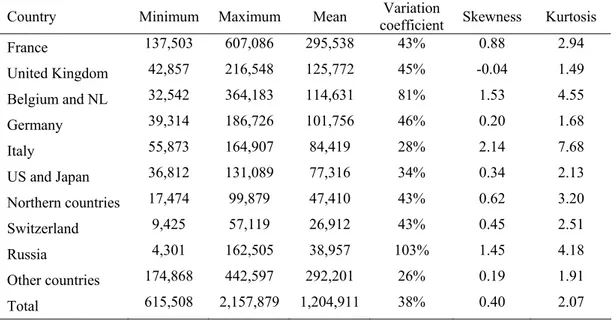
In this study we use the number of international tourist arrivals to Catalonia (first destination) over the period 2001:01 to 2012:07. Data is provided by the National Institute of Statistics (INE). Table 1 shows a descriptive analysis of tourist arrivals to Catalonia for the out-of-sample period (January 2009 to July 2012). Since data characteristics, including the origin of tourists, have an influence on the predictive ability of the models, we use tourist arrivals from all source markets. The first four visitor countries (France, the United Kingdom, Belgium and the Netherlands and Germany) account for more than half of the total number of tourist arrivals to Catalonia. Russia is the country that presents the highest dispersion in tourist arrivals, while Italy shows the highest levels of Skewness and Kurtosis.
Table 1. Descriptive analysis of tourist arrivals (levels)
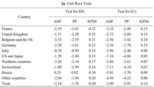
Before estimating the models, we determine whether the underlyingprocess which generated the series is stationary.If the series are found to have a unit root, differencing is necessary to obtain stationary series (Lim et al., 2009). In Table 2a
we present the results of several unit roots tests: the ADF test (Dickey and Fuller, 1979), the PP test (Phillips and Perron, 1988) and the KPSS test (Kwiatkowski et al., 1992) While the ADF and the PP statistics test the null hypothesis of a unit
root in yt, the KPSS statistic tests the null hypothesis of stationarity. In most countries we cannot reject the null hypothesis of a unit root at the 5% level. Similar results are obtained for the KPSS test, where the null hypothesis of stationarity is rejected in most cases. These results imply that differencing is required in most cases and prove the importance of detrending tourism demand data (Zhang and Qi, 2005). In order to eliminate both linear trends as well as seasonality we used the first differences of the natural log of tourist arrivals.
Table 2. Tests. Unit Root Tests and Unrestricted Cointegration Rank Tests
Given the common patterns displayed by most countries, we test for
cointegration using Johansen’s trace tests (Johansen, 1988, 1991). Trace statistics test the null hypothesis of r cointegrating vectors against the alternative
hypothesis of n cointegrating vectors. In Table 2b we present the results of five different unrestricted cointegration rank tests. It can be seen that we can only
reject the null hypothesis of nine cointegrating vectors with two of the tests. The fact that the evolution of tourist arrivals is multicointegrated has led us to apply a multivariate multiple-output neural network approach to obtain forecasts of tourism demand for all visitor markets.
4. Methodology
As the evolution of tourist arrivals from different visitor markets shows a common stochastic trend, we apply a multivariate neural network approach to obtain forecasts of tourism demand. To our knowledge this is the first study to evaluate the performance of different ANN models in a input multiple-output setting that uses the cross-correlations between the evolution of foreign visitors from different markets to a specific destination. This approach also allows to generate predictions for all visitors markets simultaneously without having to replicate the analysis for each country.
We divide the collected data into three sets: training, validation and test. This division is done in order to asses the performance of the network on unseen data (Bishop, 1995; Ripley, 1996). The initial size of the training set is determined to cover a five-year span in order to accurately train the networks. Therefore, the first sixty monthly observations (from January 2001 to January 2006) are selected as the initial training set, the next thirty-six (from January 2007 to January 2009) as the validation set, and the last 20% as the test set.
We implement an iterative forecasting scheme: after each forecast, a retraining is done by increasing the size of the set by one period and sliding the validation set by another period. This iterative process is repeated until the test set consists of the out-of-sample period. The selection criterion for the topology and the
parameters is the performance on the validation set. To ensure optimal parameter estimation, we apply a multi-start technique that initializes the neural network three times for different initial random values returning the best result. Using as a criterion the performance on the validation set, the results correspond to the selection of the best topology and the best spread in the case of the RBF neural networks.
Following the suggestions made by Koupriouchina et al. (2014), we evaluate
and 6 months ahead are generated in a recursive way. To assess the forecast accuracy we make use of three different measures. First, we compute the Root Mean Squared Error (RMSE). An additional key aspect that should be addressed is whether the reduction in RMSE is statistically significant when comparing models.
With this in mind, we obtain the measure of predictive accuracy proposed by Diebold and Mariano (1995). The DM loss-differential test for predictive accuracy tests the null hypothesis that the difference between the two competing series is non-significant. We calculate the DM test using a Newey-West type estimator to construct the t-statistic from a simple regression of the loss function on a constant. A negative sign of the t-statistic associated to the DM test implies that the
absolute value of the forecast error associated with the prediction coming from the competing series is lower, while a positive sign implies the opposite.
Finally, in order to attain a more comprehensive forecasting performance evaluation, we propose a dimensionless measure based on the CJ statistic for testing market efficiency (Cowles and Jones, 1937). This accuracy measure allows us to compare the forecasting performance between two competing models. This statistic consists on a ratio that calculates the proportion of periods in which the model under evaluation obtains a lower absolute forecasting error than the
benchmark model. In this study we use the no-change model as a benchmark. This new measure of forecast accuracy will be referred to as the percentage of periods with lower absolute error (PLAE).
Let us denote yt as actual value and yˆt as forecast at period t, t=1 K, ,n. Forecast errors can then be defined as et =yt −yˆt. Given two competing models A
and B, where A refers to the forecasting model under evaluation, whereas B stands for benchmark model, we can then obtain the proposed statistic as follows:
n λ PLAE n t t ∑ = =1 where ⎪⎩ ⎪ ⎨ ⎧ < = otherwise 0 if 1 t,A t,B t e e λ (4) 5. Results
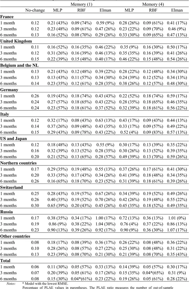
When analysing the forecast accuracy, MLP and RBF networks show lower RMSE values than Elman networks. Nevertheless, the no-change model outperforms both MLP and Elman networks. While RBF networks display the
lowest RMSE values for longer horizons in most countries, the no-change model shows higher percentages of PLAE than the rest of the networks, especially for the shorter forecasting horizons. The fact that the no-change model generates more accurate one-period-ahead forecasts than other more sophisticated models confirms previous research by Witt et al. (1994).
Table 3. Forecast accuracy. RMSE and percentage of PLAE (2010:04-2012:02)
When the forecasts are obtained incorporating additional lags of the time series, that is to say when the memory is set to three periods, the forecasting performance of RBF networks significantly improves in Switzerland and Russia for 6 months ahead. Nevertheless, the highest forecasting errors are always found in Russia. This result may be caused by the high dispersion observed in Russian tourist arrivals, and it endorses the conclusions obtained by Peng et al. (2014)
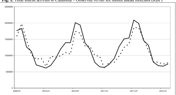
with reference to the fact that the country of origin affects the accuracy of the predictions. By contrast, the lowest RMSE value is obtained with the RBF network for total tourist arrivals, for 6 months ahead when the memory is zero, and for 3 months ahead when using a memory of three lags. In Fig.1 we compare the actual evolution of total tourist arrivals to the six moth ahead forecasts with RBF network.
Fig. 1. Total tourist arrivals to Catalonia – Observed versus six month ahead forecasts (RBF)
Unlike the results obtained by Chow (2003) when comparing the forecasting performance of Elman ANN to exponential smoothing and ARIMA models to forecast tourist arrivals to Hong Kong, we do not find evidence in favour of Elman networks, which suggests that divergence issues may arise when using dynamic networks with forecasting purposes. The only network that outperforms the benchmark model in most cases is the RBF. These results also show that hybrid models such as RBF, which combine supervised and non-supervised learning, are more indicated for tourism demand forecasting than models using supervised learning alone. Our finding on the suitability of using RBF ANNs for tourism demand forecasting in the hospitality industry confirms previous research by Cuhadar et al. (2014).
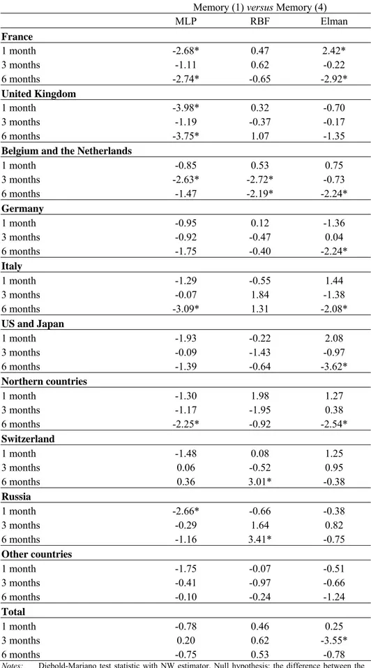
Finally, we repeat the analysis assuming different topologies regarding the memory values, which refer to the number of past months included in the context of the input, ranging from one to four months. Therefore, when the memory is one, the forecast is done using only the current value of the time series, without any additional temporal context. In Table 4 we present the results of the DM test so as to assess whether the different memory values are statistically significant on forecast accuracy. We find that in most cases, as the number of previous months used for concatenation increases, the forecasting performance of the different networks shows no significant improvement. This result suggests that the increase in the weight matrix is not compensated by the more complex specification, leading to overparametrization.
Table 4. Diebold-Mariano loss-differential test statistic for predictive accuracy
6. Conclusion
The increasing importance of the hospitality sector worldwide has led to a growing interest in new approaches to tourism demand forecasting. New methods provide more accurate estimations of anticipated tourist arrivals for effective managerial and policy planning. Artificial intelligence techniques are generating an increasing interest as a way to refine the predictions of tourist arrivals at the destination level. The main aim of this study is to develop a new forecasting framework to improve the forecasting performance of artificial neural networks. We use three models that represent alternative ways of handling information: the multi-layer perceptron, the radial basis function and the Elman recursive neural network.
6.1. Theoretical implications
The theoretical contribution of this study to the hospitality and tourism literature is twofold. On the one hand, we apply an innovative approach to improve the forecasting accuracy of artificial intelligence techniques. Based on multiple-input multiple-output structures, we design a framework that allows to incorporate the existing cross-correlations in tourist arrivals form different visitor
markets to a specific destination in neural networks. This new procedure allows to estimate the evolution of demand from all different markets simultaneously.
On the other hand, we propose a dimensionless forecasting accuracy measure based on the statistic for testing market efficiency. This new measure allows to compare the forecasting performance between two competing models by giving the percentage of periods in which the model under evaluation obtains a lower absolute forecasting error than the benchmark model.
By means of cointegration analysis we find that the evolution of arrivals from international visitor markets to Catalonia share a common trend, which leads us to apply a multivariate approach. The forecasting out-of-sample comparison shows that radial basis function models outperform the rest of the networks in most cases.
The research highlights that hybrid models, which combine supervised and non-supervised learning, are more indicated for tourism demand forecasting than models using supervised learning alone. Our results also suggest that when using dynamic or recurrent neural networks with forecasting purposes scaling issues may arise.
In order to evaluate the effect of the memory on the forecasting results, we repeat the analysis assuming different topologies regarding the number of lags used for concatenation and find no significant differences when additional lags are incorporated, especially in the case of multi-layer perceptron neural networks. This result can in part be explained by the cross-correlations accounted for in the multivariate approach.
6.2. Practical Implications
From a managerial perspective, the study provides a new and practical approach to predict the arrival of tourists, overnight stays or any other variable related to the daily activity of the hospitality and leisure industries. This new procedure allows practitioners to incorporate the common trends in customers from all markets in neural networks in order to anticipate the evolution of demand for all different markets simultaneously.
The study also provides managers with a new and easily interpretable measure to evaluate forecasts from different methods with the aim of attaining a more comprehensive forecasting performance evaluation.
The research reveals the suitability of hybrid models such as radial basis function networks for medium-term forecasts. The results of the analysis also highlight that the predictive performance can be improved by taking into account the connections between the different markets.
Demand is the most basic force driving the industry's development. Therefore, these findings aim to improve forecasting practices in the hospitality industry and provide new tools that may prove very helpful to anticipate future demand for planning purposes.
7. Limitations and future research
Nevertheless, this study is not without its limitations. First, a comparison between different tourist destinations would allow to analyze to what extent regional differences have a significant influence on forecasting accuracy. Another question to be considered in further research is whether a combination of the forecasts from different topologies may improve the accuracy of predictions. Finally, there is the question of whether the implementation of alternative
artificial intelligence techniques such as support vector regressions could improve the forecasting performance of neural networks.
References
Assaf, A.G., Barros, C.P. and Gil-Alana, L.A. (2011), “Persistence in the Short- and Long-Term Tourist Arrivals to Australia”, Journal of Travel Research, Vol. 50 No. 2, pp. 213-229.
Athanasopoulos, G. and de Silva, A. (2012), “Multivariate Exponential Smoothing for Forecasting Tourist Arrivals”, Journal of Travel Research, Vol. 51 No. 5, pp. 640-652.
Balaguer, J. and Cantavella-Jordá, M. (2002), “Tourism as a long-run economic growth factor: the Spanish case”, Applied Economics, Vol. 34 No. 3, pp. 877-884. Bishop, C.M. (1995), Neural networks for pattern recognition, Oxford University Press,
Broomhead, D.S. and Lowe, D. (1988), “Multi-variable functional interpolation and adaptive networks”, Complex Syst., Vol. 2, pp. 321-355.
Burger, C., Dohnal, M., Kathrada, M. and Law, R. (2001), “A practitioners guide to time-series methods for tourism demand forecasting: A case study for Durban, South Africa”, Tourism Management, Vol. 22 No. 4, pp. 403-409.
Cang, S. (2013), “A comparative analysis of three types of tourism demand forecasting models: individual, linear combination and non-linear combination”, International
Journal of Tourism Research, Vol. 15.
Capó, J., Riera, A. and Rosselló, J. (2007), “Tourism and long-term growth. A Spanish perspective”, Annals of Tourism Research, Vol. 34 No. 3, pp. 709-726.
Chen, K.Y. and Wang, C.H. (2007), “Support Vector Regression with Genetic
Algorithms in Forecasting Tourism Demand”, Tourism Management, Vol. 28 No. 1, pp. 215-226.
Cho, V. (2003), “A comparison of three different approaches to tourist arrival forecasting”, Tourism Management, Vol. 24 No. 3, pp. 323-330.
Claveria, O. and Datzira, J. (2010), “Forecasting tourism demand using consumer expectations”, Tourism Review, Vol. 65 No. 1, pp. 18-36.
Claveria, O. and Torra, S. (2014), “Forecasting tourism demand to Catalonia: Neural networks vs. time series models”, Economic Modelling, Vol. 36 No. 1, pp. 220-228.
Coleman, K.G., Graettinger, T.J. and Lawrence, W.F. (1991), “Neural networks for bankruptcy prediction: The power to solve financial problems”, AI Review, Vol. 5 July/August, pp. 48-50.
Cowles, A. and Jones, H. (1937), “Some A Posteriori Probabilities in Stock Market Action,” Econometrica, Vol. 5 No. 3, pp. 280-294.
Cuhadar, M., Cogurcu, I. and Kukrer, C. (2014), “Modelling and Forecasting Cruise Tourism Demand to İzmir by Different Artificial Neural Network Architectures”,
International Journal of Business and Social Research, Vol. 4 No. 3, pp. 12-28.
Dickey, D.A. and Fuller, W.A. (1979). “Distribution of the estimators for autoregressive time series with a unit root”, Journal of American Statistical Association, Vol. 74 No. 366, pp. 427-431.
Diebold, F.X. and Mariano, R. (1995), “Comparing predictive accuracy”, Journal of
Business and Economic Statistics, Vol. 13 No. 3, pp. 253-263.
Du Preez, J. and Witt, S.F. (2003), “Univariate versus Multivariate Time Series Forecasting: An Application to International Tourism Demand”, International
Journal of Forecasting, Vol. 19 No. 3, pp. 435-451.
Elman, J.L. (1990), “Finding structure in time”, Cognitive Science, Vol. 14, pp. 179-211. Goh, C., Law, R. and Mok, H.M. (2008), “Analyzing and Forecasting Tourism Demand:
Gounopoulos, D., Petmezas, D. and Santamaria, D. (2012), “Forecasting tourist arrivals in Greece and the impact of macroeconomic shocks from the countries of tourists’ origin”, Annals of Tourism Research, Vol. 39 No. 2, pp. 641-666.
Han, Z., Durbarry, R. and Sinclair, M.T. (2006), “Modelling US tourism demand for European destinations”, Tourism Management, Vol. 27 No. 1, pp. 1-10.
Haykin, S. (1999), Neural networks. A comprehensive foundation, Prentice Hall, New Jersey.
Huntley, D.G. (1991), “Neural nets: An approach to the forecasting of time series”, Social
Science Computer Review, Vol. 9 No. 1, pp. 27-38.
Johansen, S. (1988), “Statistical analysis of co-integration vectors”, Journal of Economic
Dynamics and Control, Vol. 12 No. 2-3, pp. 231-254.
Johansen, S. (1991), “Estimation and hypothesis testing of co-integration vectors in Gaussian vector autoregressive models”, Econometrica, Vol. 59 No. 6, pp. 1551-1580.
Kim, D. and Shwartz, Y. (2013), “The accuracy of tourism forecasting and data
characteristics: a meta-analytical approach”, Journal of Hospitality Marketing and
Management, Vol. 22 No. 4, pp. 349-374.
Kon, S.C. and Turner, W.L. (2005), “Neural network forecasting of tourism demand”,
Tourism Economics, Vol. 11 No. 3, pp. 301-328.
Koupriouchina, L., Van der Rest, J. and Schwartz. Z. (2014), “On revenue management and the use of occupancy forecasting error measures”, International Journal of
Hospitality Management, Vol. 41, pp. 104-114.
Kwiatkowski, D., Phillips, P.C.B., Schmidt, P. and Shin, Y. (1992), “Testing the null hypothesis of stationarity against the alternative of a unit root“, Journal of
Econometrics, Vol. 54 No. 1-3, pp. 159-178.
Law, R. (1998), “Room occupancy rate forecasting: A neural network approach”,
International Journal of Contemporary Hospitality Management, Vol. 10 No. 6,
pp. 234-239.
Law, R. (2000), “Back-propagation learning in improving the accuracy of neural
network-based tourism demand forecasting”, Tourism Management, Vol. 21 No. 4, pp. 331-340.
Law, R. (2001), “The impact of the Asian financial crisis on Japanese demand for travel to Hong Kong: a study of various forecasting techniques”, Journal of Travel &
Tourism Marketing, Vol. 10 No. 2-3, pp. 47-66.
Law, R. and Au, N. (1999), “A neural network model to forecast Japanese demand for travel to Hong Kong”, Tourism Management, Vol. 20 No. 3, pp. 89-97.
Lee, K.N. (2011), “Forecasting long-haul tourism demand for Hong Kong using error correction models”, Applied Economics, Vol. 43 No. 5, pp. 527-549.
Lim, C., Chang, C. and McAleer, M. (2009), “Forecasting h(m)otel guest nights in New Zeland”, International Journal of Hospitality Management, Vol. 28 No. 2, pp. 228-235.
MacKinnon, J.G., Haug, A. and Michelis, L. (1999), “Numerical Distribution Functions of Likelihood Ratio Tests for Cointegration”, Journal of Applied Econometrics, Vol. 14 No. 5, pp. 563-577.
Nam, K. and Schaefer, T. (1995), “Forecasting international airline passenger traffic using neural networks”, Logistics and Transportation, Vol. 31 No. 3, pp. 239-251. Ouerfelli, C. (2008), “Co-integration analysis of quarterly European tourism demand in
Tunisia”, Tourism Management, Vol. 29 No. 1, pp. 127-137.
Padhi, S.S. and Aggarwal, V. (2011), “Competitive revenue management for fixing quota and price of hotel commodities under uncertainty”, International Journal of
Hospitality Management, Vol. 30 No. 3, pp. 725-734.
Pai, P.F., Hong, W.C., Chang, P.T. and Chen, C.T. (2006), “The application of support vector machines to forecast tourist arrivals in Barbados: An empirical study”,
International Journal of Management, Vol. 23 No. 2, pp. 375-385.
Palmer, A., Montaño, J.J. and Sesé, A. (2006), “Designing an artificial neural network for forecasting tourism time-series”, Tourism Management, Vol. 27 No. 5, pp. 781-790.
Pattie, D.C. and Snyder, J. (1996), “Using a neural network to forecast visitor behavior”,
Annals of Tourism Research, Vol. 23 No. 1, pp. 151-164.
Peng, B., Song, H. and Crouch, G.I. (2014), “A meta-analysis of international tourism demand forecasting and implications for practice”, Tourism Management, Vol. 45, pp. 181-193.
Phillips, P.C.B. and Perron, P. (1988), “Testing for a unit root in time series regression”.
Biometrika, Vol. 75 No. 2, pp. 335-346.
Reynolds, D., Rahman, I. and Balinbin, W. (2013), “Econometric modeling of the US restaurant industry”, International Journal of Hospitality Management, Vol. 34, pp. 317-323.
Ripley, B.D. (1996), Pattern recognition and neural networks, Cambridge University Press, Cambridge.
Song, H. and Witt, S.F. (2006), “Forecasting international tourist flows to Macau”.
Tourism Management, Vol. 27 No. 2, pp. 214-224.
Song, H. and Li, G. (2008), “Tourism demand modelling and forecasting – a review of recent research”, Tourism Management, Vol. 29 No. 2, pp. 203-220.
Song, H., Li, G., Witt, S.F. and Athanasopoulos, G. (2011), “Forecasting tourist arrivals using time-varying parameter structural time series models”, International Journal
of Forecasting, Vol. 27 No. 3, pp. 855-869.
Talluri, K. and van Ryzin, G.J. (2002), “Revenue management under a general discrete choice model of consumer behavior”, Management Science, Vol. 50 No. 1, pp. 15-33.
Tsaur, S.H., Chiu, Y.C. and Huang, C.H. (2002), “Determinants of guest loyalty to international tourist hotels: a neural network approach”, Tourism Management, Vol. 23 No. 4, pp. 397-405.
Uysal, M. and El Roubi, M.S. (1999), “Artificial neural Networks versus multiple
regression in tourism demand analysis”, Journal of Travel Research, Vol. 38 No. 2, pp. 111-118.
Veloce, W. (2004), “Forecasting inbound Canadian tourism: an evaluation of error corrections model forecasts”, Tourism Economics, Vol. 10 No. 3, pp. 262-280. Witt, S.F., Witt, C.A. and Wilson, N. (1994), “Forecasting international tourists flows”,
Annals of Tourism Research, Vol. 21No. 3, pp. 612-628.
Yu, G. and Schwartz, Z. (2006), “Forecasting Short Time-Series Tourism Demand with Artificial Intelligence Models”, Journal of Travel Research, Vol. 45 No. 2, pp. 194-203.
Zhang, G., Putuwo, B.E. and Hu, M.Y. (1998), “Forecasting with artificial neural
networks: the state of the art”, International Journal of Forecasting, Vol. 14 No. 1, pp. 35-62.
Zhang, G.P. and Qi, M. (2005), “Neural network forecasting for seasonal and trend time series”, European Journal of Operational Research, Vol. 160 No. 2, pp. 501-514.
Table 1. Descriptive analysis of tourist arrivals (levels)
Country Minimum Maximum Mean coefficient Variation Skewness Kurtosis
France 137,503 607,086 295,538 43% 0.88 2.94 United Kingdom 42,857 216,548 125,772 45% -0.04 1.49 Belgium and NL 32,542 364,183 114,631 81% 1.53 4.55 Germany 39,314 186,726 101,756 46% 0.20 1.68 Italy 55,873 164,907 84,419 28% 2.14 7.68 US and Japan 36,812 131,089 77,316 34% 0.34 2.13 Northern countries 17,474 99,879 47,410 43% 0.62 3.20 Switzerland 9,425 57,119 26,912 43% 0.45 2.51 Russia 4,301 162,505 38,957 103% 1.45 4.18 Other countries 174,868 442,597 292,201 26% 0.19 1.91 Total 615,508 2,157,879 1,204,911 38% 0.40 2.07
Table 2. Tests. Unit Root Tests and Unrestricted Cointegration Rank Tests 2a. Unit Root Tests
Test for I(0) Test for I(1) Country
ADF PP KPSS ADF PP KPSS
France -2.19 -3.41 0.32 -3.32 -2.48 0.15
United Kingdom -1.71 -2.28 0.35 -2.72 -2.88 0.15
Belgium and the NL -3.53 -2.55 0.21 -2.56 -3.42 0.10
Germany -2.28 -3.61 0.23 -3.36 -3.70 0.15 Italy -0.78 -0.99 0.33 -3.96 -2.46 0.08 US and Japan -1.29 -2.40 0.33 -7.16 -4.06 0.03 Northern countries -3.26 -2.16 0.17 -3.86 -3.61 0.07 Switzerland -1.80 -2.99 0.16 -7.11 -4.10 0.07 Russia 0.25 0.82 0.30 -5.01 -3.70 0.09 Other countries -2.04 -1.96 0.20 -4.56 -4.23 0.06 Total -2.14 -1.76 0.30 -2.99 -2.91 0.14
2b. Unrestricted Cointegration Rank Tests
Type of test Assume no deterministic
trend in data
Allow for linear deterministic trend in data Allow for quadratic deterministic trend in data No intercept
in CE Intercept in CE Intercept in CE Intercept in CE Intercept and trend in CE Hypothesized
number of CE(s)
No test VAR No intercept in VAR Test VAR No trend in VAR Linear trend in VAR
0 : 0 r= H 856.6229 969.8334 946.8238 1085.223 1012.763 1 : 0 r≤ H 642.9016 741.4399 719.5322 857.7293 785.4048 2 : 0 r≤ H 489.0577 586.3624 566.5598 676.3885 604.4294 3 : 0 r≤ H 358.9547 452.6527 432.9569 541.7908 471.6636 4 : 0 r≤ H 267.2172 344.7378 327.2923 412.1319 342.0272 5 : 0 r≤ H 186.4016 256.9106 240.6405 314.3369 245.5905 6 : 0 r≤ H 118.7815 176.0951 162.8499 227.6863 160.0873 7 : 0 r≤ H 59.45009 110.2719 97.56685 149.9044 92.67206 8 : 0 r≤ H 20.81093 56.72323 47.79385 85.37519 38.75788 9 : 0 r≤ H 0.041106* (0.8681) 18.08417 10.98843 35.64879 0.944397* (0.3311)
Notes: Estimation period 2002:01-2012:07.
Tests for unit roots. Intercept included in test equation. Critical values for I(0) and I(1): ADF and PP tests - the 5% critical value is -2.88; KPSS test - the 5% critical value is 0.46.
Unrestricted Cointegration Rank Tests. * Denotes rejection of the hypothesis at the 0.05 level ** MacKinnon-Haug-Michelis p-values (MacKinnon et al., 1999). p-values in parentheses when different from zero.
Table 3. Forecast accuracy. RMSE and percentage of PLAE (2010:04-2012:02)
Memory (1) Memory (4)
No-change MLP RBF Elman MLP RBF Elman
France 1 month 0.12 0.21 (43%) 0.09 (74%) 0.59 (9%) 0.28 (26%) 0.09 (61%) 0.41 (17%) 3 months 0.12 0.23 (48%) 0.09 (61%) 0.47 (26%) 0.23 (22%) 0.09 (70%) 0.46 (9%) 6 months 0.13 0.16 (52%) 0.08 (70%) 0.29 (26%) 0.33 (30%) 0.09 (65%) 0.47 (13%) United Kingdom 1 month 0.11 0.16 (52%) 0.16 (35%) 0.46 (22%) 0.35 (9%) 0.16 (30%) 0.50 (17%) 3 months 0.12 0.31 (26%) 0.16 (39%) 0.46 (13%) 0.35 (35%) 0.16 (39%) 0.41 (26%) 6 months 0.15 0.22 (39%) 0.15 (48%) 0.40 (17%) 0.46 (22%) 0.15 (48%) 0.54 (26%)
Belgium and the NL
1 month 0.13 0.21 (43%) 0.12 (48%) 0.39 (22%) 0.28 (22%) 0.12 (48%) 0.34 (30%) 3 months 0.13 0.13 (43%) 0.11 (57%) 0.34 (30%) 0.24 (39%) 0.12 (52%) 0.34 (13%) 6 months 0.14 0.23 (35%) 0.12 (61%) 0.28 (35%) 0.38 (26%) 0.12 (57%) 0.48 (30%) Germany 1 month 0.26 0.19 (43%) 0.18 (74%) 0.43 (43%) 0.22 (52%) 0.18 (74%) 0.59 (17%) 3 months 0.24 0.27 (57%) 0.18 (65%) 0.43 (22%) 0.28 (35%) 0.18 (65%) 0.46 (35%) 6 months 0.24 0.23 (57%) 0.18 (61%) 0.37 (52%) 0.32 (39%) 0.18 (61%) 0.56 (22%) Italy 1 month 0.12 0.32 (17%) 0.08 (43%) 0.63 (13%) 0.43 (17%) 0.09 (43%) 0.44 (13%) 3 months 0.14 0.37 (26%) 0.09 (48%) 0.43 (35%) 0.33 (17%) 0.09 (57%) 0.49 (22%) 6 months 0.15 0.29 (43%) 0.09 (78%) 0.43 (22%) 0.52 (4%) 0.09 (83%) 0.57 (13%) US and Japan 1 month 0.12 0.18 (48%) 0.13 (43%) 0.55 (9%) 0.30 (17%) 0.13 (39%) 0.35 (22%) 3 months 0.16 0.32 (39%) 0.13 (52%) 0.28 (35%) 0.30 (26%) 0.13 (52%) 0.39 (35%) 6 months 0.20 0.21 (52%) 0.13 (65%) 0.28 (57%) 0.49 (39%) 0.13 (70%) 0.59 (26%) Northern countries 1 month 0.17 0.29 (35%) 0.19 (48%) 0.55 (13%) 0.37 (26%) 0.17 (61%) 0.41 (30%) 3 months 0.20 0.33 (35%) 0.17 (43%) 0.34 (26%) 0.41 (39%) 0.18 (48%) 0.34 (35%) 6 months 0.26 0.16 (65%) 0.18 (70%) 0.23 (52%) 0.31 (39%) 0.18 (61%) 0.39 (26%) Switzerland 1 month 0.25 0.28 (43%) 0.19 (57%) 0.67 (26%) 0.34 (39%) 0.19 (52%) 0.49 (26%) 3 months 0.26 0.40 (35%) 0.19 (52%) 0.70 (26%) 0.42 (26%) 0.19 (48%) 0.55 (22%) 6 months 0.30 0.65 (39%) 0.20 (43%) 0.45 (26%) 0.45 (35%) 0.18 (52%) 0.49 (35%) Russia 1 month 0.17 0.38 (35%) 0.34 (17%) 1.00 (17%) 0.72 (13%) 0.36 (13%) 1.01 (0%) 3 months 0.19 0.86 (9%) 0.38 (22%) 1.04 (30%) 0.76 (4%) 0.37 (22%) 0.86 (13%) 6 months 0.23 0.90 (13%) 0.39 (26%) 0.92 (17%) 0.90 (9%) 0.36 (30%) 1.07 (17%) Other countries 1 month 0.08 0.18 (17%) 0.08 (39%) 0.36 (17%) 0.26 (22%) 0.08 (48%) 0.36 (22%) 3 months 0.10 0.28 (26%) 0.08 (57%) 0.27 (22%) 0.25 (30%) 0.08 (48%) 0.31 (22%) 6 months 0.13 0.23 (39%) 0.08 (70%) 0.21 (30%) 0.21 (39%) 0.08 (70%) 0.35 (43%) Total 1 month 0.06 0.11 (30%) 0.05 (57%) 0.33 (13%) 0.14 (39%) 0.05 (57%) 0.30 (17%) 3 months 0.07 0.20 (39%) 0.05 (61%) 0.17 (26%) 0.15 (35%) 0.04*(65%) 0.31 (9%) 6 months 0.08 0.15 (30%) 0.04*(61%) 0.23 (22%) 0.19 (26%) 0.05 (61%) 0.28 (22%)
Notes: * Model with the lowest RMSE.
Percentage of PLAE values in parentheses. The PLAE ratio measures the number of out-of-sample periods with lower absolute errors than the benchmark model (no-change model).
Table 4. Diebold-Mariano loss-differential test statistic for predictive accuracy
Memory (1) versus Memory (4)
MLP RBF Elman France 1 month -2.68* 0.47 2.42* 3 months -1.11 0.62 -0.22 6 months -2.74* -0.65 -2.92* United Kingdom 1 month -3.98* 0.32 -0.70 3 months -1.19 -0.37 -0.17 6 months -3.75* 1.07 -1.35
Belgium and the Netherlands
1 month -0.85 0.53 0.75 3 months -2.63* -2.72* -0.73 6 months -1.47 -2.19* -2.24* Germany 1 month -0.95 0.12 -1.36 3 months -0.92 -0.47 0.04 6 months -1.75 -0.40 -2.24* Italy 1 month -1.29 -0.55 1.44 3 months -0.07 1.84 -1.38 6 months -3.09* 1.31 -2.08* US and Japan 1 month -1.93 -0.22 2.08 3 months -0.09 -1.43 -0.97 6 months -1.39 -0.64 -3.62* Northern countries 1 month -1.30 1.98 1.27 3 months -1.17 -1.95 0.38 6 months -2.25* -0.92 -2.54* Switzerland 1 month -1.48 0.08 1.25 3 months 0.06 -0.52 0.95 6 months 0.36 3.01* -0.38 Russia 1 month -2.66* -0.66 -0.38 3 months -0.29 1.64 0.82 6 months -1.16 3.41* -0.75 Other countries 1 month -1.75 -0.07 -0.51 3 months -0.41 -0.97 -0.66 6 months -0.10 -0.24 -1.24 Total 1 month -0.78 0.46 0.25 3 months 0.20 0.62 -3.55* 6 months -0.75 0.53 -0.78
Notes: Diebold-Mariano test statistic with NW estimator. Null hypothesis: the difference between the two competing series is non-significant. A negative sign of the statistic implies that the second model has bigger forecasting errors.
* Significant at the 5% level.
Fig. 1. Total tourist arrivals to Catalonia – Observed versus six month ahead forecasts (RBF) 0 500000 1000000 1500000 2000000 2500000 2009:07 2010:01 2010:07 2011:01 2011:07 2012:01
Notes: The black line represents the evolution of total tourist arrivals to Catalonia. The dotted line represents the 6 month ahead forecasts of total tourist arrivals to Catalonia obtained with the RBF model.