1
Title page
1
Article published in:
2
Regional Environmental Change, August 2018, Volume 18, Issue 6, pp 1765–1782. DOI:
3
https://doi.org/10.1007/s10113-018-1284-z 4
5
A landscape ecology assessment of land-use change on the Great
Plains-6Denver metropolitan edge (Colorado, USA; 1930-2010). Seeking sustainable
7farm systems in biodiversity maintenance
89
Joan Marul1a,*, Geoff Cunferb, Kenneth Sylvesterc, Enric Tellod 10
a Barcelona Institute of Regional and Metropolitan Studies, Autonomous University of Barcelona, 08193 11
Bellaterra, Spain 12
b Department of History, University of Saskatchewan, Saskatoon, SK S7N 5A5, Canada 13
c Inter-University Consortium for Political and Social Research. Institute for Social Research,University of 14
Michigan, Ann Arbor, MI 48106-1248, USA. 15
d Department of Economic History and Institutions, University of Barcelona, 08034 Barcelona, Spain 16 17 18 19 20 21 22 23 24 25 26 27 28
2
* Corresponding author: tel.:+34 93 5868880; fax: +34 93 5814433; email: [email protected] 29
3
Abstract
31
For better or worse, in those parts of the world with a widespread farming, livestock rising and 32
urban expansion, the maintenance of species richness and ecosystem services cannot depend only 33
upon protected natural sites. They have to rely on a network of cultural landscapes endowed with 34
their own associated biodiversity. This article presents a quantitative landscape ecology 35
assessment of land cover changes (1930-2010) experienced in a study area covering five Great 36
Plains counties in Colorado, adjacent to the northeastern edge of metropolitan Denver (USA). 37
Several landscape metrics assess the diversity of land cover patterns and their impact on the 38
dynamic processes of ecological connectivity. These metrics are applied to historical land cover 39
maps and datasets drawn from aerial photos and satellite imagery provided by the Great Plains 40
Population and Environment Project. The results emphasize the ecological functionality provided 41
by cropland-grassland mosaics that link the metropolitan edge with the surrounding habitats 42
sheltered in less human-disturbed areas, providing a heterogeneous land matrix able to maintain 43
bird species richness. The maps and indicators offer a general basis for selecting certain types of 44
landscape patterns and priority areas on which biodiversity conservation efforts and land use 45
planning can concentrate. They also suggest that keeping multifunctional farmland greenbelts 46
near the edge of metropolitan areas may provide important ecosystem services, supplementing 47
traditional conservation policies. 48
49
Keywords
50
Agro-ecosystems, land cover / land use change, ecological connectivity, landscape heterogeneity, 51
bird species richness, Great Plains. 52
4
1. Introduction
54 55
1.1. Can sustainable farm systems contribute to biodiversity conservation?
56
The loss of biodiversity is a focus of growing scientific and public concern (Schroter et al., 57
2005). The increasing impact of global land cover and land use change (LCLUC) challenges 58
scientific research to develop new approaches that can better inform public policies worldwide 59
(Turner et al. 2007). Landscape ecology provides useful quantitative tools for an environmental 60
assessment of the impacts of these LCLUC (Li, 2000), by studying the links between ecological 61
patterns and processes (Verburg et al., 2009). Landscape ecology metrics can also test ecological 62
models that identify land cover spatial heterogeneity and intermediate disturbances as 63
mechanisms explaining how complex-farming landscapes can generate and maintain biodiversity 64
(Marull et al., 2016). In this approach, land cover diversity of cultural landscapes differentiates 65
habitats and, in less disturbed patches, offers shelter to species endowed with a variety of dispersal 66
abilities that will attempt to recolonize the most disturbed lands (Loreau et al., 2010). 67
Our hypothesis is that large areas of cropland-pastureland mosaics could provide the kind of 68
heterogeneous cultural landscapes that may host an important associated biodiversity (Altieri, 69
1999). This wildlife-friendly farming (Tscharntke et al., 2012) would offer at the same time a 70
much needed ecological connectivity with less disturbed areas where other species can shelter 71
(Pino & Marull, 2012). The importance of heterogeneous landscapes for bird conservation is well 72
known (Boulinier, 2001), and many studies show that grassland bird populations have declined 73
throughout North America in recent decades (Brennan & Kuvlesky, 2005; Hamer et al., 2006). 74
The goal of this article is to analyze the effects of the LCLUC on the landscape ecological patterns 75
and processes that sustain bird species richness associated to cropland-grassland landscapes in 76
five Colorado counties linking northeast Denver’s metropolitan edge to the rural Great Plains 77
between 1930 and 2010. The impact of the study for land use policy and planning is the 78
assessment of the potential contribution of the Great Plain’s cropland-grassland mosaics as 79
multifunctional farmland green belts in the edge of metropolitan areas. 80
5
1.2. Socioecological transition and land cover change in the Great Plains, 1870-2010
82
Land cover has either a land mosaic or a gradient pattern (Forman, 1995). Gradients were an 83
outstanding feature of Great Plains grassland bioregions prior to Euro-American farm 84
colonization in the late nineteenth century. Far from being a pristine wilderness, the assemblage 85
of grasses and forbs were already cultural landscapes molded by Native Americans, mainly 86
through fire regimes that increased bison populations hunted on foot or on horseback (Pyne, 87
2001). Tallgrass, mixed grass and shortgrass bioregions assembled a variety of species largely 88
determined by rainfall gradients and soil capabilities, where bison grazing and prairie dog 89
foraging imprinted even greater patchiness at a small scale. Watercourses opened within this 90
grassland matrix some corridors of riparian vegetation, where Native Americans occasionally 91
seeded some crops and grew vegetable gardens (Hurt, 1987; Fenn, 2014). 92
Breaking the sod to begin widespread farming in the Great Plains entailed a strong socio-93
ecological transformation that caused a biodiversity decrease. Settlement devastated Native 94
American cultures, together with a large share of the bison population, and the government placed 95
both sets of survivors onto designated reserves (Cronon, 1992; Isenberg, 2000). The pioneer 96
methods of farming depleted soil fertility through a soil mining process over several decades that 97
only replenished small proportions of the nutrients extracted by crops (Burke et al., 2002; Cunfer 98
& Krausman, 2009)—a ‘metabolic rift’ (Fischer-Kowalski, 1998; Schneider & McMichael, 2010) 99
that released a high amount of greenhouse gas emissions (Parton et al., 2015). Yet Euro-American 100
settlers only plowed about 40% of the total land in the Great Plains during the pioneer era up to 101
the 1930s (Cunfer, 2005; Sylvester et al., 2016). By opening cropland patches within the 102
remaining grassland matrix, and by replacing bison with cow herds as grazers, they created 103
agroecosystems in a new cultural landscape. From then on, a key question for ecosystem services 104
provision is how much biodiversity can be kept associated to these agroecosystems. 105
The path towards several types of more mature and ecologically adapted mixed farming, 106
tightly integrated with animal husbandry or ranching, was suddenly interrupted in the Great Plains 107
by the extreme drought, dust storms and economic depression of the 1930s (Cunfer, 2005). The 108
succession of this unexpected environmental and socioeconomic crisis led to the implementation 109
6
of the Agricultural Adjustment Act in 1933 that launched an enduring era of public policies aimed 110
at soil conservation, cropland set-aside incentives, and farmers’ income stabilization through 111
credit and subsidies (Danbom, 1995; Rosenberg & Smith, 2009). As a result, cropland expansion 112
peaked in 1935 and has never returned to that level across the Great Plains. Farmers across the 113
United States as a whole withdrew over 16 million hectares of cropland from production each 114
year between 1936 and 1942. Efforts to reduce cropland were continued by the Soil Bank Program 115
from 1956 to 1972 and the Conservation Reserve Program from 1985 to 1996 (Sylvester et al., 116
2016). Yet the environmental and land use impacts of these cropland retirement or set-asided 117
policies are unclear, considering that they were combined with subsides meant to boost farmers’ 118
produce and incomes, and coincided with major technological changes in agriculture. 119
The twentieth century saw mechanization with diesel-powered tractors, synthetic fertilizers, 120
chemical pesticides, hybrid seeds of dwarf wheat and other grains, a new system of intensive 121
animal fattening with grain in feedlots, and the high-pressure irrigation pumps powered by 122
internal combustion engines and electric motors (Opie, 1993). All these changes in farm 123
management combined into a new industrial type of agriculture and livestock raising worldwide 124
known as the ‘green revolution’. Instead of pursuing and enhancing the agro-ecological 125
improvements evident prior to the 1930s, industrialization of agriculture meant a drastic change 126
of direction. From a land use standpoint the most salient feature was the new capability to bypass 127
former natural limits to which farmers had previously learned to adapt (Cunfer, 2005). 128
From the 1940s onwards crop diversity decreased across the Great Plains, while feedlots meant 129
livestock became less agro-ecologically integrated with the surrounding cropland and grassland. 130
Conversions from grassland to crops have been higher in the dry western shortgrass bioregion 131
than in the wetter eastern tallgrass zone, precisely because large unplowed areas remained there 132
up to the 1940s, when chemical fertilizers, irrigation and pesticides made them economically 133
feasible. The places with most land use change since the mid-twentieth century have been the 134
cropland-grassland mosaics located between high cropland areas and metropolitan regions, where 135
urban sprawl has encroached upon some of the best land, while farming and feedlots moved 136
towards poorer soils (Wu, 2000; Sylvester, 2016). 137
7
The general LCLUC patterns described fit well the trajectory of land use between 1930 and 138
the present in five counties of northeastern Colorado, near the edge of the Denver metropolitan 139
area. Besides localized and contrasting patterns of cropland intensification and grassland 140
preservation, the pressures of urban sprawl have also affected the near-metropolitan area. This 141
landscape ecology analysis of LCLUC applies landscape metrics that assess the structure and 142
functionality provided by cropland-grassland mosaics that linked different sides of the study area, 143
providing a land matrix able to maintain the associated biodiversity. After a brief presentation of 144
the study area and a description of the methods in section 2, we present the results in section 3. 145
First, land cover changes are detailed, then a number of landscape properties are analyzed and, 146
finally, the impact on birds’ species richness during the time frame is assessed. We discuss the 147
results in section 4 before presenting our conclusions. 148
149
2. Methods
150 151
2.1. Study area and main cartographic sources
152
This analysis of the LCLUC in 5 counties (Weld, Logan, Morgan, Adams and Arapahoe) near 153
Denver, Colorado (Fig. 1), relies on a large GIS database built from agricultural censuses with 154
detailed land use information collected from 1860-2007 at 22 time points by the Great Plains 155
Population and Environment Project (Gutmann, 2005). It aims to understand how changes in 156
farming and livestock raising affected ecological processes through the calculation of landscape 157
ecology indexes using this GIS database. The objective is to define consistent criteria and 158
guidelines to perform a Quantitative Landscape Ecology Assessment (QLEA) of this study area. 159
The land cover maps of the satellite scene (National Land Cover Database –NLCD; WRS path 160
33 row 32) used for the case study covers a large area of northern Colorado, reclassified for land 161
cover for 1992 and 2006 (Fig. 1). Within the satellite scene are 40 selected sample cells of 5x5 162
km (eight sites were randomly selected for each of the five counties considered). The aim of 163
making such selection is to create an analysis at nested scales, with data for one entire satellite 164
scene, for five counties within it, and for eight randomly selected sample cells within each county. 165
8
This case study (Fig. 2a) consists of analyzing the landscape ecology characteristics of 40 sample 166
cells within one satellite scene at five time points: 1930s, 1950s, 1970s, 1990s, and 2000s. For 167
each of these sample cells and time points this article presents three types of metrics: landscape 168
structure, landscape functionality, and land cover change (Table 1). 169
170
2.2. Landscape structure metrics
171
Five indicators of land cover diversity and fragmentation reveal the ecological landscape 172
patterns of the study area (Shannon, 1948; Jaeger, 2000) (Table A1). The Shannon Index (H) 173
assesses land cover equi-diversity. 174
H =
Σ
(Pi lnPi)175
where Pi is the proportion of land matrix occupied by each type of land cover.
176
The Largest Patch Index (LPI) reports the area of the largest polygon in each sample cell. 177
Polygon Density (PD) indicates the number of polygons in each sample cell. Edge Density (ED)
178
is the sum of the polygon perimeters in each sample cell. Effective Mesh Size (MESH) is the sum 179
of the areas of the polygons squared, divided by the size of the study area, an indicator that can 180
be interpreted as the inverse of landscape fragmentation. 181
MESH =
Σ
(Ai2) 1000 /Σ
(Ai)182
where Ai is the area of each polygon.
183 184
2.3. Landscape functionality metrics
185
Using the land cover map of the satellite scene at two time points, 1992 and 2006 (Fig. 1) it is 186
possible to calculate the Landscape Metric Index (LMI). The index is based on the landscape’s 187
structure capacity (as affected by human activities) to support organisms and ecological processes 188
(Table A1). This is calculated in a normalized range that moves from zero to ten on the basis of
189
four indicators: the capacity of relation between habitat patches, the ecotonic contrast between 190
adjacent habitats, the human impact on habitats, and the vertical complexity of habitats (see 191
Marull et al., 2007 for methodological details): 192
9
LMI = 1 + 9 (γi - γmin) / (γmax - γmin)
193
γ = I1+ I2+ I3+I4
194
where γi is the sum of the indicators for each polygon in the region, while γmin and γmax are the
195
minimum and maximum values, respectively. I1 is the potential relation, I2 is the ecotonic contrast,
196
I3 is the human impact, and I4 the vertical complexity.
197 I1 =
Σ
(Su si / Ku2 di2) 198 Ku =Σ
(ri Kh) 199 Kh = (H+P2) / 4 200 H = {0,1,2,3,4,5} 201 P = {0,1,2,3,4} 202where Su is the polygon area divided by the area of the satellite scene, si is the total affinity
203
areas, d is the distance between each polygon centroid and that of the rest, Ku is the landscape
204
characteristic dimension, Kh is the characteristic habitat dimension, H is the habitat hospitality,
205
and P is the vegetation size. 206 I2 =
Σ
(Cu Pc) / Pt 207 Cu = (Cf + Ce) / 2 208 Cf = {0, 1, 2, 3} 209 Ce = {0, 1, 2, 3} 210where Cu is the contrast between polygons, Pc is the perimeter of contact between polygons,
211
Pt is the total polygon perimeter, Cf is the physiognomic contrast, and Ce is the ecologic contrast.
212
I3 = Ku Pa/ Su
213
Pa= Pi+ Pd
214
where Pa is the perimeter of anthropogenic effect, Pi is the perimeter included, and Pd is the
215 adjacent perimeter. 216 I4 =
Σ
(ui Vi) 217 V = {0, 1, 2, 3, 4} 21810
u =
Σ
(ri Spi) / Su219
where V is the vertical structure, u is the habitat cover per polygon, and Spi is the polygon area
220
divided by the area of the satellite scene. 221
In order to calculate the Ecological Connectivity Index (ECI) the analysis changes scale, 222
moving from the entire satellite scene (Fig. 1) to also include the 40 randomly selected 5x5 km 223
sample cells nested within it (Fig. 2a). The index assesses the functionality of the land matrix 224
according to its ability to connect the horizontal flows of energy, matter, and information, which 225
sustain biodiversity (Table A1). The assessment of the evolving ecological connectivity (sensu 226
Lindenmayer & Fischer, 2007) for five time points is based in a simplification of the original 227
methodology proposed by Marull & Mallarach (2005). 228
The diagnosis of ecological connectivity relies on defining a set of Ecological Functional 229
Areas (EFA), which were considered the focal habitat patches to be connected, and a
230
computational model of cost-distance of displacement, which includes the effect of modelled 231
anthropogenic barriers (urban areas, infrastructures), considering the type of barrier, the range of 232
distances and the kind of land use involved. This analysis uses GIS to apply the model to available 233
historical land use maps comprising the satellite scene and the whole set of sample cells. As a 234
first step to calculate ECI all of the different land uses in each map (satellite scene and sample 235
cells) were reclassified into uniform landscapes. In order to establish the EFAs, the landscape 236
categories were grouped according to habitat ecological affinity and then analyzed 237
topologically—i.e. based on the criteria of minimum requirements and compactness indicated in 238
the literature (Andrén, 1994; Bender et al., 1998). In those landscape categories still unable to 239
generate simple EFAs another topological analysis generated cropland-grassland mosaics using 240
the same criteria described above. 241
The next step is to consider the anthropogenic barrier effects on landscape processes. An 242
impact analysis of the space surrounding each barrier (roads and built-up areas) relies on a 243
weighted classification of landscape polygons that act as barriers to ecological connectivity. The 244
algorithm is based on a computational model of cost-distance in displacements, which includes a 245
11
weight for each type of barrier and a potential matrix of land uses affected. The model applies the 246
CostDistance function in ArcGIS software and uses two databases: a ‘source’ surface for each
247
type of barrier (XBs; s = 1 ... 5) and an ‘impedance’ surface from the potential matrix of areas
248
affected (XA). This process results in a ‘cost-distance adapted’ measure (d’s = bs – ds; where bs –
249
ds > 0; being ds the cost-distance). Assuming that the effect of a barrier in YS point of the
250
surrounding space is logarithmic, and decreases as a function of the distance (Kaule, 1997), we 251
have: 252
YS = bs – ks1 ln [ks2 (bs – d’s) + 1]
253
where bs is the weight of each barrier, ks1 and ks2 are constants (adapting the graph to the
254
distribution obtained using empirical data) and d’s is the cost-distance adapted for each barrier.
255
The barrier effect Y is defined as the sum of effects of all types and the cartographic expression 256
obtained as a result is a surface: 257
Y =
Σ
Ys258
The algorithm used to determine the ecological connectivity between landscape units applies 259
a computational model of cost-distance, which considers the different classes of EFAs to connect 260
and an impedance surface of land that includes a matrix of potential affinity, together with the 261
effect of anthropogenic barriers. Again the model applies the CostDistance function using two 262
databases: a ‘source’ surface for each type of EFA (XC'r; r = 1 ... 3) and an ‘impedance’ surface
263
resulting from applying the effects of barriers to the potential affinity matrix (XI = XC'r + XY). The
264
result is a cost-distance adapted to each type of functional ecological area (with d’r <20,000 to
265
avoid irrelevant information or concealment of results). By calculating the value of the sums of 266
cost-distances adapted, this computational model of ecological connectivity defines a Basic 267
Ecological Connectivity Index (ECIb) in a normalized range that varies from zero to ten. This ECIb
268
emphasizes the role played by the land matrix: 269
ECIb = 10 – 9 [ln (1 + xi) / ln (1 + xt )3]
270
where xi is the value of the sum of the cost-distance by pixel and xt the maximum theoretical
271
cost distance. 272
12 Then ECIa is the Absolute Ecological Connectivity Index:
273
ECIa =
Σ
ECIb / m274
where m is the absolute number of EFAs considered. This indicator emphasizes the role played 275
by all sorts of agricultural and cropland-grassland mosaics in maintaining ecological connectivity 276
(Pino & Marull, 2012). 277
278
2.4. Land cover change metrics
279
Three indicators reveal the nature of land cover change over time (Table A1). The Land Use 280
Change (LUC) indicator measures the cell average of the land use change of each pixel (Table 1), 281
distinguishing between no change (0) and change (1). The resulting LUC score reveals three 282
stability regimes: stable (LUC = 0-0.2), semi-stable (LUC = 0.2-0.4), and non-stable (LUC = 0.4-283
1). Pressure (P) measures the percentage of pixels that change to urban or agriculture land use 284
for each cell: no change (0); total change (1). Agriculture pressure Pa: low (Pa = 0-0.25); medium 285
(Pa = 0.0.25-0.5); high (Pa = 0.5-0.75); very high (Pa = 0.75-1). Urban pressure Pu: low (Pu =
0-286
0.05); medium (Pu = 0.05-0.1); high (Pu = 0.1-0.2); very high (Pu = 0.2-1). Naturalness (N)
287
measures the degree of preservation of grassland habitats. Five N levels are possible: grasslands 288
(5), shelterbelts (4), pastures (3), crops and recently mowed areas (2), and urban areas, roads, and 289 railways (1). 290 291 2.5. In search of bio-indicators 292
Is there a link between landscape heterogeneity and biodiversity change? To test that 293
possibility, this study employs as a first attempt of empirical underpinning the North American 294
Breeding Bird Survey (BBS) data that provides bird observations from six driving routes within 295
the study area. The BBS is an annual roadside survey of birds seen and heard along rural roads 296
and secondary highways distributed throughout North America. Only the six BBS routes that fall 297
within the satellite image scene from northern Colorado are used here (Fig. 2b). An expert who 298
records all birds heard or seen within a 4-km buffer zone of the road has surveyed each of these 299
13
routes annually in June since 1967. Data are summarized as a list of species reported on five stops 300
along the route (Sauer et al., 2008). The 5 stops allow assembling the observations of the total 301
number of bird species, and the specifically grassland bird species. BBS data come from 1991 302
and 2007 because they are the two time points with a larger sample, that broadly correspond with 303
1992 and 2006 satellite image land cover data (given that annual land cover change is practically 304
undetectable on this scale). 305
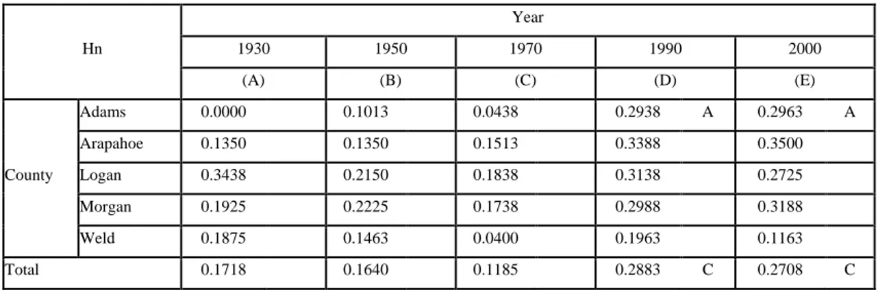
The landscape structure of the study area has been analyzed from a raster generated by the 306
National Land Cover Database (NLCD) using multispectral TM images obtained by Landsat 5 307
during 1992 and 2006 (section 2.1). Eight different land cover types are classified: water, urban, 308
neutral (unproductive), forest, scrub, grassland/herbaceous, pasture/hay and croplands. These 309
land cover maps have been used to calculate landscape heterogeneity (H). This study then 310
compares the effects of land cover spatial distribution on local species richness of all birds (555 311
species), and of specifically grassland birds (27 species). The six BBS driving routes have been 312
overlaid on the 30 x 30 m2 resolution indices’ maps to extract 4 km buffers around each route. 313
Farmland-associated biodiversity is much more than only birds. Yet, birds have some useful 314
features as an indicator of the general quality of a farm environment. Many of them feed on 315
insects, seeds and fruits, and sometimes also on earthworms, snails and slugs, small reptiles and 316
mammals. In turn, small birds are also hunted by raptors. Their presence as predators and prey 317
indicates the abundance of many other species upon which they depend. Birds can easily fly from 318
less disturbed land to more disturbed landscape units where they find trophic resources. Finally, 319
their populations have been better monitored than any other taxon. Hence bird observation data 320
in the Denver study area can be used as a bio-indicator, and help us to bear out whether the 321
ecological landscape metrics used are an artefact, or whether they reflect actual values of 322
landscape patterns and ecological processes. Yet, it must be acknowledged that the results of this 323
empirical check can only be indicative, not conclusive. 324
325
3. Results
326 327
14
3.1. Land cover change results
328
The mosaic of crops amidst a grassland land matrix characterizes the predominant land cover 329
pattern of the Great Plains. The satellite scenes mainly show a general decrease in grassland and 330
an increase in cropland and urban areas in north-eastern Colorado between 1992 and 2006 (Fig.
331
3a), given that urban sprawl has tended to move the agricultural ring surrounding the metropolitan 332
area further away (Sylvester et al., 2013). Conversely, the sample cell analysis based on aerial 333
photograph interpretation (Fig. 3b) indicates a decline in cropland and increase in grassland cover 334
on a wider scale during the last period of analysis (1990s-2000s), as the authors confirmed in 335
fieldwork. The signature of plowing the land remains visible for a long time in air photo time 336
series of these more distant areas (Sylvester & Rupley 2012). There is a homogenization of 337
grasses during the recovery phase when croplands are abandoned or put into conservation reserve 338
programs—since the disturbance signal is still visible in the lack of heterogeneity in the 339
reflectance values of the satellite imagery (Maxwell & Sylvester, 2012). The recovery of 340
grassland vegetation in aerial photo imagery is less immediate than the multispectral signature 341
visible in satellite imagery. Aerial photo interpretation can detect tillage in semi-arid grasslands 342
for up to 50 years after cropland abandonment (McGinnies et al., 1991). 343
Due to the opposite trends experienced in the cropland ring nearer to Denver metropolitan 344
edge and the more distant cropland-grassland into the Great Plains, some counties had very 345
different land use regimes (Fig. 4). The land use change identified as LUCr indicates a change to
346
urban and agricultural land uses. That identified as LUCp indicates a change to grassland land
347
uses. The land cover change carried out was more towards the former than the latter, except 348
between the 1930s and 1950s (Table 1)—although changes depend on the scale of observation. 349
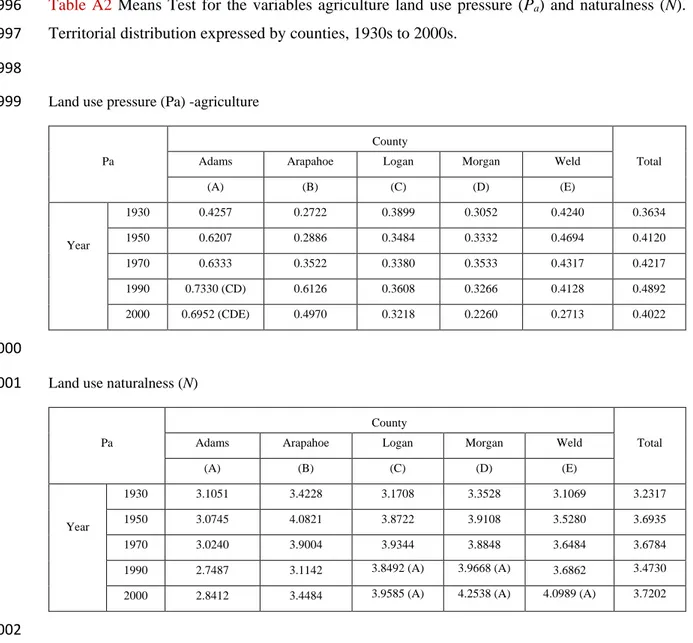
The land use pressure is high for agriculture (Pa) and low for urban uses (Pu) because sample cells
350
are located mainly in non-urban areas (Table 1). In general, pressure (Pa) increased in the period
351
analyzed throughout the agricultural ring surrounding the metropolitan area, and that fact 352
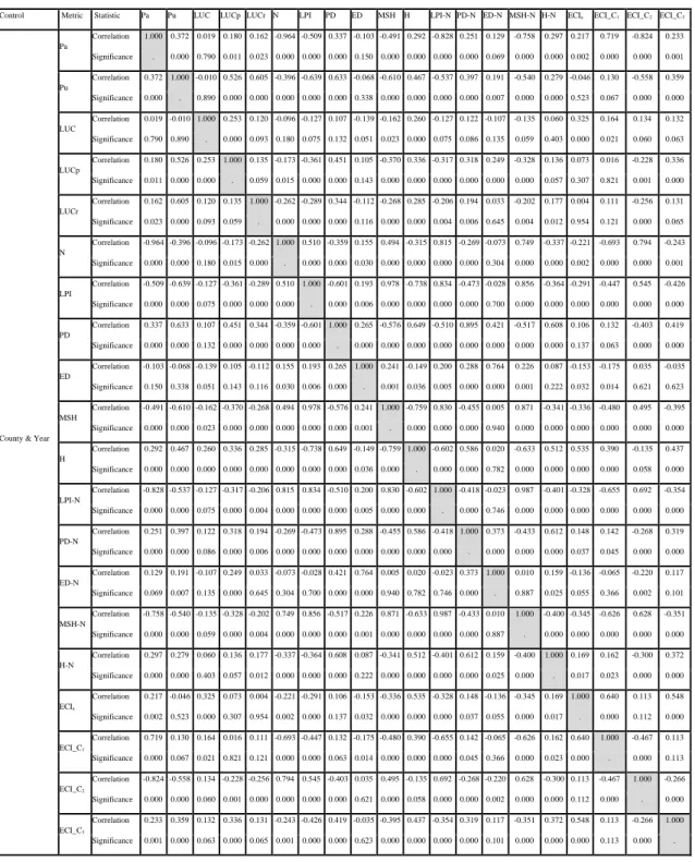
coincides with a decrease in the habitats preserved in less disturbed land covers (N) (Table A2). 353
This is clearly revealed by the strong correlation between both variables (-0.964; Table 3). It is 354
15
also important to note the significant statistical differences between time points, considering 355
counties, albeit with a small sample size. 356
357
3.2. Landscape structure results
358
LPI measures the largest polygon in each cell as an indicator of the grain thickness of the
359
landscape. LPI decreased in the period of analysis, mainly in grassland categories (Table 1). ED 360
measures the total length of perimeters of the polygons of each land cover, in relation to the 361
surface area of the cell. ED indicates the potential exchanges between land covers/land uses. The 362
landscape ecotony changed in the period analyzed, with noticeably higher levels in the 1950s 363
(Table 1). PD measures the number of polygons as a very simple indicator of the smaller or larger
364
grain size of patches. In general, there were not important changes in PD values. MESH is the 365
inverse of the extent of this fragmentation, related to a lower grain size. There was an increase in 366
landscape fragmentation in less human-disturbed categories such as grassland (Fig. 4). H 367
measures land cover equi-diversity, and it did not change, only revealing an increase in grassland 368
categories (Table 1). At the same time, land cover fragmentation (inverse of MESH) increased 369
with time, at a rate equal to land cover diversity (Table A3). This change is revealed by the 370
correlation between both variables (-0.759; Table 3). The ecological connectivity index (ECI) 371
reveals how different land uses (H) are ecologically well-connected within the landscape in a 372
mosaic structure (ED), rather than in a fragmented and unconnected pattern of land uses (MESH) 373
because of the presence of barriers such as roads or urban areas (Table 3). 374
375
3.3. Landscape functionality results
376
The satellite scene analysis shows a decrease in the functional attributes of the landscape 377
between 1992 and 2006, clearly assessed by the LMI as a measure of the capacity to maintain 378
ecological processes and biodiversity associated to human-modified landscapes (Fig. 5a), which 379
according to land cover distributions seem to have been mainly caused by urban development and 380
intensification of agriculture (Table 2). There was also a decrease in landscape connectivity (Fig.
381
5b), mainly located near urban areas. The size, topology and mosaic structure of the EFAs 382
16
influence connectivity, and riparian corridors become very important in fragmented landscapes. 383
Habitats tended to remain isolated from the rest of the land matrix due to the growing effect of 384
anthropogenic barriers created around the metropolitan area. 385
This study also adjusts the methodology according to the criteria and the constants that must 386
be incorporated into a QLEA to analyze, for each sample cell, the historical land cover change 387
between 1938 and 2006 in the study area. For each random cell an ECIb average value of different
388
patterns is calculated. The results show interesting correlations between the landscape change and 389
landscape structure metrics used (with differences between the five counties and also between 390
years) and their influence on the QLEA (Table 3). Correlation analysis reveals the existence of 391
different ECIb behaviors in the agro-ecosystems analyzed (ECI1 (agriculture), ECI2 (grassland),
392
ECI3 (cropland-grassland mosaic), and ECIa (all categories). The results make apparent the
393
importance of agriculture and cropland-grassland mosaics in jointly maintaining ecological 394
connectivity (ECIa) of the study area.
395 396
3.4. Biodiversity results
397
The total number of birds observed declined significantly (P<0.001) between 1967 and 2007 398
along routes located within the satellite scene (Fig. 6a), while the number of species increased 399
between 1967 and 1990, but decreased thereafter (Fig. 6b). As only stops along the route that 400
match in all years have been used to obtain this dataset, the results can only suggest some trends 401
that require further research. The decrease in bird observations occurred after cropland (as 402
measured in the sample cells) reached its greatest extent in the 1990s (Fig. 3b). Focusing only on 403
the period between 1991 and 2007, just after the turning point described above, there was a 404
decrease in the number of birds (Fig. 6a) and species (Fig. 6b) observed. 405
Thus, there seems to be a positive correlation between landscape heterogeneity and bird 406
species observations (Fig. 7a). Along the survey routes, the percentage of cropland-grassland 407
mosaic decreased, despite the introduction of grassland conservation policies. The dominant 408
habitat corresponded to a cropland-grassland mosaic along five routes, and cropland along one 409
route, for 1991. In 2007 three routes had a cropland-grassland mosaic as the dominant habitat, 410
17
cropland in two routes, and urban in one route. Even if the small number of observations precludes 411
any statistical significance for these results (P>0.05), the hints are interesting. In those routes 412
where the dominant land cover changed to intensified cropland and urban covers, the number of 413
species and individuals observed decreased. The number of different land cover categories and 414
the landscape heterogeneity also increased between 1991 and 2007 for all routes. Grassland bird 415
species were more common in homogeneous landscapes (Fig. 7b), whereas the number of all 416
kinds of bird species increased in heterogeneous cropland-grassland landscapes as measured by 417
higher H’ values (Fig. 7a). Yet we also found a differentiated effect depending on the percentage 418
of grassland (P<0.05; Fig. 8a) and cropland (P>0.05; Fig. 8b), in accordance with the habitat 419
needs of particular species. 420
421
4. Discussion
422
A multi-scalar analysis of a land cover dataset from the 1930s to the 2000s (Fig. 3) reveals a 423
much more complex and dynamic pattern of LCLUC than the aggregated figures accounted only 424
at a regional level (Hartman et al., 2011; Sylvester et al., 2013). Together with conversion of 425
cropland to grassland, there have been many opposite trends experienced in grassland located in 426
marginal soils formerly considered unsuitable to plow (Sylvester & Rupley, 2012). In some parts 427
of the Great Plains, cultivation of poor soils has exceeded 1930s levels over the last seventy years. 428
These land use shifts in and out of cultivation can only be detected by zooming down to local 429
scales, as we have done in our study areas (Fleischner 1994; Christian & Wilson, 1999; Samson 430
et al., 2004; Knopf & Samson, 2013; Freese et al., 2014). 431
Grassland and cropland were the dominant land covers in 1992 (Fig. 3). However, a general 432
loss of agricultural land cover during the next years to urban expansion, scrub, and forest reflected 433
a combination of agricultural land use conversion for social, economic or conservation reasons— 434
e.g. participation in government incentives for farmers to convert highly erodible cropland to 435
protective grassland cover. The grassland areas un-cropped and endowed with high species 436
richness are only a fraction of the overall land matrix, and have become increasingly isolated 437
amidst cropland-grassland mosaics (Fig. 5). For better or worse, a great deal of the species 438
18
richness maintained at the bioregional scale depends on managed patches within cultural 439
landscapes. Studying the LCLUC patterns from a landscape ecology standpoint provides useful 440
information to assess when, where and why such cropland-grassland mosaics provide habitat 441
differentiation that can be enhanced or reduced. 442
The results suggest a positive association between bird species richness and landscape 443
heterogeneity, which deserves a deeper study in future addressed to test the hypothesis that bird 444
species richness tends to be lower in more homogeneous landscapes than in heterogeneous ones— 445
except when specific grassland bird species are considered. These results indicate that rural 446
cropland-grassland mosaics may provide farm-associated habitats and ecological connectivity 447
that support a wider range of bird species richness (Bock et al., 1999). Finally, increasing urban 448
sprawl and transport infrastructures lead to decrease in ecological connectivity (Fig. 5 and Table
449
2). If farmlands and agro-pastoral mosaics are important contributors to habitat differentiation, 450
and ecological connectors, this assessment and its associated maps provide useful information to 451
identify critical points and priority areas for a land use planning aimed at enhancing the ecosystem 452
services that biodiversity provides in metropolitan areas (Dupras et al., 2016). 453
According to the well-known patch-corridor-matrix model (Forman, 1995), agricultural 454
colonization meant an increase in land cover heterogeneity. New cropland-grassland mosaics 455
replaced the previous continuous gradients in grassland diversity (see section 1.2). This 456
combination of a spatially uneven disturbance with greater land cover heterogeneity could offer 457
more differentiated habitats to various species and ecological communities. As a result, β-458
diversity (species richness at landscape scale) increased, overriding the inevitable fall in α-459
diversity (at plot level) within plowed cropland—which is the typical impact of agroecosystem 460
functioning on its own associated biodiversity (Gliessmann, 2006). 461
Agroecosystem functioning always involves an energy interchange between farmers and 462
natural systems (Tello et al., 2016). Through this interchange, farmers accumulate information 463
and turn it into site-specific knowledge that orients the ecological disturbances they exert to create 464
specific land use patterns that give rise to cultural landscapes (Marull et al., 2016). From a 465
landscape ecology standpoint, the emergence in the Great Plains of increasingly integrated and 466
19
complex agroecosystems, regionally adapted and differentiated, meant the consolidation of a 467
diversity of land mosaics by 1930 (section 1.2). These cultural landscapes can still allow some 468
degree of biodiversity maintenance (Tscharntke et al., 2005), by providing heterogeneous agro-469
ecological and pastoral land covers well connected with the differentiated habitats kept in less 470
disturbed landscape patches (Agnoletti, 2014). 471
The results highlight the key role played by cropland-grassland mosaics in maintaining the 472
ecological functionality of the edge environments between the Great Plains and Denver 473
metropolitan fringes (Fig. 5). They can provide a heterogeneous but permeable land matrix able 474
to offer many habitats and a great deal of interconnectivity required to maintain an associated 475
biodiversity, particularly once this biodiversity is no longer identified with wilderness (Cronon, 476
1996). We are talking of a biodiversity needed to provide vital ecosystem services to farmers and 477
society at large, not comparable with the one that existed in the grasslands before the Great Plains 478
agricultural colonization. These are no longer pristine natural areas, but rather cultural mosaics 479
created by the land use management performed by past agricultural systems until the advent of 480
intensive industrial agriculture in mid-twentieth century (section 1.2). 481
Now these landscape mosaics are under pressure in the Denver area because of the combined 482
effect of three ongoing land use changes: urban sprawl, industrial agriculture, and cropland 483
retirement linked to subsidy programs. Biodiversity is at risk especially due to the decrease in 484
land cover diversity and ecotones, as well as in viable ecological connectors. Further research, 485
with more empirical data form different taxon is needed, to confirm or reject our hypothesis that 486
cropland-pastureland mosaics can provide green infrastructures to maintain ecological processes 487
and biodiversity near metropolitan areas of the Great Plains. 488
489
Policy implications
490
Several lessons can be learned from this landscape ecology assessment of land use changes in 491
the study area, with important implications for landscape and urban planning. First, land use 492
policy must consider the territory as a whole, taking into consideration the role of cropland-493
grassland mosaics in keeping a relevant degree of associated biodiversity. Only safeguarding 494
20
National Parks and other protected areas that remain isolated in very far away locations is not 495
enough to ensure the biodiversity-related ecosystem services that farmers, and society at large, 496
require—pollination, pest and disease control, soil fertility maintenance, detoxification, water 497
cleaning, and recreational (Millennial Ecosystem Assessment, 2005). 498
Second, in human-managed landscapes a cropland-grassland mosaic can provide an agro-499
ecological matrix able to nurture biological diversity—e.g. plant communities that retain native 500
species; bees, butterflies and other insects that perform a vital role as pollinators; many birds, and 501
small mammals like prairie dogs whose burrows improve degraded soils and become a prey for 502
carnivores such as the black-footed ferret, swift fox, golden eagle, American badger and 503
ferruginous hawk (Miller at al., 2000; Freemark et al., 2003; Lindsay et al., 2013). These managed 504
cropland-grassland mosaics can also provide ecological connectivity to the natural habitats 505
sheltered in less disturbed sites, sometimes linking them up to some protected areas. 506
Third, the combination of the role played by cropland-grassland mosaics (measured by H’) as 507
provider of habitats for farm-associated biodiversity, and as ecological connectors (measured by 508
ECI) to avoid isolation between habitats, can contribute to biological conservation. Land use and
509
agricultural policies jointly addressed to develop wildlife-friendly ways of farming and livestock 510
grazing may reinforce natural protection policy, establishing a land sharing approach to 511
conservation that can reinforce the land sparing effort in creating National Parks (Fischer at al., 512
2008; Phalan et al., 2011). Such an approach would include avoiding urban sprawl and 513
counteracting with corrective measures the barrier effect on ecological connectivity exerted by 514
linear transport infrastructures. 515
Farm subsidies, mainly addressed thus far at sustaining farmers’ income and avoiding soil 516
erosion, can also take into account these broader aims. Conservation policy must explicitly 517
recognize the human-dominated nature of agricultural landscape mosaics and actively promote 518
the design of biodiverse landscape features, edge habitats, and corridors of connectivity across 519
heterogeneous land matrices that will extend up to natural spaces. Citizens, urban dwellers and 520
politicians should understand that behind aesthetic farm landscapes there are farmers who deserve 521
to earn a fair income for their labor while managing and protecting spaces that provide many 522
21
types of ecosystem services that become increasingly valuable near metropolitan areas. Finally, 523
by providing a long-term, dynamic perspective, the environmental history of the Great Plains 524
landscape may also help to raise society’s awareness in order to adopt a broader approach to the 525
sustainability of ecosystem services provision (Millennial Ecosystem Assessment, 2005). 526
527
5. Conclusions
528
In the metropolitan fringes of the Great Plains wilderness is gone, and is not going to come 529
back. Nature protected areas do not exist in a size and distance that matters in our study area of 530
Denver, and are unlikely to be established in future. This means that both people and nature live 531
in human-dominated landscapes. The relevant question now is how much biodiversity can remain 532
associated to the cropland-grassland mosaics of these cultural landscapes, so as to provide the 533
vital ecosystem services that farmers and urban dwellers require. 534
It is widely recognized that at a global scale industrialization of agriculture with the Green 535
Revolution adopted from the mid-twentieth century onwards has been a major driver of 536
biodiversity loss (Matson et al., 1997; Tilman et al., 2002). At the same time, it is increasingly 537
evident that well-managed agroecosystems can play a key role in biodiversity maintenance 538
(Bengtsson et al., 2003; Tscharntke et al., 2005) by providing complex landscape well-connected 539
mosaics that can maintain a relevant degree of species richness (Tress et al., 2001; Jackson et al., 540
2007). Depending on land use intensities and the type of farming, agricultural systems may either 541
enhance or decrease this biodiversity associated to cultural landscapes (Swift et al., 2004). 542
The results obtained by applying landscape ecology metrics to the LCLUC in the area 543
northeast of Denver (Colorado, USA) confirm this twofold effect of farm systems on land cover 544
heterogeneity capable of hosting bird species richness. They suggest that keeping more 545
sustainable farm management may benefit and improve the biodiversity maintenance enhanced 546
by grassland conservation policies. On the one hand, grassland and pastureland patches have to 547
be preserved from the extension of intensified cropland along the farmland belt around the 548
metropolitan edge in order to avoid monocultures and keep a heterogeneous mosaic free from 549
landscape fragmentation and barrier effects that jeopardize ecological connectivity. On the other 550
22
hand, in more distant areas where pastures are growing at the expense of cropland abandonment, 551
a mosaic pattern can be maintained and improved by closer integration between the two land uses 552
and extensive ranching. 553
These results are relevant for a better understanding of how the biodiversity associated to 554
cultural landscapes is affected by agricultural intensification, urban sprawl, and transport 555
infrastructure, as well as grassland recovery in retired former farmland. The main impact of the 556
study for landscape and urban planning is the possible application of cropland-grassland mosaics 557
as green belts in Great Plains–metropolitan edges. This combination of positive and negative 558
impacts of farming on biodiversity raises an interesting question for further research: How can 559
the great technological divide of the Green Revolution, and its ability to surpass climate and 560
ecological limits, be reconciled with the apparent long-term permanence of land use patterns in 561
the Great Plains, where the peak plow-up of about 40% of the total surface for cropland, reached 562
in the 1930s, has never been surpassed? 563
23
References
565
Agnoletti, M. (2014). Rural landscape, nature conservation and culture: some notes on research 566
trends and management approaches from a (southern) European perspective. Landscape and 567
Urban Planning 126, 66-73.
568
Altieri, M. (1999). The ecological role of biodiversity in agroecosystems. Agriculture Ecosystems 569
and Environment 74, 19-3.
570
Andrén, H. (1994). Effects of habitat fragmentation on birds and mammals in landscapes with 571
different proportions of suitable habitat: a review. Oikos 71, 355–366. 572
Bender, D. J., Contreras, T. A., & Fahrig, L. (1998). Habitat loss and population decline: a meta-573
analysis of the patch size effect. Ecology 79, 517–533. 574
Bengtsson, J., Angelstam, P., Elmqvist, T., Emanuelsson, U., Folke, C., Ihse, M., Moberg, F. & 575
Nyström, M. (2003). Reserves, Resilience and Dynamic Landscapes. Ambio 32 (6), 389-396. 576
Bock, C. E., Bock, J. H., & Bennett, B. C. (1999). Songbird abundance in grasslands at a suburban 577
interface on the Colorado high plains. Studies in Avian Biology 19, 131-6. 578
Boulinier, T., Nichols, J. D, Hines, J. E., Sauer, J. R., Flather, C. H., & Pollock, K. H. (1998). 579
Higher temporal variability of forest breeding bird communities in fragmented landscapes. 580
Proc. Natl. Acad. Sci. 95, 7497-7501.
581
Brennan, L. A., & Kuvlesky, W. P. (2005). North American grassland birds: an unfolding 582
conservation crisis? Journal of Wildlife Management 69, 1-13. 583
Christian, J. M., & Wilson, S. D. (1999). Long-term ecosystem impacts of an introduced grass in 584
the northern Great Plains. Ecology 80, 2397–2407. 585
Cronon, W. (1992). A place for stories: Nature, history, and narrative. The Journal of American 586
History 78(4), 1347-1376.
587
Cronon, W. (1996). The Trouble with Wilderness: Or, Getting Back to the Wrong Nature. 588
Environmental History 1(1), 7-28.
589
Cunfer, G. (2005). On the Great Plains: Agriculture and Environment. College Station: Texas A 590
& M University Press. 292 pp. 591
24
Cunfer, G., & Krausmann, F. (2009). Sustaining Soil Fertility: Agricultural Practice in the Old 592
and New Worlds. Global Environment 4, 8-47. 593
Cunfer, G., & Krausmann, F. (2012). Sustaining Agricultural Systems in the Old and New World: 594
A Long-Term Socio-Ecological Comparison. In Long Term Socio-Ecological Research: 595
Studies in Society-Nature Interactions Across Spatial and Temporal Scales, ed. Simron Jit 596
Singh, Helmut Haberl, Marian Chertow, Michael Mirtl, and Martin Schmid. Berlin: Springer, 597
269-296. 598
Cunfer, G., & Krausmann, F. (2016). Adaptation on an agricultural frontier: Socio-ecological 599
profiles of Great Plains settlement, 1870-1940. Journal of Interdisciplinary History. XLVI (3), 600
355-392. 601
Danbom, D. B. (1995). Born in the Country: A History of Rural America. Baltimore: Johns 602
Hopkins University Press. 306 pp. 603
Dupras, J., Marull, J., Parcerisas, Ll., Coll, F., Gonzalez, A., & Tello, E. (2016). The impacts of 604
urban sprawl on ecological connectivity in the Montreal Metropolitan Region. Environmental 605
Science and Policy 58, 61-73.
606
Fenn, E. A. (2014). Encounters at the Heart of the World: A History of the Mandan People. New 607
York: Hill & Wang. 456 pp. 608
Fischer, J., Brosi, B., Daily, G. C., Ehrlich, P. R., Goldman, R., Goldstein, J., Lindenmayer, D. 609
B., Manning, A. D., Mooney, H. A., Pejchar, L., Ranganathan, J. & Tallis, H. (2008). Should 610
agricultural policies encourage land sparing or wildlife-friendly farming? Front Ecol Environ 611
6 (7), 380-385. 612
Fischer, J., & Lindenmayer, D.B. (2007). Landscape modification and habitat fragmentation: 613
a synthesis. Global Ecological Biogeography 216, 265-280. 614
Fischer-Kowalski, M. (1998). Society’s Metabolism. The Intellectual History of Materials Flow 615
Analysis, Part I, 1860-1970. Journal of Industrial Ecology 2(1), 61-136. 616
Fleischner, T. L. (19949. Ecological costs of livestock grazing in western North America. 617
Conservation Biology 8 (3), 629-644.
25
Forman, R. T. T. (1995). Land Mosaics. The Ecology of Landscapes and Regions. Cambridge 619
University Press, Cambridge. 620
Freemark, K. E., Boutin, C. & Keedy, C., J. (2003). Importance of Farmland Habitats for 621
Conservation of Plant Species. Conservation Biology 16(2), 399-412. 622
Freese, C. H., Fuhlendorf, S. D., & Kunkel, K. (2014). A Management Framework for the 623
Transition from Livestock Production toward Biodiversity Conservation on Great Plains 624
Rangelands. Ecological Restoration 32, 358-68. 625
Gilbert-Norton, L., Wilson, R., Stevens, J. R., Beard, K. H. (2010). A meta-analytic review of 626
corridor effectiveness. Conservation Biology 24, 660-668. 627
Gliessman, S. R. (ed) (1990). Agroecology: researching the ecological basis for sustainable 628
agriculture. Springer, New York. 629
Gutmann, M. P. (2005). Great Plains Population and Environment Data. Ann Arbor: Inter-630
university Consortium for Political and Social Research. 631
Hamer, T. L., Flather, C. H., & Noon, B. R. (2006). Factors associated with grassland bird species 632
richness: the relative roles of grassland area, landscape structure, and prey. Landscape Ecology 633
21, 569-583. 634
Hartman, M. D., Merchant, E. R., Parton, W. J., Gutmann, M. P., Lutz, S. M., & Williams, S. A. 635
(2011). Impact of Historical Land Use Changes in the U.S. Great Plains, 1883 to 2003. 636
Ecological Applications 21(4), 1105-1119.
637
Hurt, R. D. (1987). Indian Agriculture in America. Lawrence: University Press of Kansas. 290 638
pp. 639
Isenberg, A. C. (2000). The Destruction of the Bison: An Environmental History, 1750-1920. 640
Cambridge University Press. New York. 206 pp. 641
Jackson, L. E., Pascual, U., & Hodgkin, T. (2007). Utilizing and conserving agrobiodiversityin 642
agricultural landscapes. Agriculture Ecosystems and Environment 121 (3), 196-210 643
Jaeger, J. A. G. (2000). Landscape division, splitting index, and effective mesh size: new 644
measures of landscape fragmentation. Landscape Ecology 15, 115-130. 645
26
Kaule, G. (1997). Principles for mitigation of habitat fragmentation. In Canters (Ed.), Proceedings 646
of the International Conference on Habitat Fragmentation, Infrastructures and the Roles of 647
Ecological Engineering. Maastricht and The Hague, The Netherlands, September 1995, 17– 648
21. 649
Knopf, F. L., & Samson, F. B. (2013). Ecology and Conservation of Great Plains Vertebrates. 650
Vol. 125: Springer Science & Business Media. 651
Li, B-L. (2000). Why is the holistic approach becoming so important in landscape ecology? 652
Landscape and Urban Planning 50, 27-41.
653
Lindenmayer, D. B., & Fischer, J. (2007). Tackling the habitat fragmentation panchreston. TREE 654
22, 127-132. 655
Lindsay, K. E., Kirk, D. A., Bergin, T. M., Best, L. B., Sifneos, J. C. & Smith, J. (2013). Farmland 656
Heterogeneity Benefits Birds in American Mid-west Watersheds. The American Midland 657
Naturalist 170(1), 121-143.
658
Loreau, M., Mouquet, N. & Gonzalez, A. (2010). Biodiversity as spatial insurance in 659
heterogeneous landscapes. P. Natl. Acad. Sci. 100 (22), 12765-12770. 660
Marull, J., & Mallarach, J. M. (2005). A new GIS methodology for assessing and predicting 661
landscape and ecological connectivity: Applications to the Metropolitan Area of Barcelona 662
(Catalonia, Spain). Landscape and Urban Planning 71, 243-62. 663
Marull, J., Pino, J., Mallarach, J. M., & Cordobilla, M. J. (2007). A land suitability index for 664
strategic environmental assessment in metropolitan areas. Landscape and Urban Planning 81, 665
200-12. 666
Marull, J., Font, C., Tello, E., Fullana, N., Domene, E., Pons, M., & Galán, E. (2016). Towards 667
an energy–landscape integrated analysis? Exploring the links between socio-metabolic 668
disturbance and landscape ecology performance (Mallorca, Spain, 1956–2011). Landscape 669
Ecology 31, 317-336.
670
Matson, P. A, Parton, W. J., Power, A. G. & Swift, M. J. (1997). Agricultural Intensification and 671
Ecosystem Properties. Science 277, 504-509. 672
27
McGinnies, W. J., Shantz H. L., & McGinnies W. G. (1991). Changes in Vegetation and Land 673
Use in Eastern Colorado: A Photographic Study, 1904 to 1986. Agricultural Research Service,
674
ARS-85, Springfield, VA: U.S. Department of Agriculture. 675
Maxwell, S.K., & Sylvester K.M. (2012). Identification of ever and never cropped land (1984-676
2010) using Landsat and Maximum NDVI image composites: Southwestern Kansas case 677
study. Remote Sensing of the Environment 121, 186-195. 678
Millennial Ecosystem Assessment (2005). Ecosystems and Human Well-Being. Island Press, 679
Washington, DC. 680
Miller, B., Reading, R., Hoogland, J., Clark, T., Ceballos, G., List, R., Forrest, S., Hanbury, L., 681
Manzano, P., Pacheco, J. & Uresk, D. (2000). The Role of Prairie Dogs as a Keystone Species: 682
Response to Stapp. Conservation Biology 14(1), 318-321. 683
Opdam, P., Steingröver, E., & van Rooij, S. (2006). Ecological networks. A spatial concept for 684
multi-actor planning of sustainable landscapes. Landscape and Urban Planning 75, 322–332. 685
Opie, J. (1993). Ogallala: Water for a Dry Land. Lincoln: University of Nebraska Press. 412 pp. 686
Parton, W. J., Gutmann, M. P., Merchant, E. R., Hartman, M. D., Adler, P. R., McNeal, F. M., & 687
Lutz, S. M. (2015). Measuring and Mitigating Agricultural Greenhouse Gas Production in the 688
Us Great Plains, 1870–2000. Proceedings of the National Academy of Sciences 112, E4681-689
E88. 690
Phalan, B., Onial, M., Balmford, A. & Green, R. E. (2011). Reconciling Food Production and 691
Biodiversity Conservation: Land Sharing and Land Sparing Compared. Science 333, 1289-692
1291. 693
Pino, J., Rodà, F., Ribas, J., & Pons, X. (2000). Landscape structure and bird species richness: 694
implications for conservation in rural areas between natural parks. Landscape and Urban 695
Planning 49, 35-48.
696
Pino, J., & Marull, J. (2012). Ecological networks: Are they enough for connectivity 697
conservation? A case study in the Barcelona Metropolitan Region (NE Spain). Land Use 698
Policy 29, 684-90.
28
Rosenberg, N. J., Smith, S. J. (2009). A sustainable biomass industry for the North American 700
Great Plains. Environmental Sustainability 1, 121–132. 701
Pyne, S. J. (2001). Fire: A Brief History. Seattle: University of Washington Press. 204 pp. 702
Samson, F. B., Knopf, F. L., & Ostlie, W. R. (2004). Great Plains ecosystems: past, present, and 703
future. Wildlife Society Bulletin 32 (1), 6–15. 704
Sauer, J. R., Hines, J. E., Fallon, J. (2008). The North American Breeding Bird Survey, Results 705
and Analysis 1966–2007. Version 5.15. 2008. USGS Patuxent Wildlife Research Center, 706
Laurel, Maryland, USA. 707
Schneider, M., McMichael, P. (2010). Deepening, and repairing, the metabolic rift. J. Peasant 708
Stud. 37, 461-484. 709
Schröter, D., Cramer, W., Leemans, R., Prentice, I. C., Araújo, M. B., Arnell, N. W., Bondeau, 710
A., Bugmann, H., Carter, T. R., Gracia, C. A., de la Vega-Leinert, A. C., Erhard, M., Ewert, 711
F., Glendining, M., House, J. I., Kankaanpää, S., Klein, R. J., Lavorel, S., Lindner, M., 712
Metzger, M. J., Meyer, J., Mitchell, T. D., Reginster, I., Rounsevell, M., Sabaté, S., Sitch, S., 713
Smith, B., Smith, J., Smith, P., Sykes, M. T., Thonicke, K., Thuiller, W., Tuck, G., Zaehle, S., 714
& Zierl, B. (2005). Ecosystem service supply and vulnerability to global change in Europe. 715
Science 310, 1333-7.
716
Shannon, C. E., 1948. A Mathematical Theory of Communication. The Bell System Technical 717
Journal 27. 379-423, 623-656.
718
Swift, M. J., Izac, A. M. N., & van Noordwijk, M. (2004). Biodiversity and ecosystem services 719
in agricultural landscapes—are we asking the right questions? Agriculture Ecosystems and 720
Environment 104 (1), 113-134.
721
Sylvester, K. M., Brown, D. G., Deane, G. D., & Kornak, R. N. (2013). Land transitions in the 722
American plains: Multilevel modeling of drivers of grassland conversion (1956-2006). 723
Agriculture, Ecosystems and Environment 168, 7-15.
724
Sylvester, K. M. Gutmann, M. P., & Brown D. G. (2016). At the Margins: Agriculture, Subsidies 725
and the Shifting Fate of North America’s Native Grassland. Population and Environment 37 726
(3), 362-390. 727
29
Sylvester, K. M., & Rupley, E. S. A. (2012). Revising the Dust Bowl: High Above the Kansas 728
Grasslands. Environmental History 17: 603-633. 729
Tello, E., Galán, E., Sacristán, V., Cunfer, G., Guzmán, G. I., González de Molina, M., 730
Krausmann, F., Gingrich, S., Padró, R., Marco, I., & Moreno-Delgado, D. (2016). Open-ing 731
the black box of energy throughputs in agroecosystems: a decompositionanalysis of final 732
EROI into its internal and external returns (the Vallès County Cat-alonia, c.1860 and 1999). 733
Ecological Economics 121, 160-174.
734
Tilman, D. (2002). The Ecological Consequences of Changes in Biodiversity. A Search for 735
General Principles. Ecology 80 (5), 1455-1474. 736
Tress, B., Tress, G., Décamps, H. & d’Hauteserre, A. M. (2001). Bridging human and natural 737
sciences in landscape research. Landscape and Urban Planning 57, 137-41. 738
Tscharntke, T., Klein, A. M., Kruess, A., Steffan-Dewenter, I., & Carsten Thies, C. (2005). 739
Landscape perspectives on agricultural intensification and biodiversity-ecosystem service 740
management. Ecological Letters 8, 857-874. 741
Tscharntke, T., Clough, Y., Wanger, T. C., Jackson, L., Motzke, I., Perfecto, I., Vandermeer, J. 742
& Whitbread, A. (2012). Global food security, biodiversity conservation and the future of 743
agricultural intensification. Biological Conservation 151, 53-59. 744
Turner, B. L., Lambin, E. F., Reenberg, A. (2007). The emergence of land change science for 745
global environmental change and sustainability. Proc Natl Acad Sci 104 (52), 20666–20671. 746
Verburg, P. H., van de Steeg, J., Veldkamp, A., & Willemen, L. (20099. From land cover change 747
to land function dynamics: a major challenge to improve land characterization. Journal of 748
Environmental Management 90, 1327-1335.
749
Wrbka, T., Erb, K.-H., Schulz, N. B., Peterseil, J., Hahn, Ch., & Haberl, H. (2004). Linking 750
pattern and process in cultural landscapes. An empirical study based on spatially explicit 751
indicators. Land Use Policy 21, 289-306. 752
Wu, J. (2000). Slippage Effects of the Conservation Reserve Program. American Journal of 753
Agricultural Economics 82, 979-92.
754 755
30
Table 1 Application of land use change and landscape structure metrics in the sample cells at five
756
time points, 1930s to 2000s. 757
758
Land use change 759 760 Landscape structure 761 a) Total categories 762 Code Indicator 1930s 1950s 1970s 1990s 2000s
LPI Largest Patch Index (km2)
915 967 1028 929 960
ED Edge Density (km) 57 77 64 65 69
PD Polygon Density (nº) 55 59 40 45 52
MESH Effective Mesh Size (km2)
6.36 6.90 7.56 6.69 6.82
H Shannon Index 1.03 0.96 0.92 0.93 0.91
b) No urban categories (agriculture and grassland)
763
Code Indicator 1930s 1950s 1970s 1990s 2000s
LPI Largest Patch Index (km2)
915 967 1028 929 960
ED Edge Density (km) 39 60 46 46 55
PD Polygon Density (nº) 38 41 28 30 36
MESH Effective Mesh Size (km2)
6.47 6.98 7.63 6.77 6.90
H Shannon Index 0.88 0.81 0.80 0.86 0.84
c) Less disturbed categories (grassland alone)
764
Code Indicator 1930s 1950s 1970s 1990s 2000s
LPI Largest Patch Index (km2)
871 853 840 692 784
ED Edge Density (km) 55 86 61 57 69
PD Polygon Density (nº) 24 24 19 21 26
MESH Effective Mesh Size (km2)
7.20 7.20 7.09 5.60 6.20
H Shannon Index 0.17 0.16 0.12 0.29 0.27
765
Note: The results show the average of all the sample cells (N=40).
766
Code Indicator 1930 -1950s 1950 -1970s 1970 -1990s 1990 -2000s 1930 -2000s
LUC Land Use Change 0.225 0.134 0.164 0.135 0.358
LUCr
Land Use Change
regressive 0.004 0.007 0.005 0.006 0.012
LUCp
Land Use Change
progressive 0.008 0.003 0.003 0.002 0.006
Code Indicator 1930s 1950s 1970s 1990s 2000s
Pu Urban pressure 0.011 0.014 0.012 0.014 0.018
Pa Agriculture pressure 0.363 0.412 0.421 0.489 0.402