Spectral Classified Vector Quantization (SCVQ) for Multispectral Images

UNIVERSITY

OF TRENTO

DEPARTMENT OF INFORMATION AND COMMUNICATION TECHNOLOGY

38050 Povo – Trento (Italy), Via Sommarive 14

http://www.dit.unitn.it

SPECTRAL CLASSIFIED VECTOR QUANTIZATION (SCVQ)

FOR MULTISPECTRAL IMAGES

Luigi Atzori

and

F. G. B. De Natale

January 2002

S

PECTRAL

C

LASSIFIED

V

ECTOR

Q

UANTIZATION

(SCVQ)

FOR

M

ULTISPECTRAL

I

MAGES

Luigi Atzori

1*

, Member, IEEE and Francesco G.B. De Natale

2

, Member, IEEE

1

DIEE - University of Cagliari, P.zza D’Armi – 09123 Cagliari, Italy e-mail: gigi@diee.unica.it, phone: +39 070 675 5902, fax: +39 070 675 5900

2

DIT - University of Trento, Via Mesiano, 77 – 38050 Trento, Italy e-mail: denatale@ing.unitn.it, phone: +39 0461 882671, fax: +39 0461 882672

Abstract

Multi- and hyper-spectral data pose severe problems in terms of storage capacity and transmission

bandwidth. Although recommendable, compression techniques require efficient approaches to

guarantee an adequate fidelity level. In particular, depending on the final destination of the data, it

could be necessary to maximize several parameters, as for instance the visual quality of the

rendered data, the correctness of their interpretation, or the performance of their classification.

Based on the idea of Spectral Vector Quantization, the approach proposed in this paper aims at

combining a compression and a classification methodology into a single scheme, in which visual

distortion and classification accuracy can be balanced a-priori according to the requirements of

the target application. Experimental results demonstrate that the proposed approach can be

employed successfully in a wide range of application domains.

Keywords: Multispectral image compression, Vector Quantization, Classification

EDICS: 1-OTHA

A preliminary version of this work was presented at the IEEE International Geoscience and Remote

Sensing Symposium 2000, Honolulu, 24-28 July 2000

1. Introduction

In the past years, due to the increase in the spatial and spectral resolution of remote sensing devices, data compression is becoming a need both on-board (for efficient downlinks) and on-ground (for long-term storage). In particular, multi- and hyper-spectral images pose severe storage and transmission problems due to the huge amount of data associated to a single shot. Several studies have been directed towards the development of efficient techniques that should be capable of achieving a good trade-off between bitrate reduction and quality preservation. Unfortunately, the term ‘quality’ does not only refer to the visual appearance of data as in classical picture coding applications, but it usually involves more complex aspects related to the performance of successive processing steps. As a matter of fact, the spectral signature of an

image pixel often represents the most important information in many remote sensing applications, for it allows to discriminate among different targets in data analysis procedures. Despite this, most of the techniques currently adopted in remote sensing data compression directly mimic the corresponding photographic image coding approaches, thus focusing on visual distortion minimization and disregarding the possible impact of compression on the performance of automatic processing tools. For instance, the impact of compression can affect a cascade data analysis module or an automatic classifier negatively.

In order to achieve data compression, coding techniques applied to optical remotely-sensed data take advantage of the presence of two redundancy sources: spatial correlation among neighboring pixels in the same spectral band, and spectral correlation among different bands at the same spatial location. Several strategies can be adopted to separately or jointly exploit these sources of redundancy, but a cascade of spectral and spatial decorrelation is usually preferred, as in the case of three dimensional transform coding [1], which is based on the combination of two transforms that successively exploit inter- and intra-band correlation. The Kahrunen-Loeve Transform (KLT) is usually preferred as a first step, due to its signal energy compaction capability, while for the second step, the Discrete Cosine Transform has been widely studied, also on account of its important role in international standards. In particular, the JPEG standard can be successfully applied to intra-band coding, since it can heavily compress the less significant image planes generated by the KLT (i.e., those associated to smaller eigenvalues) with a negligible visual distortion. These planes are in fact characterized by very low dynamics, and their number usually increases with the number of bands, thus making the use of 3D transform coding attractive in high spectral-resolution imagery.

Approaches based on baseline Vector Quantization (VQ) [2], which show the advantage of simple hardware and software decoding, though associated to a relatively high image distortion, have long been investigated [3, 4]. It is to be pointed out that their efficiency strictly depends on the codebook characteristics: in particular, the use of adaptive codebooks that can be updated according to the image characteristics can produce good results at the expense of a higher complexity.

The problem of combining compression and classification using a VQ approach has a long history. Classical solutions consist of an independent design for Vector Quantizer and classifier [5], with each step using a different optimality criterion, the former being based on MSE, while the latter on Bayesian risk minimization. More recently, various approaches have been proposed, mostly based on a clustering of the codebook, in which the VQ is explicitly designed to work as a classifier, almost ignoring the compression aspect [6-8]. One of the most common approaches to clustered VQ is Learning VQ (LVQ) [9, 10], where the encoder selects the codeword on the basis of MSE minimization, while codebook generation is performed attempting to limit classification error.

In [11], the problem is investigated with particular reference to the case of hyperspectral images. The proposed technique, which is based on a Spectral Vector Quantization (SVQ), performs a quantization of the multidimensional space associated to the spectral components of image pixels. The codebook is thus generated by clustering the feature space and selecting a prototype signature for each cluster.

In this work, an alternative scheme, which combines image compression and supervised classification into a single step, is presented. It therefore achieves excellent classification performance at the expense of moderate visual quality worsening. In section 2, SVQ is briefly reviewed as a basis of the proposed approach. Thus, in the following sections the principles of the proposed technique are described in detail, the experimental analysis reported, and the conclusions finally drawn.

2. Spectral Vector Quantization (SVQ)

In Fig.1 a block scheme of a SVQ codec is depicted: for each pixel pi to be encoded, the spectral signature is compared to the M codevectors and associated to the nearest one according to a given distance criterion. Only a sequence of codevector addresses is then transmitted to the decoder, which replaces the original pixel with the quantized signature, operating as a simple look-up table. As to codebook generation, different

strategies can be adopted: Kohonen’s Self Organizing Features Map (SOFM) is often considered a good solution, for it achieves an efficient codebook organization in terms of entropy minimization.

The compression factor CFSVQ attained by SVQ can easily be computed on the basis of the number of vectors

M in the codebook, the number of spectral bands N, and the number of bits originally associated to each band

(here supposed equal for all bands, for the sake of simplicity), namely:

M

b

N

CF

_SVQ 2

log

⋅

=

(1)

Compared to other techniques, SVQ presents notable advantages in terms of compression capability and reconstruction quality. From the viewpoint of compression performance, Eq. 1 highlights the fact that the efficiency of SVQ increases proportionally to the number of spectral bands, making it particularly suited to hyper-spectral images. As to the resulting image quality, it can be observed that the distortion introduced by the encoding procedure independently affects single pixels, resulting in a very low visual impact and a total absence of tiling artifacts, typical of block coding techniques (e.g., spatial VQ or block transform coding techniques).

Several experiments have been carried out in order to test the efficiency of SVQ on various data sets with different characteristics. The two image sets referred to in the following results are “Feltwell” and “Blue-bury”. The former consists of six visible spectral bands of a rural area in UK, acquired by Airborne TM sensors, which represent an area containing only agricultural fields, human constructions (roads, buildings, etc.) being totally absent. The latter consists of nine spectral bands, six of which in the visible portion of the electromagnetic spectrum, and three in the infrared portion (near, middle -near, and middle infrared). The encompassed land portion includes human constructions (roads, walls, houses, and other structures) as well as rural areas. In both images the intensity of each original spectral component was coded at 8 bits per pixel. The two datasets were also provided with the relevant ground truth, with a number of known classes of 5 and 9, respectively.

In Fig. 2, a detail of a spectral band of the “Feltwell” dataset is shown (2.a), and compared with the same details co-decoded with SVQ and JPEG, respectively (2.b-c). The size of the VQ codebook was set to M=64, thus yielding CFSVQ=8; the JPEG quality parameter was set so as to obtain the same compression factor. It can be observed that SVQ produces more appreciable results in terms of perceptive distortion, for it

preserves the definition of fine details better and provides a more satisfying visual quality of the decoded image. Fig. 3 shows a set of charts, which shows the global impact of compression on average spectral signatures with reference to the nine classes of the “Blue-bury” dataset. For each class, the average spectral signatures calculated on the original and SVQ compressed images are compared. Also in this example the codebook size was set to M=64, although the compression factor is higher (CFSVQ=12) than the previous example due to the larger number of spectral bands. Apparently, only minor variations affect the spectral signatures of most classes. Nevertheless, it is to be pointed out that this average measure does not allow to appreciate the internal variation within a class, which can be very important in the classification phase. Moreover, it disregards the local error associated to small areas or even single points. This error can have an irrelevant impact on the average signature but can compromise the correct discrimination of the relevant image regions in an automatic classification procedure.

To experimentally confirm the above considerations, SVQ was compared to two schemes widely used for

remote sensing multi-spectral image compression, and some objective measures were used for performance estimation. The two schemes used for comparison were baseline the JPEG coding standard independently applied to spectral bands, and JPEG applied to spectral bands decorrelated by the Kahrunen-Loeve Transform (KLT-JPEG). Two quality parameters were estimated: objective distortion in terms of mean square error (MSE) and rate of unchanged classification (RUC). Concerning MSE, a global measure was obtained by averaging the errors of the N spectral bands:

∑

=

−

=

pel N i k i k i pel k

I

I

N

MSE

1 2

)

~

(

1

;

∑

=

=

N k k

MSE

N

MSE

1

1

(2)

where Npel is the number of pixels of the image, k i

I

is the k-th spectral component of the i-th pixel of the

original image I, and

I

~

_ik is the corresponding spectral component in the decoded image

I

~

.

As to the RUC, we want to evaluate how the compression impacts on data classification. To this purpose, a

conventional supervised k-NN classifier was adopted [12], and a test set

S

_cl

=

{

r

s

_i

;

i

=

1,2,...,

N

_cl

}

was built

by randomly selecting a sufficiently large number Ncl of samples from a dataset containing the uncompressed image I and the relevant ground truth. Since the target is to achieve the same classification for compressed and uncompressed data (i.e., compression does not affect classification), the performance index should be

proportional to the number of samples in the test set that are equally classified before and after compression.

A compressed version of the test set

S

~

cl

=

{

~

s

i

;

i

=

1,2,...,

N

_cl

}

r

is then constructed by selecting the

corresponding sample s from the compressed image

I

~

, and a Boolean variable

δ

C

_i is defined as follows:







=

otherwise

0

coincide

~

~

tions

classifica

NN

-k

the

if

1

_{i i} i

s

and

s

of

C

r

δ

(3)

On this basis, the rate of unchanged classification can be defined as:

100

1

1

×









=

∑

= cl N i i cl

C

N

RUC

δ

(4)

which gives the percentage number of pixels whose classification is not modified by compression.

The two parameters were measured for the two datasets Feltwell and Blue-bury, at varying compression factor: Figs. 4 and 5 report the respective results. From the analysis of the charts, a different behavior can be observed depending on the compression factor. For low compressions (CF<8), SVQ provides good MSE values, comparable with KLT-JPEG, and much better than simple JPEG. In the same compression range it also achieves a good classification performance (RUC>92%). On the contrary, the results are not satisfactory for higher compression factors. This drawback of SVQ is due to the fact that it can produce critical alterations on the pixel spectral signature, which can compromise the correct classification of the relevant target area. The reason for this problem is twofold:

i. the codebook used by the encoder can be thought of as a heavy quantization of the feature space, and is generated through an unsupervised clustering of a training set of pixel samples in a set of classes of the same cardinality as the codebook;

ii. the encoding procedure is based upon the association between image pixels and codevectors, which is usually performed on the basis of a simple minimization of the Euclidean distance (MSE).

The first point means that, whereas in spatial VQ the spectral combinations associated to a single pixel are almost infinite, in SVQ only M combinations are possible, where M is the number of codevectors. Moreover, there is no clear relationship between number/type of codevectors and image characteristics (number and type of natural classes, ground truth, etc.). The second point stresses the fact that the pixel-codevector associations is essentially a very rough classification of the pixel in one of the M clusters generated so far,

based on a 1-nearest-neighbor rule, thus providing a very noisy classification. A situation in which these problems are particularly evident is the case of a class represented by a few samples in the image or characterized by a high variance: it is easy to verify that such a class will not be adequately represented in the codebook, and the relevant image samples will be heavily damaged in the encoding process (in particular, when codebook size is reduced to increase compression).

3. Spectral Classified Vector Quantization (SCVQ)

As already mentioned, SVQ presents several advantages, such as ease of implementation, fast decoding, and low visual distortion. Nonetheless, the intrinsic limitation in classification performance can represent a serious problem in many common applications of remote sensing data, as for instance automatic target discrimination or land cover mapping.

In order to overcome such problems, [13] proposes a generalized distortion measure (GDM) to be used both in the generation of the codebook and in the coding phase. The GDM simultaneously takes into account ordinary distortion and classification error through a Lagrangian modified distortion expression. Although the basic idea is very interesting, the authors do not suggest how to implement such an encoder, nor do they explain how to balance the two error parameters within the compression process. In the present work, similar concepts are used to define a new coding technique, which combines the principles of SVQ and of supervised classification into a single operation, thus allowing to optimize different quality parameters during data encoding jointly. This technique is called Spectral Classified VQ (SCVQ).

The basic concept behind SCVQ is the definition of a specific cost function made up of two terms: an objective measure of distortion and a classification performance parameter. The two parameters are merged into a weighted sum, where the weights can be opportunely varied according to the particular application which the data are addressed to. A simple but effective choice of the two parameters is proposed and experimented. A major innovation of SCVQ is that the use of the above cost function is limited to the coding phase only, thus allowing to generate a single codebook to encode images with different visual quality and classification accuracy. In this way, the operation of the encoder simply requires the setting of a numerical parameter.

The generation of a unique codebook is a problem in itself, and requires the a-priori knowledge of class distribution and population in the training set. In the following sections, the SCVQ coding scheme and the codebook generation procedure are analyzed in detail.

3.1 Coding Scheme

Let

x

r

_i be an image vector, made up of the N spectral components associated to the pixel

p

_i, and

d

_i,j the Euclidean distance between

x

r

_i and the codevector

v

r

_j: the cost

D

_i,j of representing

p

_i with

v

r

_j in replacement of

x

r

_i can be expressed as:

2

1

_, , , j i j i j i

c

d

D

=

+

(5)

where

c

_i,_j represents the classification cost parameter, and can assume the following values:







≤

=

=

otherwise

á

c

classes

different

to

belong

v

x

if

c

i,j j i i,j

1

,

,

1

α

r

r

(6)

The classification can be performed by any supervised technique. Since it is quite troublesome to adapt the classifier to the compressed domain, due to the necessity of re-training the system for every possible configuration of coding parameters, the same classifier is usually adopted in the compressed and uncompressed domains. In the case of k-NN, this means that the nearest neighbors are searched within the original uncompressed training set also in the classification of compressed images. Accordingly, each codevector can be associated to a class a-priori.

Based on the above considerations, Eqs. 5-6 state that in the computation of the cost

D

_i,j, codevectors

v

r

_j

associated to a different class of image vector

x

r

_i are penalized by setting the classification cost to the upper limit, while codevectors

v

r

_j associated to the same class of image vector

x

r

_i benefit of a cost reduction proportional to a given parameter α. Incidentally, setting cij=1 in Eq. 5 reduces the distortion measure to a simple Euclidean distance. Since each image pixel is encoded by the codevector that minimizes the cost

function

D

_i,j, the parameter α, called “classification factor”, can be treated as a user-defined parameter, and allows to achieve the desired trade-off between the MSE and the classification error introduced by the encoder.

Due to the importance of the classification factor on the system performance, some studies have been carried

out on the relationship between α and data degradation. The example in Fig. 6 is useful to introduce the results of this analysis: here, a vector

x

r

_i associated to an image pixel

p

_i, and two codevectors

v

r

_m,

v

r

_n are geometrically mapped in the relevant feature space. For the sake of simplicity, a two-dimensional space was

considered.

v

r

_m is the codevector nearest to

x

r

_i, but it belongs to a different class with respect to pixel

p

_i, while

v

r

_n is the nearest among those belonging to the same class of

x

r

_i. Particularly in this example,

n , i m , i

0

.

4

d

d

=

. According to the standard SVQ criterion,

p

_i will be encoded by

v

r

_m, thus modifying the classification result in the compressed image. On the other hand, the SCVQ criterion states that

p

_i should be

assigned to

v

r

_m only if:

n i n i m i m i n i m i

D

D

d

d

D

D

_{, , , , , ,}

2

1

⇒

=

<

+

⋅

=

<

α

(7)

that is, if the parameter

á

is set so that:

1

2

−

>

â

á

(8)

where

β

=

d

_i,m

/

d

_i,n is the ratio between the distances of

v

r

_m and

v

r

_n from

x

r

_i, then

0

≤

β

<

1

, and

1

1

≤

<

−

α

as hypothesized. In our example,

â

=

d

_i,m

/

d

_i,n

=

0

.

4

, and the threshold value αth for which

i

p

is assigned to

v

r

_n instead of to the nearer but misclassifying codevector

v

r

_m is

α

_th

=

2

β

−

1

=

0

.

2

.

Seen inversely, if α is set to a given value α*, a threshold value βth=(α*+1)/2 can be determined, which gives the maximum tolerance in terms of distance increase for a codevector associated to the same class to prevail over a nearer misclassifying codevector. For instance, given α=0, we have βth=0.5, thus a ‘correct’ codevector wins against a nearer ‘wrong’ codevector, only if its distance from the sample is less than double the ‘wrong’ codevector’s distance. This example also explains that the RUC is inversely proportional to βth, thus it monotonically decreases for increasing α values (see Eq. 8).

Figure 7 gives a graphic interpretation of the behavior of the cost function

D

_i,j versus the parameter α . To this purpose the image vector

x

r

_i and the two codevectors

v

r

_m and

v

r

_n in the example in Fig. 6 are mapped according to the new metric defined in Eq. 5, as a function of α. In Fig. 7.a, α is taken equal to 1, then the

resulting configuration matches the one based on the Euclidean metric (standard VQ). In Figs. 7.b-c,

progressively lower values of α are used, consequently moving the vector

v

r

_n towards

x

r

_i in the parametric space defined by Eq. 5 (the cost of

v

r

_n decreases with α). In Fig. 7.b the value of α is above the threshold αth and the encoder still selects the codevector

v

r

_m, while in Fig. 7.c the value of α falls below the threshold(α = −0.4 < αth) and

v

n

r

becomes the nearest codevector. For the sake of completeness, the

threshold case α = αth is depicted in Fig. 7.d, where the distance of

v

m

r

and

v

r

_n from

x

r

_i is exactly equal: in this case,

v

r

_n is obviously selected. It should to be noted that the vector

v

r

_m maintains a fixed distance from

i

x

r

(equal to the Euclidean distance) for every value of the classification factor. In general, given an image vector

x

r

_i and the nearest codevector

v

r

_m that is classified differently from

x

r

_i, there is always a value of the classification factor α below which the nearest codevector

v

r

_n belonging to the same class of

p

_i falls inside the circle defined by

v

r

_m.

Fig. 8.a shows the flow-graph of the proposed coding algorithm. The main differences compared to a standard VQ consist in the introduction of a classification module in the encoder, which is used to set the

j i

c

_, coefficients according to Eq. 6, and in the introduction of the input parameter α set by the user to tune the classif ication/distortion trade-off. The last parameter favors the objective image quality versus the preservation of the classification results and vice-versa, as described previously. A level of preserved classification accuracy is not assured with this scheme, while quality degradation can be controlled. In fact,

once the α parameter is set to α*, the MSE increase is set to

β

_th2 in the worst case.

On the contrary, if a given level of classification accuracy is to be guaranteed, a slightly different scheme, represented in Fig. 8.b, can be used. In this case, the desired RUC is given as an input to the encoder, which automatically determines the value β=β* that attains this RUC. To do so, the encoder first computes the

factor

β

_i, i=1 ,…, Npel, relevant to each pixel p_i, then it achieves the sorted array

βˆ

i and selects the valueβ*=

βˆ

_i, i=Npel⋅RUC/100. In this way, one can precisely control the final classification accuracy, while the MSE increase can again be estimated as a function of β* in the worst case.

3.2 Codebook design

As already mentioned, SCVQ performance is strongly affected by the codebook characteristics. As a matter of fact, an inappropriate definition of the codevectors to be used in the encoding phase can have a very negative impact on both visual distortion and classification performance. In particular, while classical VQ codebook generation techniques simply aim at minimizing an error measure (usually, the MSE) without taking into account any a-priori constraint, SCVQ behavior is affected by the way the codevectors are distributed among the specific classes.

A first problem is that all classes, whatever their population, need to be suitably represented in the codebook. Furthermore, the statistical properties of each class (distribution and dispersion) should be taken into account. Consequently, the typical codebook initialization based on random criteria cannot guarantee an acceptable result, and also more sophisticated initialization strategies (e.g., choosing the initial number of codevectors for each class proportionally to the cardinality of the relevant cluster in the training set) could be insufficient to ensure an effective outcome. In fact, a class barely represented in the training collection will consequently have a very low number of initial codevectors, and the refinement process (whose target is to achieve a lower average error) will probably reduce them further. This can prevent a correct classification of pixels belonging to less numerous classes, in particular if their statistical distribution in the features’ space has a high variance value.

According to this reasoning, a certain number of strategies for SCVQ codebook generation were investigated, using the classical algorithm by Linde, Buzo, and Gray (LBG) as a basis of all the developed techniques [14]. The main conclusion of this study was that for our purposes the most important point in codebook generation is the definition of a good codebook initialization strategy. An accurate choice of the starting configuration in fact afforded a good balancing among classes also in the final codebook, without requiring any complex modification of the iterative algorithm. In order to achieve a good configuration, both membership information and spreading of clusters in the collection of training vectors were taken into account, as explained in the following.

Given a training set

S

VQ

=

{

t

i

;

i

=

1,2,...N

_VQ

}

r

built from the samples of a multi-spectral image, and a

∑

=

=

C c c VQ

N

N

1

, the problem is to determine the quote of initial codevectors to be assigned to each class in

order to construct a codebook of size M. Note that the training set SVQ used for codebook computation does not necessarily correspond to the training set Scl used for classification.

The “proportional” rule is the simplest and most intuitive, and consists of assigning to each class a starting

number of patterns

m

_c proportional to its occurrence in the training set, namely:

C

c

M

N

N

m

VQ c c

=

;

=

1

,...,

(9) so that

∑

=

=

C c c

M

m

1

. This strategy generally provides a good average result, but it shows two main

drawbacks: (i) it concentrates the error on the classes with low

N

_c values, which are initialized with very

few clusters and can completely disappear in the final codebook; (ii) this method does not take into account any statistical parameter on cluster distribution.

As to the first problem, we studied a modification of the rule expressed by Eq. 9, which consists of the

introduction of a more complex relationship between

m

_c and

N

_c. A general formulation of the new rule is

the following:

( )

c VQ c

g

N

N

M

m

=

(10)

where g(

N

_c) is a polynomial function, whose aim is to smooth the differences in the population of the

various classes.

Various functional forms have been tested, limiting the analysis to low degree polynomials. In fact, although the use of higher order polynomials allows to impose a more specific behavior to the desired response curve, it also involves growing complexity. In Fig. 9 a generic curve, which intersects the straight line representing

a linear dependency of

m

_c on

N

_c, is represented. The two dashed areas correspond to the quantity of

patterns added to or subtracted from the c-th cluster with respect to the proportional rule. The parameters that identify the curve should be chosen so that the two areas compensate each other and the total number of vectors remains constant.

In the specific case of a third degree polynomial the expression g(NC) becomes:

d

cN

bN

aN

N

g

_C

=

_C3

+

_C2

+

_C

+

)

(

(11)

where the four parameters a, b, c, d should be determined by imposing four constraints, i.e., the curve

symmetry with respect to a desired point

N

_cc, a flex with unit angular coefficient at the same point, the

condition

N

cc

=

1

2

N

c_,max, and a constraint that guarantees that +

A

=

A

− and implies that the curve has

maximum in

N

_c

=

N

_c,max and minimum in

N

_c

=

0

.

Applying the above constraints, with a few mathematical passages we obtain:

a

d

a

N

b

=

−

⋅

_c

⋅

=

=

−

⋅

⋅

⋅

=

2 max c, max , 2 max c,

N

8

1

0;

c

;

2

3

;

N

3

4

-a

(12)

As to the second problem, statistical differences in the distribution of samples within each class were taken

into account by introducing in Eq. 10 a cluster distribution factor

d

_c, computed as follows:

2

ó

1

d

norm c c

+

=

(13)

where

σ

_cnorm represents the normalized standard deviation relevant to the class c. Eq. 10 becomes:

M

)

N

(

g

d

m

_c

=

_c

⋅

_c

⋅

(14)

Again, in the case of a cubic function, we have:

(

)

,

1

2

1

3 2

d

N

b

N

a

N

m

_{c c} VQ norm c c

⋅

+

⋅

+

+

=

σ

(15)

with the same polynomial coefficients determined in Eq. 12. For other polynomial functions, an analogous reasoning can be applied to find the optimal coefficients.

The cubic law provided in Eq. 15 proved to be a good solution for initial codebook set up, providing very good results in terms of classification performance. In particular, it achieves a percent classification error almost independent of class cardinality. Moreover, it positively affects two parameters that characterize codebook refinement operated by the LBG algorithm: speed of convergence (number of iterations to reach the minimum) and final error (MSE obtained in the last iteration). In the charts of Fig. 10, the learning curves relevant to the set “Blue-bury” are reported. In particular, the MSE is displayed versus the iteration step: it is

possible to observe how the cubic law produces the best results in terms of MSE, also converging faster than other methods (it reaches the asymptote after a few iterations).

4. Experimental Results

Several experiments have been carried out to prove the efficiency of the developed methods. SCVQ was applied to different image sets varying the codebook size and the classification factor. The global impact of compression was then evaluated computing the two quality measures introduced in section 2.

In the following, for the sake of conciseness, the experimental results are discussed with reference to the “Feltwell” and “Blue-bury” test sets and varying the codebook size in the range 64 to 512 for both sets.

Concerning the classification factor

á

, a variability in the range

[

−

0

.

8

;

1

.

0

]

was considered, with steps of

0.2, corresponding to threshold classification indexes βth in the range

[

0

.

1

;

1

.

0

]

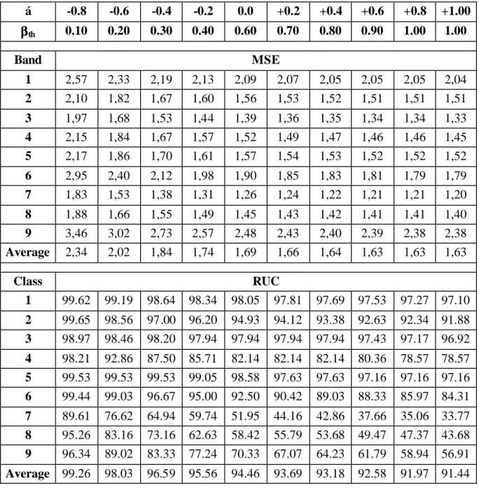
with step 0.1. As can be inferred from the tables and charts reported in this section, the proposed technique provides the expected results. In spite of the particular association criterion adopted in the encoding phase, which may cause a pixel to be assigned even to a very distant codevector, the visual quality of the encoded images was suitably preserved. This is confirmed also in the case of a dominant weight of the classification parameter in the cost function, which generates only limited MSE increases. The reason of this behavior is mainly imputable to the good configuration of the codebook, that is generated taking into account the cardinality and distribution of the classes.

Figs. 11-12 show the MSE and RUC values varying the codebook size and the classification factor for the two image sets. In particular it can be noticed that for low values of α, very low classification discrepancies are present (almost all image pixels are equally classified in the original and compressed image), while only a slight worsening in terms of MSE is introduced. From the observation of Figs. 11-12, the monotonic

behavior of the RUC in dependency of

á

(see § 3.1), with a maximum in

á

=-0.8 corresponding to the lower extreme of the

á

variability range is also evident.

Another important point is that the achieved classification improvement uniformly involves all the classes, whatever the number and distribution of their samples, as shown for “Feltwell” in Table II (for a codebook size M=512). This fact is even more evident for the set “Blue-bury” (reported in Table II), which is

characterized by a more unbalanced class distribution. In particular, the rows corresponding to less numerous classes (classes 7-9) show an increase in the rate of unchanged classification from 30-40% up to 90-95%, provided that the classification factor is set to a sufficiently low value. Such an improvement is reflected in minor increases in terms of average MSE (about 0.2 for “Feltwell” and 0.7 for “Blue-bury”).

As regards compression, it should be pointed out that baseline SCVQ, like SVQ, cannot achieve very high

CFs. This is due to the fact that the amount of compression can only be controlled by setting the codebook

size (see Eq. 1). Since it is not reasonable to reduce the size of the codebook below a given value (typically, 64 vectors), SCVQ does not allow to increase the compression arbitrarily. In particular, for "Feltwell" CF is in the range of 5.3÷8, while for “Blue-bury” the range is 8÷12, due to the larger number of spectral bands. Nevertheless, it is always possible to achieve very significant compression factors by exploiting the residual spatial redundancy, which is in general very high: in fact, differently from spatial VQ spectral VQ works on single pixels, thus preserving (or even increasing) the spatial correlation. Effective post-coding algorithms, capable of achieving sharp spatial redundancy reduction, can be introduced without modifying the proposed coding scheme, simply by working on the address stream generated by SCVQ. Although a specific analysis of these methods is beyond the scope of this paper, we here present some results achieved by a simple lossless post-coding approach. This method is based on a work by Poggi [15], and consists of a predictive coding of the VQ stream. In fact, the codebook is sorted in such a way as to have similar codevectors associated to near addresses, thus allowing to apply a DPCM-like technique to the sequence of VQ addresses. The algorithm was tested for different classification factors and codebook sizes, providing satisfactory results, as shown in Table III. As expected, only minor differences have been observed on

varying the

á

factor, while a higher performance was achieved on small codebooks, due to better prediction results. More complex post-coding approaches can also be adopted, if a higher performance is required, at the expense of heavier computation (see [16][17]).

In order to compare the performance of SCVQ to other competing approaches, specific tests have been implemented by considering two other classical compression methods widely used for R-S images: the standard JPEG and a three-dimensional transform coder (KLT-JPEG). In Fig. 13, the results are reported in terms of MSE (Fig. 13.a) and RUC percentage (Fig. 13.b) for the test set “Feltwell”, using a classification

for higher ranges of compression, while ensuring sufficiently low MSE values. The choice of the value

4

.

0

á

=

−

is very typical in our simulations, as it achieves a good compromise between improvement in classification performance and low MSE degradation. As a matter of fact, from the analysis of the charts in Figs. 11-12, it can be observed that the increase in MSE is very low for α > −0.3, while it is higher for

α < −0.5, due to the predominant weight of the classification factor in the cost function. On the contrary,

RUC values are characterized by a more uniform behavior. Therefore, a value of α in the range [-0.5,-0.3] ensures a significant improvement in the classification performance, without producing a notable damage from the visual standpoint.

Compared to the SVQ, the SCVQ algorithm presents an increase in computational complexity due to the introduction of a classifier in the encoder and to the use of a more complex cost function. Concerning classification let refer with N to the size of the feature vector and Z to the cardinality of the training set. Then, a standard k-NN classifier requires to compute the distance of each vector to each other in the training set, that requires ZN products + N(N-1) sums, and to order the resulting distances, that requires ZlogZ checks. Then the pixel is classified looking for the predominant class in the K vectors of the training that result to be the closest ones to the pixel to be classified. Accordingly, we can say that the computational complexity introduced with the k-NN classifier for each pixel is of the order of ZN products. Considered that the VQ encoding of the same pixel requires MN products, the increase in computation is not negligible, especially if a large training set is used compared to the codebook dimension M. Nevertheless, it is to be pointed out that SCVQ works irrespectively of the adopted classifier, thus allowing to choose a more computationally effective approach, such as the Bayesian or the Neural one.

Concerning the cost function, the two alternative schemes proposed in Fig. 8 show a different complexity. In the first case, if K is the number of classes, the additional computation required is summarized as follows: • NpelxM additional checks have to be performed in order to check whether each pair of image pixel and

codebook vector belong to the same class;

•

N

_pel

×

M

K

additional products of

d

_i,j with the scaling factor

2

1

+

α

(constant for every pixel) have

to be performed. This is in fact the number of times the image pixel and codevector belong to the same class.

In the second case, we need to perform an additional ordering of the

β

_i coefficients that introduces a computational complexity of

N

_pel

log

N

_pel.

This analysis shows that the modified cost function in the SCVQ algorithm introduces a negligible amount of processing respect to the classical SVQ, and only the use of the k-NN classifier can introduce some issues relevant to the computational complexity of the SCVQ algorithm.

A final remark regards the peculiarity of this technique of low visual impact on decompressed images, compared to classical block coding techniques. This property, which is derived from the basic SVQ technique, can be appreciated on observing Fig. 14, which compares a detail of band 4 of “Feltwell” compressed with SCVQ, SVQ, and the JPEG standard.

5. Conclusions

Based on the idea of Spectral Vector Quantization, a new approach to multispectral image compression for

remote sensing applications, called Spectral Classified Vector Quantization, has been presented. SCVQ combines a compression and a classification methodology into a single scheme, allowing the user to set the desired trade-off between classification accuracy and objective image quality (SNR). Two alternative

schemes are presented in which the interaction with the system simply consists of tuning a single parameter, thus rendering the use of the codec particularly intuitive even for unskilled users. Implementation suggestions are provided, mainly concerning the set up of encoder parameters and some tips are given for effective codebook design.

The technique was tested on several multispectral data sets, and experimental results showed that SCVQ can provide the expected performance. Further work is being conducted by the authors in order to test the efficiency of the presented technique for hyperspectral images. Preliminary experiments in this sense are giving encouraging results.

6. References

[1] J. A. Saghri, A. G. Tescher and J. T. Reagan, “Practical Transform Coding of Multispectral Imagery”,

[2] R. M. Gray, “Vector Quantization”, IEEE ASSP Magazine, vol. 1, pp. 4-29, April 1984

[3] M. Ryan and J. Arnold, “The lossless compression of AVIRIS images by vector quantization”, IEEE

Trans. On Geoscience and Remote Sensing, 35(3), pp. 546-550, May 1997

[4] S-E-Qian, A. Hollinger, D. Williams and D. Manak, “3D data compression of Hyperspectral imagery using vector quantization with NDVI-based multiple codebooks”, IGARSS 1998, Seattle, 6-10 July 1998

[5] G. F. McLean, “Vector Quantization for texture classification”, IEEE Trans. Systems, Man, and

Cybernetics, vol. 23, no. 3, pp. 637-649, May-Jun. 1993

[6] Q. Xie, C. A. Laszlo and R. K. Ward, “Vector quantization technique for nonparametric classifier design”, IEEE Trans. Pattern Analysis and Machine Intelligence, vol. 15, no. 12, pp. 1326-1330, Dec. 1993

[7] K. Popat and R. W. Picard, “Novel cluster based probability model for texture synthesis, classification and compression”, Proc. SPIE Visula Comm. And Image Processing, Boston, Nov. 1993

[8] K. Popat and R. W. Picard, “ Cluster based probability model applied to image restoration and compression”, Proc. ICASSP, Adelaide, Australia, 1994

[9] T. Kohonen, “Self-organization and Associative Memory”, Berlin: Springer-Verlag, 3rd ed., 1989 [10] T. Kohonen, G. Barna, and R. Chrisley, “Statistical pattern recognition with neural networks:

Benchmarking studies”, IEEE Int. Conf. Neural Networks, July 1988, pp. 61-68

[11] G. Mercier, M. C. Mouchot and G. Cazaguel, “Joint Classification and Compression of Hyperstpectral Images”, IGARSS’99, Hamburg, 28 June – 2 July 1999

[12] R.O. Duda & P.E. Hart, Pattern Classification and Scene Analysis, Wiley, New York, 1973.

[13] K. L. Oehler, R. M. Gray, “Combining Image Compression and Classification Using Vector Quantization”, IEEE Trans. On Pattern Analysis and Machine Intelligence, vol. 17, no. 5, pp. 461-473, May 1995,

[14] Y. Linde, A. Buzo, R. M. Gray, “An Algorithm for Vector Quantizer Design”, IEEE Transactions on

[15] G. Poggi, “Address-predictive vector quantization of images by topology-preserving codebook ordering”, European Transactions on Telecommunications and Related Technologies, vol. 4, pp. 423-434, July/August 1993

[16] N.M. Nasrabadi and Y. Feng, “Image compression using address-quantization”, IEEE Transactions on

Communication, vol. COM-38, pp. 2166-2173, December 1990

[17] F.G.B. De Natale, S. Fioravanti, and D.D. Giusto, “DCRVQ: a new strategy for efficient entropy coding of vector-quantized images”, IEEE Transactions on Communication, vol. COM-44, no. 6, pp. 696-706, Jan. 1996

List of Captions

Table I: MSE and RUC versus classification factor for “Feltwell” (M=512, CF=5.33) Table II: MSE and RUC versus classification factor for “Blue-bury” (M=512, CF=8.0)

Table III: compression ratio before and after applying the lossless spatial coding of [15] on varying the codebook dimension for “Feltwell” and “Blue-bury”

Figure 1: (a) Spectral VQ block diagram; (b) Codebook generation with LBG algorithm

Figure 2: Feltwell dataset (250x350 pels, 6 spectral bands at 8bpp), a detail of band 4 and its compressed versions (compression ratio 1:8) (a) Original, (b) SVQ, (c) JPEG

Figure 3: Blue-bury: compression impact on class average spectral signatures in the case M=64 Figure 4: Feltwell, performance comparison among SVQ, JPEG, and KLT-JPEG for increasing compression rates: (a) MSE , (b) RUC

Figure 5: Blue-bury, performance comparison among SVQ, JPEG, and KLT-JPEG for increasing compression rates: (a) MSE , (b) RUC

Figure 6: Assignment criterion: practical example in a 2D feature space

Figure 7: Graphic representation of the SCVQ method: (a) Euclidean distances of

v

r

_m and

v

r

_n from

x

r

_i (b) parametric distances defined in Eq. 5 of

v

r

_m and

v

r

_n from

x

r

_iin the case of α = 0.2, (c) α = -0.4, and (d) for α = −0.2 for which the two vectors have the same corrected distance from

x

i

r

Figure 8: Flowchart of the SCVQ coding algorithm: (a) coding driven by the α parameter (b) coding driven by the desired RUC parameter

Figure 9: Codebook initialization: definition of codevectors distribution by a polynomial function Figure 10: Codebook generation: MSE versus LBG iterations for (a) M=128, (b) M=256

Figure 11: MSE and RUC versus classification factor for “Feltwell” Figure 12: MSE and RUC versus classification factor for “Blue-bury”

Figure 13: Comparison among SCVQ (

á

=

−

0

.

4

), JPEG and KLT-JPEG in terms of (a) MSE and (b) RUC versus CF

Figure 14: Feltwell, 250x350 pels, 6 spectral bands at 8bpp: (a) a detail, (b) JPEG compressed (CF=9.5), (c) SVQ compressed (CF=9,07), (d) SCVQ compressed (CF=9.02,

á

=

−

0

.

6

)

Tables and figures

Table I

á

-0.8

-0.6

-0.4

-0.2

0.0

+0.2

+0.4

+0.6

+0.8

+1.00

ββ

th

0.10

0.20

0.30

0.40

0.60

0.70

0.80

0.90

1.00

1.00

Band

MSE

1

1,535 1,517 1,496 1,467 1,446 1,423 1,406 1,387 1,382 1,369

2

1,043 1,030 1,010 0,992 0,977 0,962 0,953 0,944 0,941 0,932

3

1,593 1,564 1,507 1,459 1,418 1,383 1,350 1,328 1,318 1,297

4

2,650 2,572 2,511 2,468 2,420 2,392 2,356 2,342 2,321 2,334

5

2,301 2,270 2,238 2,223 2,201 2,186 2,155 2,134 2,116 2,118

6

2,579 2,538 2,468 2,418 2,379 2,353 2,343 2,332 2,336 2,343

Average 1,950 1,915 1,872 1,838 1,807 1,783 1,760 1,745 1,736 1,732

Class

RUC

1

99,66 99,04 98,55 98,22 97,54 96,87 96,09 95,13 94,31 93,54

2

100,00 99,47 98,70 97,98 97,35 96,29 95,38 94,27 92,63 91,19

3

100,00 99,89 99,46 99,35 98,81 97,95 97,20 95,79 95,04 93,20

4

99,83 99,52 98,49 97,02 95,64 94,51 92,31 90,36 88,16 85,74

5

99,85 98,90 98,09 96,69 95,73 94,55 92,78 91,53 90,35 89,03 Average 99,85 99,34 98,59 97,73 96,85 95,86 94,53 93,18 91,75 90,18

Table II

á

-0.8

-0.6

-0.4

-0.2

0.0

+0.2

+0.4

+0.6

+0.8

+1.00

ββ

th

0.10

0.20

0.30

0.40

0.60

0.70

0.80

0.90

1.00

1.00

Band

MSE

1

2,57

2,33

2,19

2,13

2,09

2,07

2,05

2,05

2,05

2,04

2

2,10

1,82

1,67

1,60

1,56

1,53

1,52

1,51

1,51

1,51

3

1,97

1,68

1,53

1,44

1,39

1,36

1,35

1,34

1,34

1,33

4

2,15

1,84

1,67

1,57

1,52

1,49

1,47

1,46

1,46

1,45

5

2,17

1,86

1,70

1,61

1,57

1,54

1,53

1,52

1,52

1,52

6

2,95

2,40

2,12

1,98

1,90

1,85

1,83

1,81

1,79

1,79

7

1,83

1,53

1,38

1,31

1,26

1,24

1,22

1,21

1,21

1,20

8

1,88

1,66

1,55

1,49

1,45

1,43

1,42

1,41

1,41

1,40

9

3,46

3,02

2,73

2,57

2,48

2,43

2,40

2,39

2,38

2,38

Average

2,34

2,02

1,84

1,74

1,69

1,66

1,64

1,63

1,63

1,63

Class

RUC

1

99.62 99.19 98.64 98.34 98.05 97.81 97.69 97.53 97.27 97.10

2

99.65 98.56 97.00 96.20 94.93 94.12 93.38 92.63 92.34 91.88

3

98.97 98.46 98.20 97.94 97.94 97.94 97.94 97.43 97.17 96.92

4

98.21 92.86 87.50 85.71 82.14 82.14 82.14 80.36 78.57 78.57

5

99.53 99.53 99.53 99.05 98.58 97.63 97.63 97.16 97.16 97.16

6

99.44 99.03 96.67 95.00 92.50 90.42 89.03 88.33 85.97 84.31

7

89.61 76.62 64.94 59.74 51.95 44.16 42.86 37.66 35.06 33.77

8

95.26 83.16 73.16 62.63 58.42 55.79 53.68 49.47 47.37 43.68

9

96.34 89.02 83.33 77.24 70.33 67.07 64.23 61.79 58.94 56.91

Average 99.26 98.03 96.59 95.56 94.46 93.69 93.18 92.58 91.97 91.44

Table III Codebook size Technique 512 256 128 64 SCVQ 5.3 6 6.9 8 "Feltwell"

_{SCVQ + spatial}

coding

9.02 9.97 12.3 16 "Blue -bury"

SCVQ

8 9 10.3 12

SCVQ + spatial

coding

15.6 17 21.1 29

(a)

yes

no

(b)

Figure 1

(a)

(b)

(c)

Figure 2

Class 1 38 58 78 98 0 1 2 3 4 5 6 7 8 9 Orig VQ64 Class 2 34 44 54 64 74 84 0 1 2 3 4 5 6 7 8 9 Orig VQ64 Class 3 35 55 75 95 115 0 1 2 3 4 5 6 7 8 9 Orig VQ64 Class 4 40 50 60 70 0 1 2 3 4 5 6 7 8 9 Orig VQ64 Class 5 38 58 78 98 118 0 1 2 3 4 5 6 7 8 9 Orig VQ64 Class 6 44 54 64 74 84 0 1 2 3 4 5 6 7 8 9 Orig VQ64 Class 7 50 55 60 65 70 75 0 1 2 3 4 5 6 7 8 9 Orig VQ64 Class 8 40 50 60 70 0 1 2 3 4 5 6 7 8 9 Orig VQ64 Class 9 48 58 68 78 0 1 2 3 4 5 6 7 8 9 Orig VQ64

Figure 3

0.5 1 1.5 2 2.5 3 3.5 5 5.5 6 6.5 7 7.5 8 8.5 9 9.5 10 SVQ JPEG KLT-JPEG CF MSE 82 84 86 88 90 92 94 5 5.5 6 6.5 7 7.5 8 8.5 9 9.5 10 CF RUC SVQ JPEG KLT-JPEG

(a)

(b)

Figure 4

0.5 1 1.5 2 2.5 3 3.5 4 4.5 6 7 8 9 10 11 12 13 MSE CF SVQ JPEG KLT-JPEG

86 87 88 89 90 91 92 6 7 8 9 10 11 12 13 14 15 CF RUC SVQ JPEG KLT-JPEG

(a)

(b)

Figure 5

Figure 6

(a)

(b)

(c)

(d)

Figure 7

Figure 8 (a)

CLASSIFIER ENCODER i p ∀ find       ₌ + 2 1 min _{ij ij} ij j c d D ENTROPY CODER

α

α

Input Dataset Coded Image Codebook

CLASSIFIER i p ∀

(

d v anyclass

)

find im m m , ∈ min

(

in n i

)

n d v same class of p findmin , ∈ n i m i i d d n m store , ,β = _, / _, ENTROPY CODER Desired RUC Input Dataset Coded Image Codebook

order the array βi àβˆ i

select β*=βˆi, i=Npel⋅RUC/100

' ' ' ' * n address emit else m address emit if p_i β_i>β ∀

Figure 8 (b)

max , c

N

N

c

Figure 9

M=128 2,2 2,4 2,6 2,8 3 3,2 3,4 1 2 3 4 5 6 7 8 9 10 11 12 13 14 15 Iteration MSE

random proportional cubic root cubic

M=256 1,5 1,8 2,1 2,4 2,7 3 1 2 3 4 5 6 7 8 9 10 11 12 13 14 15 Iteration MSE

random proportional cubic root cubic

(a)

(b)

Figure 10

Feltwell 0 1 2 3 4 5 -0,8 -0,6 -0,4 -0,2 0 0,2 0,4 0,6 0,8 1 α α MSE 64 128 256 512

Feltwell 84 86 88 90 92 94 96 98 100 102 -0,8 -0,6 -0,4 -0,2 0 0,2 0,4 0,6 0,8 1 α α RUC 64 128 256 512

Figure 11

Blue-bury 0 1 2 3 4 5 6 7 -0,8 -0,6 -0,4 -0,2 0 0,2 0,4 0,6 0,8 1 α α MSE 64 128 256 512

Blue-bury 87 89 91 93 95 97 99 -0,8 -0,6 -0,4 -0,2 0 0,2 0,4 0,6 0,8 1 α α RUC 64 128 256 512

Figure 12

Feltwell 0,0 0,5 1,0 1,5 2,0 2,5 3,0 3,5 4,0 4,5 5,0 9 , 0 0 10,00 12,00 16,00 C F M S E S C V Q J P E G K L T - J P E G

Feltwell 91 93 95 97 99 9,00 10,00 12,00 16,00 CF RUC SCVQ JPEG KLT-JPEG

Figure 13

(a)

(b)

(c)

(d)

Figure 14