Technical Report CoSBi 07/2006
Modelling Cellular Processes using
Membrane Systems with Peripheral and
Integral Proteins
Matteo CavaliereThe Microsoft Research – University of Trento Centre for Computational and Systems Biology
Sean Sedwards
The Microsoft Research – University of Trento Centre for Computational and Systems Biology
This is a preliminary version of a paper that will appear in
Proceedings of the International Conference on Computational Methods in Systems Biology, CMSB06, Lecture Notes in Bioinformatics, 4210:108–126, 2006.
Abstract
Membrane systems were introduced as models of computation inspired by the structure and functioning of biological cells. Recently, membrane systems have also been shown to be suitable to model cellular processes. We introduce a new model called Membrane Systems with Peripheral and Integral Proteins. The model has compartments enclosed by membranes, floating objects, objects associated to the internal and external surfaces of the membranes and also objects integral to the membranes. The floating objects can be processed within the compartments and can interact with the objects associated to the membranes. The model can be used to represent cellular processes that involve compartments, surface and integral membrane proteins, transport and processing of chemical substances. As examples we model a circadian clock and the G-protein cycle in yeast saccharomyces cerevisiae and present a quantitative analysis using an implemented simulator.
1
Introduction
Membrane systems are models of computation inspired by the structure and the function of biological cells. The model was introduced in 1998 by Gh. P˘aun and since then many results have been obtained, mostly concerning computational power. A short introduc-tory guide to the field can be found in [12], while an updated bibliography is available via the web-page [18]. Recently (see, e.g., [10]), membrane systems have been successfully applied to systems biology and several models have been proposed for simulating biolog-ical processes (e.g., see the monograph dedicated to membrane computing applications [5]).
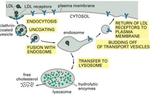
By the original definition, membrane systems are composed of an hierarchical nest-ing of membranes that enclose regions (the cellular structure), in which free-floatnest-ing objects (molecules) exist. Each region can have associated rules, called evolution rules, for evolving the free-floating objects and modelling the biochemical reactions present in cell regions. Rules also exist for moving objects across membranes, called symport and antiport rules, modelling cellular transport. Recently, inspired by brane calculus [3], a model of a membrane system, having free-floating objects and objects attached to the membranes, was introduced in [2]. The attached objects model the proteins that are embedded in lipid bilayer cell membranes. In [2], however, objects are associated to an indivisible membrane which has no concept of inner or outer surface, while in [4] ob-jects (peripheral proteins) are attached to either side of a membrane. In reality, many biological processes are driven and controlled by the presence of specific proteins on the appropriate side of and integral to the membrane: there is a constant interaction between floating chemicals and embedded proteins and between peripheral and integral proteins (see, e.g., [1]). Receptor-mediated processes, such as endocytosis (illustrated in Figure 1) and signalling, are crucial to cell function and by definition are critically dependent on the presence of peripheral and integral membrane proteins.
One model of the cell is that of compartments and sub-compartments in constant communication, with molecules being passed from donor compartments to target com-partments by interaction with membrane proteins. Once transported to the correct
Figure 1: Endocytosis of LDL (Essential Cell Biology, 2/e, c 2004 Garland Science)
compartment, the substances are then processed by means of local biochemical reactions. Motivated by these ideas we extend the model presented in [4], introducing a model having peripheral as well as integral proteins.
In each region of the system there are floating objects (the floating chemicals) and, in addition, objects can be associated to each side of a membrane or integral to the membrane (the peripheral and integral membrane proteins). Moreover, the system can perform the following operations: (i) the floating objects can be processed/changed inside the regions of the system (emulating biochemical rules) and (ii) the floating and attached objects can be processed/changed when they interact (modelling the interactions of the floating molecules with membrane proteins).
The proposed model can be used to represent cellular processes that involve floating molecules, surface and integral membrane proteins, transport of molecules across mem-branes and processing of molecules inside the compartments. As examples, we model a circadian clock and the G-protein cycle in saccharomyces cerevisiae, where the possibil-ity to use, in an explicit way, compartments, membrane proteins and transport rules is very useful. A quantitative analysis of the models is also presented, performed using an extended version of the simulator presented in [4] (downladable at [19]). The simulator employs a stochastic algorithm and uses intuitive syntax based on chemical equations (described in appendix B).
2
Formal Language Preliminaries
Membrane systems are based on formal language theory and multiset rewriting. We now briefly recall the basic theoretical notions used in this paper. For more details the reader can consult standard books, such as [8], [15], [6] and handbook [14].
Given the set A we denote by |A| its cardinality and by ∅ the empty set. We denote by N and by R the set of natural and real numbers, respectively.
As usual, an alphabet V is a finite set of symbols. By V∗ we denote the set of all strings over V . By V+ we denote the set of all strings over V excluding the empty
string. The empty string is denoted by λ. The length of a string v is denoted by |v|. The concatenation of two strings u, v ∈ V∗ is written uv.
A multiset is a set where each element may have a multiplicity. Formally, a multiset over a set V is a map M : V → N, where M (a) denotes the multiplicity of the symbol a ∈ V in the multiset M .
For multisets M and M0 over V , we say that M is included in M0 if M (a) ≤ M0(a) for all a ∈ V . Every multiset includes the empty multiset, defined as M where M (a) = 0 for all a ∈ V .
The sum of multisets M and M0 over V is written as the multiset (M + M0), defined by (M + M0)(a) = M (a) + M0(a) for all a ∈ V . The difference between M and M0 is written as (M − M0) and defined by (M − M0)(a) = max{0, M (a) − M0(a)} for all a ∈ V . We also say that (M + M0) is obtained by adding M to M0 (or viceversa) while (M − M0) is obtained by removing M0 from M . For example, given the multisets M = {a, b, b, b} and M0 = {b, b}, we can say that M0 is included in M , that (M + M0) = {a, b, b, b, b, b} and that (M − M0) = {a, b}.
If the set V is finite, e.g. V = {a1, . . . , an}, then the multiset M can be explicitly
described as {(a1, M (a1)), (a2, M (a2)), . . . , (an, M (an))}. The support of a multiset M is
defined as the set supp(M ) = {a ∈ V | M (a) > 0}. A multiset is empty (hence finite) when its support is empty (also finite).
A compact notation can be used for finite multisets: if M = {(a1, M (a1)), (a2, M (a2)),
. . . , (an, M (an))} is a multiset of finite support, then the string w = a M (a1) 1 a M (a2) 2 . . . a M (an) n
(and all its permutations) precisely identify the symbols in M and their multiplicities. Hence, given a string w ∈ V∗, we can say that it identifies a finite multiset over V , writ-ten as M (w), where M (w) = {a ∈ V | (a, |w|a)}. For instance, the string bab represents
the multiset M (w) = {(a, 1), (b, 2)}, that is the multiset {a, b, b}. The empty multiset is represented by the empty string λ.
3
Operations with Peripheral and Integral Proteins
Let V denote a finite alphabet of objects and Lab a finite set of labels.
As is usual in the membrane systems field, a membrane is represented by a pair of square brackets, [ ]. A membrane structure is an hierarchical nesting of membranes enclosed by a main membrane called the root membrane. To each membrane is associated a label that is written as a superscript of the membrane, e.g. [ ]1. If a membrane has the
label i we call it membrane i.
A membrane structure is essentially that of a tree, where the nodes are the membranes and the arcs represent the containment relation. In this paper we avoid a formal mapping in the interest of the intuitiveness of the description, however, being a tree, a membrane structure can be represented by a string of matching square brackets, e.g., [ [ [ ]2 ]1 [ ]3 ]0.
To each membrane there are associated three multisets, u, v and x over V , denoted by [ ]u|v|x. We say that the membrane is marked by u, v and x; x is called the external
marking, u the internal marking and v the integral marking of the membrane. In general, we refer to them as markings of the membrane.
The internal, external and integral markings of a membrane model the proteins at-tached to the internal surface, atat-tached to the external surface and integral to the
mem-brane, respectively.
In a membrane structure, the region between membrane i and any enclosed mem-branes is called region i. To each region is associated a multiset of objects w called the free objects of the region. The free objects are written between the brackets enclosing the regions, e.g., [ aa [ bb ]1 ]0.
The free objects of a membrane model the floating chemicals within the regions of a cell.
We denote by int(i), ext(i) and itgl(i) the internal, external and integral markings of membrane i, respectively. By f ree(i) we denote the free objects of region i. For any membrane i, distinct from a root membrane, we denote by out(i) the label of the membrane enclosing membrane i.
For example, the string
[ ab [ cc ]2a| | [ abb ]1bba|ab|c ]0
represents a membrane structure, where to each membrane are associated markings and to each region are associated free objects. Membrane 1 is internally marked by bba (i.e., int(1) = bba), has integral marking ab (i.e., itgl(1) = ab) and is externally marked by c (i.e., ext(1) = c). To region 1 are associated the free objects abb (i.e., f ree(1) = abb). To region 0 are associated the free objects ab. Finally, out(1) = out(2) = 0. Membrane 0 is the root membrane. The string can also be depicted diagrammatically, as in Figure 2.
Figure 2: Graphical representation of [ ab [ cc ]2
a| | [ abb ] 1 bba|ab|c ]
0
When a marking is omitted it is intended that the membrane is marked by the empty string λ, i.e., the empty multiset. For instance, in [ ab ]u|v| the external marking is
missing, while in the case of [ ab ]|v|x the internal marking is missing.
3.1
Operations
We introduce rules that describe bidirectional interactions of floating objects with the membrane markings which we call membrane rules. These rules are motivated by the behaviour of cell membrane proteins (e.g., see [1]) and therefore permit a level of abstrac-tion based on the behaviour of real molecules. We denote the rules as attachin, attachout,
attachin : [ α ]iu|v| → [ ] i
u0|v0|, α ∈ V+, u, v, u0, v0 ∈ V∗, i ∈ Lab
attachout : [ ]i|v|xα → [ ]i|v0|x0 , α ∈ V+, v, x, v0, x0 ∈ V∗, i ∈ Lab
de − attachin : [ ]iu|v| → [ α ]iu0|v0|, α, u0, v0, u, v ∈ V∗, |uv| > 0, i ∈ Lab
de − attachout : [ ]i|v|x → [ ]i|v0|x0α, α, v0, x0, v, x ∈ V∗, |vx| > 0, i ∈ Lab
The semantics of these rules is as follows.
The attachin rule is applicable to membrane i if f ree(i) includes α, int(i) includes
u and itgl(i) includes v. When the rule is applied to membrane i, α is removed from f ree(i), u is removed from int(i), v is removed from itgl(i), u0 is added to int(i) and v0 is added to itgl(i). The objects not involved in the application of the rule are left unchanged in their original positions.
The attachout rule is applicable to membrane i if f ree(out(i)) includes α, itgl(i)
includes v, ext(i) includes x. When the rule is applied to membrane i, α is removed from f ree(out(i)), v is removed from itgl(i), x is removed from ext(i), v0 is added to itgl(i) and x0 is added to ext(i). The objects not involved in the application of the rule are left unchanged in their original positions.
The de − attachin rule is applicable to membrane i if int(i) includes u and itgl(i)
includes v. When the rule is applied to membrane i, u is removed from int(i), v is removed from itgl(i), u0 is added to int(i), v0 is added to itgl(i) and α is added to f ree(i). The objects not involved in the application of the rule are left unchanged in their original positions.
The de − attachout rule is applicable to membrane i if itgl(i) includes v and ext(i)
includes x. When the rule is applied to membrane i, v is removed from itgl(i), x is removed from ext(i), v0 is added to itgl(i), x0 is added to ext(i) and α is added to f ree(out(i)). The objects not involved in the application of the rule are left unchanged in their original positions.
We denote by Ratt
V,Lab the set of all possible attach and de − attach rules over the
alphabet V and set of labels Lab. Instances of attachin, attachout, de − attachin and
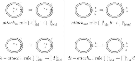
de − attachout rules are depicted in Figure 3.
We next introduce evolution rules that rewrite the free objects contained in a region conditional on the markings of the enclosing membrane. These rules can be considered to model the biochemical reactions that take place within the cytoplasm of a cell. We define an evolution rule:
evol : [ α → β ]iu|v|
where u, v, β ∈ V∗, α ∈ V+, and i ∈ Lab.
The semantics of the rule is as follows. The rule is applicable to region i if f ree(i) includes α, int(i) includes u and itgl(i) includes v. When the rule is applied to region
attachin rule [ b ]ib|c|→ [ ]idb|c| attachout rule [ ]i|c|a b → [ ]i|c|ad
de − attachin rule [ ]ibb|c| → [ d ]ib|c| de − attachout rule [ ]i|c|a → [ ]i| |a d
Figure 3: Examples of attachin, attachout, de − attachin and de − attachout rules, showing
how free and attached objects may be rewritten. E.g., in the attachin rule one of the two
free instances of b is rewritten to d and added to the membrane’s internal marking.
Figure 4: evol rule [ a → b ]ib|c|. Free objects can be rewritten inside the region and the rewriting can depend on the integral and internal markings of the enclosing membrane.
i, α is removed from f ree(i) and β is added to f ree(i). The membrane markings and the objects not involved in the application of the rule are left unchanged in their original positions.
We denote by Rev
V,Lab the set of all evolution rules over the alphabet V and set of
labels Lab. An instance of an evolution rule is represented in Figure 4.
In general, when a rule has label i we say that a rule is associated to membrane i (in the case of attach and de − attach rules) or is associated to region i (in the case of evol rules). For instance, in Figure 3 the attachin is associated to membrane i.
The objects of α, u and v for attachin/evol rules, of α, v and x for attachout rules, of
u and v for de − attachin rules and of v and x for de − attachout rules are the reactants
of the corresponding rules. E.g., in the attach rule [ b ]a|c| → [ ]d|c|, the reactants are a,
b and c.
We note that a single application of an evol rule may be simulated by an application of an attachin rule followed by an application of an de − attachin rule. This may be biologically
4
Membrane Systems with Peripheral and Integral
Proteins
In this section we define membrane systems having membranes marked with peripheral proteins, integral proteins, free objects and using the operations introduced in Section 3.
Definition 4.1 A membrane system with peripheral and integral proteins and n mem-branes (in short, a Ppi system), is a construct
P = (VP, µP, (u0, v0, x0)P, . . . , (un−1, vn−1, xn−1)P, w0,P, . . . , wn−1,P, RP, tin,P, tf in,P, rateP)
• VP is a finite, non-empty alphabet of objects.
• µP is a membrane structure with n ≥ 1 membranes injectively labelled by labels in LabP = {0, 1, · · · , n − 1}, where 0 is the label of the root membrane.
• (u0, v0, x0)P = (λ, λ, λ), (u1, v1, x1)P, · · · , (un−1, vn−1, xn−1)P ∈ V
∗ × V∗ × V∗ are
called initial markings of the membranes.
• w0,P, w1,P, · · · , wn−1,P ∈ V∗ are called initial free objects of the regions.
• RP ⊆ RattV,Lab
P−{0}∪R
ev
V,LabP is a finite set of evolution rules, attach/de-attach rules. 1
• tin,P, tf in,P ∈ R are called the initial time and the final time, respectively. • rateP : RP 7−→ R is the rate mapping. It associates to each rule a rate.
Let Π be an arbitrary Ppi system. An instantaneous description I of Π consists of
the membrane structure µΠ with markings associated to the membranes and free objects associated to the regions. We denote by I(Π) the set of all instantaneous descriptions of Π. We say in short membrane (region) i of I to denote the membrane (region, respectively) i present in I.
Let I be an arbitrary instantaneous description from I(Π) and r an arbitrary rule from RΠ. Suppose that r is associated to membrane i ∈ LabΠ if r ∈ RattV,LabΠ−{0} (or to
region i ∈ LabΠ if r ∈ RevV,LabΠ).
Then, if r is applicable to membrane i (or to region i, accordingly) of I, in short we say that r is applicable to I. We denote by r(I) ∈ I(Π) the instantaneous description of Π obtained when the rule r is applied to membrane i (or to region i, accordingly) of I (in short, we say r is applied to I).
The initial instantaneous description of Π, Iin,Π ∈ I(Π), consists of the membrane
structure µΠ with membrane i marked by (ui, vi, xi)Π for all i ∈ LabΠ− {0} and free
objects wi,Π associated to region i for all i ∈ LabΠ.
1The root membrane may contain objects and evolution rules but not attach or de − attach rules,
since it has no enclosing region. It may therefore be viewed as an extended version of a membrane systems environment (as defined in [12]), with objects and evol rules. Alternatively, it can be seen as a membrane systems skin membrane, where the environment contains nothing and is not accessible.
A configuration of Π is a pair (I, t) where I ∈ I(Π) and t ∈ R; t is called the time of the configuration. We denote by C(Π) the set of all configurations of Π. The initial configuration of Π is Cin,Π = (Iin,Π, tin,Π).
Suppose that RΠ = {rule1, rule2, . . . , rulem} and let S be an arbitrary sequence of
configurations hC0, C1, · · · , Cj, Cj+1, · · · , Chi, where Cj = (Ij, tj) ∈ C(Π) for 0 ≤ j ≤ h.
Let aj = m
P
i=1
pi
j, 0 ≤ j ≤ h, where pij is the product of rate(rulei) and the mass action
combinatorial factor for rulei and I
j (see Appendix A).
The sequence S is an evolution of Π if • for j = 0, Cj = Cin,Π
• for 0 ≤ j ≤ h − 1, aj > 0, Cj+1= (rj(Ij), tj + dtj) with rj, dtj as in [7]:
– rj = rulek, k ∈ {1, · · · , m} and k satisfies k−1 P i=1 pi j < ran 0 j · aj ≤ k P i=1 pi j – dtj = (−1/aj)ln(ran 00 j)
where ran0j, ran00j are two random variables over the sample space (0, 1], uniformly distributed.
• for j = h, aj = 0 or tj ≥ tf in,Π.
In other words, an evolution of Π is a sequence of configurations, starting from the initial configuration of Π, where, given the current configuration Cj = (Ij, tj), the next one, Cj+1 =
(Ij+1, tj+1), is obtained by applying the rule rj to the current instantaneous description Ij and
adding dtj to the current time tj. The rule rj is applied as described in Section 3. Rule rj and
dtj are obtained using the Gillespie algorithm [7] over the current instantaneous description Ij.
The evolution halts when all rules have zero probability of being applied (aj = 0) or when the
current time is greater or equal to the specified final time.
5
Modelling and Simulation of Cellular Processes
Having established a theoretical basis, we now wish to demonstrate the quantitative behaviour of the presented model. To this end we have extended the simulator presented in [4] to produce evolutions of an arbitrary Ppi system. In Sections 5.2 and 5.3 we
demonstrate the model and the simulator using two examples from the literature.
5.1
The Stochastic Algorithm
We use a discrete stochastic algorithm based on Gillespie’s which can more accurately represent the dynamical behaviour of small quantities of reactants, in comparison, say, to a deterministic approach based on ordinary differential equations [11]. Moreover, Gillespie has shown that the algorithm is fully equivalent to the chemical master equation.
The Gillespie algorithm is specifically designed to model the interaction of chemical species and imposes a restriction of a maximum of three reacting molecules. This is on the basis that the likelihood of more than three molecules colliding is vanishingly small. Hence the simulator is similarly restricted. Note that in the evolution of a Ppisystem, the
stochastic algorithm does not distinguish between floating objects and objects attached or integral to the membrane. That is, the algorithm is applied to the objects irrespective of where they are in the compartment on the assumption that the interaction between floating and attached molecules can be considered the same as between floating molecules. Our application of the Gillespie algorithm to membranes is further described in Appendix A.
5.2
Modelling a Noise-Resistant Circadian Clock
Many organisms use circadian clocks to synchronise their metabolisms to a daily rhythm, however the precise mechanisms of implementation vary from species to species. One common requirement is the need to maintain a measure of stability of timing in the face of perturbations of the system: the clock must continue to tick and keep good time. A general model which captures the essence of such stability, based on common elements of several real biological clocks, is presented in [16]. We choose this as an interesting, non-trivial example to model and simulate with a Ppisystem using evolution rules alone.
Moreover, we choose this example because it has been modelled in other formalisms, such as in stochastic Π calculus (see, e.g., [17], [13]).
The model is described diagrammatically in Figure 5. The system consists of two dif-ferent genes (gA and gR) which produce two difdif-ferent proteins (pA and pR, respectively) via two different mRNA species (mA and mR, respectively). Protein pA up-regulates the transcription of its own gene and also the transcription of the gene that produces pR. The proteins are removed from the system by simple degradation to nothing (dashed lines) and by the formation of a complex AR. In this latter way the production of pR reduces the concentration of pA and has the consequence of down-regulating pR’s own production. Thus, in turn, pA is able to increase, increasing the production of pR and causing the cycle to repeat. Key elements of the stable dynamics are the rapid production of pA, by virtue of positive feedback, and the relative rate of growth of the complexation reaction.
A description of the Ppi system used to model the circadian clock is given in Figure 6,
together with the corresponding simulator script for comparison. The alphabet, Vclock, is
specified to contain all the reacting species. This corresponds to theobjectstatement of
the simulator script. The sixteen chemical reactions of Figure 5 are simply transcribed into corresponding rules mapped to reaction rates. In the simulator script they are grouped under one identifier, clock. The membrane structure, µclock, comprises just the
root membrane. The root region initially contains one copy each of the two genes as free objects. These facts are reflected in the systemstatement of the simulator script, which also associates to the contents the set of rules clock.
The results of running the script are shown in Figure 5: the two proteins exhibit anti-phase periodicity of approximately 24 hours, as expected.
Figure 5: Reaction scheme and simulation results of noise-resistant circadian clock of [16]
The simulator has the capability to add or subtract reactants from the simulation in runtime. We use this facility to discover the effect of switching off gR in the circadian clock by making the following addition to the systemstatement:
-1 gR @50000, -1 g R @50000
These instructions request a subtraction from the system at time step 50000 of one gR and one g R. Note that to switch off the gene it is necessary to remove both versions (i.e., with and without pA bound), since it is not possible to know in what state it will exist at a particular time step. Negative quantities are not allowed in the simulator, so only the existent specie will be deleted. In general, the number subtracted is the minimum of the existent quantity and the requested amount. The same syntax, without the negative sign, is used to add reactants.
The effect of switching off gR, shown in Figure 7, is to reduce the amount of pR to near zero and to thus allow pA to reach a maximum governed by its relative rates of production and decay. Note that a small amount of pR continues to exist long after its gene has been switched off. This is the result of a so-called hidden pathway from the AR complex, which decays at a much slower rate than pR (second graph of Figure 7). Although this model is a generalisation of biological circadian clocks and may not represent the behaviour of a specific example, the existence of an unexpected pathway exemplifies an important problem encountered when attempting to predict the behaviour of biological systems.
5.3
Modelling Saccharomyces Cerevisiae Mating Response
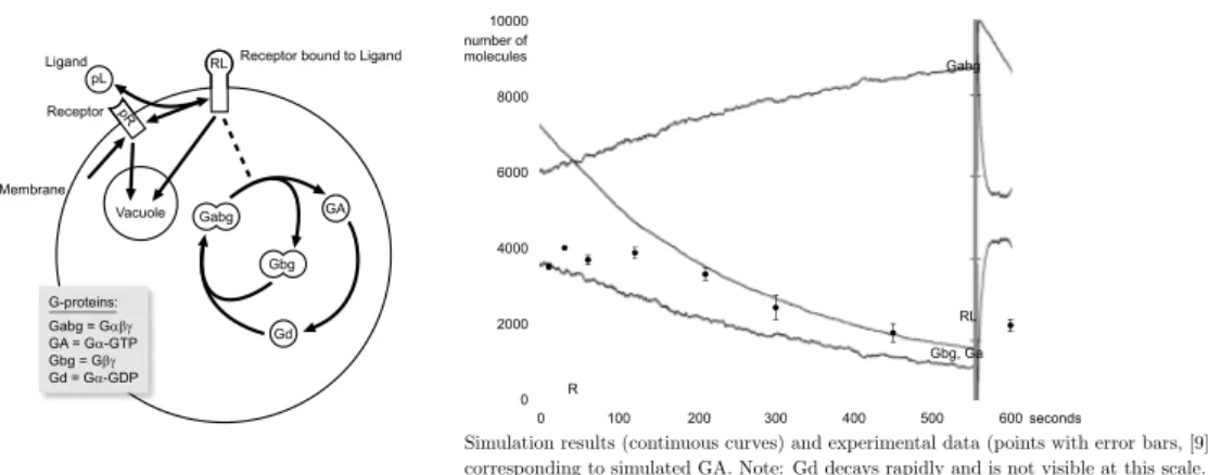
To demonstrate the ability of Ppi systems to represent compartments and membraneswe model and simulate the G-protein mating response in yeast saccharomyces cerevisiae, based on experimental rates provided by [9]. The G-protein transduction pathway in-volves membrane proteins and the transport of substances between regions and is a mechanism by which organisms detect and respond to environmental signals. It is exten-sively studied and many pharmaceutical agents are aimed at components of the G-protein cycle in humans. The diagram in Figure 8 shows the relationships between the various reactants and regions modelled and simulated.
Ppi system clock Simulator script
Vclock= {gA, g A, gR, g R, mA, mR, pA, pR, RA} object gA,g A,gR,g R,mA,mR,pA,pR,RA
rateclock= rule clock
{ { [ gA → gA mA ]0 | | 7→ 50 gA 50-> gA + mA [ pA gA → g A ]0 | | 7→ 1 pA+gA 1-> g A [ g A → g A mA ]0 | | 7→ 500 g A 500-> g A + mA [ gR → gR mR ]0 | | 7→ 0.01 gR 0.01-> gR + mR [ g R → g R mR ]0 | | 7→ 50 g R 50-> g R + mR [ mA → pA ]0 | | 7→ 50 mA 50-> pA [ mR → pR ]0 | | 7→ 5 mR 5-> pR [ pA pR → AR ]0 | | 7→ 2 pA+pR 2-> AR [ AR → pR ]0| | 7→ 1 AR 1-> pR [ pA → λ ]0| | 7→ 1 pA 1-> 0A [ pR → λ ]0 | | 7→ 1 pR 0.2-> 0R [ mA → λ ]0 | | 7→ 10 mA 10-> 0mA [ mR → λ ]0 | | 7→ 0.5 mR 0.5-> 0mR [ g R → pA gR ]0 | | 7→ 100 g R 100-> pA+gR [ pA gR → g R ]0 | | 7→ 1 pA+gR 1-> g R [ g A → pA gA ]0 | | 7→ 50 g A 50-> pA+gA } }
w0,clock= gA gR system 1 gA, 1 gR, clock
µclock= [ ]0
tin,clock= 0 evolve 0-150000
tf in,clock= 155 hours
plot pA, pR
Figure 6: Ppisystem model of circadian clock of [16] with corresponding simulator script.
Note the similarities between the definitions of Vclock andobjectand between the
defini-tions of the elements of rateclock and of rule clock.
(pL) which binds to a receptor pR, integral to the cell membrane. The receptor-ligand dimer then catalyses (dotted line in the diagram of Figure 8) the reaction that converts the inactive G-protein Gabg to the active GA. A competing sequence of reactions, which dominate in the absence of RL, converts GA to Gabg via Gd in combination with Gbg. The bound and unbound receptor (RL and pR, respectively) are degraded by transport into a vacuole via the cytoplasm. Figure 9 contains the Ppi system model and
corre-sponding simulator script. Note that while additional quantities of the receptor pR are created in runtime, no species is deleted from the system; the dynamics are created by transport alone.
Figure 8 shows the results of the stochastic simulation plotted with experimental re-sults from [16] equivalent to simulated GA. There is an apparent correspondence between the simulated and experimental data, in line with the deterministic simulation presented in the original paper. The stochastic noise evident in Figure 8 may explain why some measured points do not lie exactly on the deterministic curve, however further analysis of the original model is beyond the scope of this paper.
Figure 7: Simulated effect of switching off gA in circadian clock of [16]
Simulation results (continuous curves) and experimental data (points with error bars, [9]) corresponding to simulated GA. Note: Gd decays rapidly and is not visible at this scale.
Figure 8: Model and simulation results of saccharomyces cerevisiae mating response.
6
Prospects
We have introduced a model of membrane systems (called a Ppi system) with objects
integral to the membrane and objects attached to either side of the membrane. We have also introduced operations that can rewrite floating objects conditional on the existence of integral and attached objects and operations that facilitate the interaction of floating objects with integral and attached objects. With these we are able to model in detail many real biochemical processes occurring in the cytoplasm and in the cell membrane.
Evolutions of a Ppi system are obtained using an algorithm based on Gillespie [7] and
in the second part of the paper we have presented a simulator which can produce evolu-tions of an arbitrary Ppi system, using syntax based on chemical equations. To
demon-strate the utility of Ppi systems and of the simulator we have modelled and simulated
a circadian clock and the G-protein cycle mating response of saccharomyces cerevisiae. The latter makes extensive use of membrane operations.
Several different research directions are now proposed. The primary direction is the application of Ppi systems and of the simulator to real biological systems, with the aim
of prediction by in-silico experimentation. Such application is likely to lead to the need for new bio-inspired features and these constitute another direction of research. The features will be implemented in the model and simulator as necessary, however it is already envisaged that operations of fission and fusion will be required to permit the modification of a membrane structure in runtime.
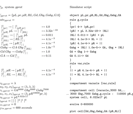
Ppi system gprot Simulator script
Vgprot= {pL, pr, pR, RL, Gd, Gbg, Gabg, GA} object pL,pr,pR,RL,Gd,Gbg,Gabg,GA rategprot= rule g cycle
{ { [ ]1 |pr|→ [ ]1|pR pr| 7→ 4.0 |pr| 4-> |pR,pr| [ ]1 |pR|pL → [ ]1|RL| 7→ 3.32e −18 |pR| + pL 3.32e-18-> |RL| [ ]1 |RL|→ [ ]1|pR|pL 7→ 0.011 |RL| 0.011-> |pR| + pL [ ]1|RL|→ [ RL ]1 | | 7→ 4.1e −3 |RL| 4.1e-3-> RL + || [ ]1|pR|→ [ pR ]1 | | 7→ 4.1e −4 |pR| 4.1e-4-> pR + || [ Gabg → GA Gbg ]1 |RL| 7→ 1.0e
−5 Gabg + |RL| 1.0e-5-> GA, Gbg + |RL|
[ Gd Gbg → Gabg ]1
| | 7→ 1.0 Gd + Gbg 1-> Gabg
[ GA → Gd ]1
| | 7→ 0.11 GA 0.11-> Gd
}
rule vac rule { [ ]2 | |pR → [ pR ]2| | 7→ 4.1e −4 || + pR 4.1e-4-> pR + || [ ]2| |RL → [ RL ]2| | 7→ 4.1e−3 || + RL 4.1e-3-> RL + || } }
w2,gprot= λ compartment vacuole [vac rule]
(u2, v2, x2)gprot= (λ, λ, λ)
w1,gprot= Gd3000Gbg3000Gabg7000 compartment cell [vacuole,3000 Gd,...
(u1, v1, x1)gprot= (λ, pR10000pr, λ) ... 3000 Gbg,7000 Gabg,g cycle : |10000 pR,pr|] w0,gprot= pL6.022e17 system cell, 6.022e17 pL
µgprot= [ [ [ ]2]1]0
tin,gprot= 0 evolve 0-600000 tf in,gprot= 600 seconds
plot cell[Gd,Gbg,Gabg,GA:|pR,RL|]
Figure 9: Ppi system model of G-protein cycle and corresponding simulator script.
A further direction of research is the investigation of the theoretical properties of the model. Reachability of configurations and of markings have already been proved to be decidable for the more restricted model presented in [4] and these proofs should be extended accordingly for the model presented here. Other work in this area might include the modification of the way a Ppi system evolves, for example, to allow other semantics
(such as that of maximal parallel [12]) or to use algorithms that more accurately model the behaviour of biological membranes. In this way we will be able to explore the limits of the model and perhaps discover a more useful level of abstraction.
References
[1] B. Alberts, A. Johnson, J. Lewis, M. Raff, K. Roberts, P. Walter, Molecular Biology of the Cell, 4th Ed., Garland Science, 2002, p. 593.
[2] R. Brijder, M. Cavaliere, A. Riscos-N´u˜nez, G. Rozenberg, D. Sburlan, Membrane Systems with Marked Membranes.Electronic Notes in Theoretical Computer Science. To appear.
[3] L. Cardelli, Brane Calculi. Interactions of Biological Membranes. Proceedings Computational Meth-ods in System Biology 2004 (V. Danos, V. Sch¨achter, eds.), Lecture Notes in Computer Science, 3082, Springer-Verlag, Berlin, 2005.
[4] M. Cavaliere, S. Sedwards, Membrane Systems with Peripheral Proteins: Transport and Evolution. Proceedings of MeCBIC06, Electronic Notes in Theoretical Computer Science, 171:2, pp. 37–53, 2007.
[5] G. Ciobanu, Gh. P˘aun, M.J. P´erez-Jim´enez, eds., Applications of Membrane Computing. Springer-Verlag, Berlin, 2006.
[6] J. Dassow, Gh. P˘aun, Regulated Rewriting in Formal Language Theory. Springer-Verlag, Berlin, 1989.
[7] D. T. Gillespie, A General Method for Numerically Simulating the Stochastic Time Evolution of Coupled Chemical Reactions. Journal of Computational Physics, 22, 1976.
[8] J.E. Hopcroft, J.D. Ullman, Introduction to Automata Theory, Languages, and Computation. Addison-Wesley, 1979.
[9] T.-M. Yi, H. Kitano, M. I. Simon, A quantitative characterization of the yeast heterotrimeric G protein cycle. Proceedings of the National Academy of Science, 100, 19, 2003.
[10] M. J. P´erez-Jim´enez, F. J. Romero-Campero, Modelling EGFR signalling network using continu-ous membrane systems. Proceedings of the Third Workshop on Computational Method in Systems Biology, Edinburgh, 2005.
[11] H. McAdams, A. Arkin, Stochastic mechanisms in gene expression. Proceedings of the National Academy of Science, 94, 1997.
[12] Gh. P˘aun, G. Rozenberg, A Guide to Membrane Computing. Theoretical Computer Science, 287-1, 2002.
[13] A. Regev, W. Silverman, N. Barkai, E. Shapiro, Computer Simulation of Biomolecular Processes using Stochastic Process Algebra. Poster at 8th International Conference on Intelligent Systems for Molecular Biology, ISMB, 2000.
[14] G. Rozenberg, A. Salomaa, eds., Handbook of Formal Languages. Springer-Verlag, Berlin, 1997. [15] A. Salomaa, Formal Languages. Academic Press, New York, 1973.
[16] M. G. Vilar, H. Y. Kueh, N. Barkai, S. Leibler, Mechanisms of noise-resistance in genetic oscillators. Proceedings of the National Academy of Science, 99, 9, 2002.
[17] http://www.wisdom.weizmann.ac.il/~biospi/ [18] http://ppage.psystems.eu
[19] http://www.cosbi.eu/rpty_soft_cytosim.php
Appendices
A
The Gillespie Algorithm Applied To Membranes
The Gillespie algorithm is an exact stochastic simulation of a ‘spatially homogeneous mix-ture of molecular species which inter-react through a specified set of coupled chemical reaction channels’ [7]. It is unclear whether a biological cell contains a spatially homo-geneous mixture of molecular species and less clear still whether integral and peripheral proteins can be described in this way, however for the purposes of the Ppi system model
we choose to regard them as such. Hence we treat the objects attached to the membrane as homogeneously mixed with the floating objects, however objects of the same type (i.e. having the same name) but existing in different regions are considered to be of different types in the stochastic algorithm.
The mass action combinatorial factors of the Gillespie algorithm, defined by equations (14a. . . g) in [7], are calculated over the set of chemical reactions given in equations (2a. . . g) of [7], using standard stoichiometric syntax of the general form
S1+ S2+ S3 → P1+ P2+ · · · + Pn
S1, S2 and S3 are the reactants and P1, . . . , Pnare the products of the reaction. Since the
order of the reactants and products is unimportant they may be represented as multisets S1S2S3and P1P2· · · Pn, respectively, over the set of objects V . Hence a chemical reaction
may be expressed using the notation
S1S2S3 → P1P2· · · Pn
In the definition of the evolution of a Ppi system, the mass action combinatorial factor is
calculated using equations (14a. . . g)[7] after transforming the membrane and evolution rules into chemical reactions and the objects of the current instantaneous description, using the following procedure.
Let Vi = {ai|a ∈ V }, Vi,int = {ai,int|a ∈ V }, Vi,itgl = {ai,itgl|a ∈ V } and Vi,out =
{ai,out|a ∈ V }. We then define morphisms f reei : V → Vi, inti : V → Vi,int, itgli : V →
Vi,itgl and outi : V → Vi,out such that f reei(a) = ai, inti(a) = ai,int, itgli(a) = ai,itgl and
outi(a) = a
i,out for a ∈ V . Hence we map an evolution rule of the type
[ α → β ]iu|v|
with u, v, α, β ∈ V∗ and i ∈ Lab, to the chemical reaction
f reei(α) · inti(u) · itgli(v) → f reei(β) · inti(u) · itgli(v)
We map membrane rules, generally described by
[ α ]iu|v|xβ → [ α0 ]iu0|v0|x0 β0
f reei(α) · inti(u) · itgli(v) · outi(x) · f reej(β) →
f reei(α0) · inti(u0) · itgli(v0) · outi(x0) · f reej(β0)
where j ∈ Lab is the marking of the membrane surrounding the region enclosing mem-brane i.
The objects of the current instantaneous description are similarly transformed, using the morphisms defined above, in order to correspond with the transformed membrane and evolution rules.
B
The Simulator Syntax
The simulator syntax aims to be an intuitive interpretation of the Ppi system model. A
simulator script conforms to the following grammar:
SimulatorScript = {Object Declaration, N ewLine}+
{Rule Def inition, N ewLine}+
{Compartment Def inition, N ewLine} System Statement, N ewLine
Evolve Statement, N ewLine P lot Statement, [N ewLine]
where N ewLine is an appropriate sequence of characters to generate a new line.
An example of a simple simulator script is shown below, together with its Ppi system
counterpart.
Simulator script Ppi system lotka
// Lotka reactions
object X,Y1,Y2,Z Vlotka= {X, Y 1, Y 2, Z}
ratelotka = {
rule r1 X + Y1 0.0002-> 2Y1 + X [ XY 1 → Y 1Y 1X ]0
| |7→ 0.0002
rule r2 Y1 + Y2 0.01-> 2Y2 [ Y 1Y 2 → Y 2Y 2 ]0| |7→ 0.01
rule r3 Y2 10-> Z [ Y 2 → Z ]0| |7→ 10 }
system 100000 X,1000 Y1,1000 Y2,r1,r2,r3 w0,lotka= X100000Y 11000Y 21000
µlotka = [ ]0
evolve 0-1000000 tin,lotka= 0
plot Y1,Y2
The syntax of the sections of a simulator script are described below.
B.1
Comments
Comments begin with a double forward slash (//) and include all subsequent text on a
B.2
Object Declaration
The reacting objects are defined in one or more statements beginning with the keyword
objectfollowed by a comma separated list of unique reactant names. E.g.: object X,Y1,Y2,Z
The names are case-sensitive and must start with a letter but may include digits and the underscore character ( ). This corresponds to defining the alphabet V of the Ppi system.
B.3
Rule Definition
The reaction rules are defined using rule definitions comprising the keywordrulefollowed
by a unique name and the rewriting rule itself. E.g.:
rule r1 X + Y1 0.0002-> 2Y1 + X
These correspond to the attach / de-attach and evolution rules of the Ppi system model.
Note, however, that simulator rules are user-defined types which may be instantiated in more than one region. The value preceding the implication symbol (->) is the average reaction rate and corresponds to an element of the range of the mapping rate given in Definition 1. In the simulator it is also possible to define a reaction rate as the product of a constant and the rate of a previously defined rule, using the name of the previous rule in the following way:
rule r2 Y1 + Y2 50 r1-> 2Y2
This has the meaning that rule r2 has a rate 50 times that of r1. In addition, in the simulator it is possible to define a group of rules using a single identifier and braces. E.g.,
rule lotka {
X + Y1 0.0002-> 2Y1 + X Y1 + Y2 0.01-> 2Y2 Y2 10-> Z }
To include membrane operations the simulator rule syntax is extended with the || sym-bol. Objects listed on the left hand side of the||represent the internal markings, objects
listed on the right hand side represent the external markings and objects listed between the vertical bars are the integral markings of the membrane. E.g.:
rule r4 X + |Y2| 0.1-> |X,Y2|
means that if one X exists within the compartment and one Y2 exists integral to the membrane, then the Xwill be added to the integral marking of the membrane. The Ppi
system equivalent is the following attachin rule:
[ X ]|Y 2|→ [ ]|XY 2|
To represent an attachout rule in the simulator the following syntax is used:
rule r4 |Y2| + X 0.1-> |X,Y2|
Here theXappears to the right of the||symbol following a+, meaning that it must exist in the region surrounding the membrane for the rule to be applied. Hence the +used in simulator membrane rules is non-commutative.
B.4
Compartment Definition
Compartments may be defined using the keywordcompartmentfollowed by a unique name
and a list of contents and rules, all enclosed by square brackets. For example,
compartment c1 [100 X, 100 Y1, r1, r2]
instantiates a compartment having the label c1 containing 100 X, 100 Y1 and rules r1
and r2. In a Ppi system such a compartment would have a Ppi system (partial) initial
instantaneous description [ X100Y 1100 ]1
Note that a Ppisystem requires a numerical membrane label and that any rules associated
to the region or membrane must be defined separately.
Compartments may contain other pre-defined compartments, so the following simu-lator statement
compartment c2 [100 Y2, c1]
corresponds to the Ppi system (partial) initial instantaneous description
[ Y 2100[ X100Y 1100 ]1 ]2
Membrane markings in the simulator are added to compartment definitions using the symbol ||, to the right of and separated from the floating contents by a colon. E.g.,
compartment c3 [100 X, c2 : 10 Y2||10 Y1]
has the meaning that the compartment c3 contains compartment c2, 100 X, and the membrane surrounding c3 has 10 Y2 attached to its inner surface and 10 Y1 attached
to its outer surface. This corresponds to the Ppi system (partial) initial instantaneous
description
[ X100[ Y 2100[ X100Y 1100 ]1 ]2 ]3Y 210| |Y 110
B.5
System Statement
The system is instantiated using the keyword systemfollowed by a comma-separated list of constituents. E.g.:
system 100000 X,1000 Y1,1000 Y2,r1,r2,r3
This statement corresponds to the definition of u0. . . un, v0. . . vn, w0. . . wn, x0. . . xn and
µ of the Ppi system.
The system statement may be extended to multiple lines by enclosing the list of constituents between braces. E.g.:
system { 100000 X, 1000 Y1, 1000 Y2, r1,r2,r3 }
It is also possible to add or subtract reactants from the simulation in runtime using the following syntax in the system statement:
-10 X @50000, 10 Y1 @50000
These instructions request a subtraction of ten X from the system and an addition of ten Y1 to the system at time step 50000. Negative quantities are not allowed in the simulator, so if a subtraction requests a greater amount than exists, only the existing amount will be deleted.
B.6
Evolve Statement
The simulator requires a directive to specify the total number of evolution steps to perform and also the number of the evolution step at which to start recording data. This is achieved using the keywordevolvefollowed by the minimum and maximum evolution steps to record. E.g.,
evolve 0-1000000
Note that the minimum evolution step does not correspond to tinof the Ppisystem, since
the simulation always starts from the 0th step. By convention, the simulator sets the initial time of the simulation to 0, hence tin = 0 for all simulations. Note that although
tf in of a Ppi system evolution corresponds to the maximum evolution step, the units are
different and there is no explicit conversion.
B.7
Plot Statement
To specify which objects are to be observed during the evolution the plot keyword is used followed by a list of reactants. To plot the contents of a specific compartment the
plot statement uses syntax similar to that used in the compartment definition. E.g.,
plot X, c3[X,Y1 : Y1|Y2|]
plots the number of free-floating X in the environment and the specified contents of compartment c3 and its membrane.
![Figure 2: Graphical representation of [ ab [ cc ] 2](https://thumb-eu.123doks.com/thumbv2/123dokorg/2954745.24632/5.892.351.533.667.804/figure-graphical-representation-ab-cc.webp)
![Figure 5: Reaction scheme and simulation results of noise-resistant circadian clock of [16]](https://thumb-eu.123doks.com/thumbv2/123dokorg/2954745.24632/11.892.186.692.164.347/figure-reaction-scheme-simulation-results-noise-resistant-circadian.webp)