The Roots of a Dual Equilibrium: GDP, Productivity and Structural Change in the Italian Regions in the Long-run (1871-2011

Quaderni di Storia Economica

(Economic History Working Papers)

The Roots of a Dual Equilibrium:

GDP, Productivity and Structural Change

in the Italian Regions in the Long-run (1871-2011)

Emanuele Felice

40

Quaderni di Storia Economica

(Economic History Working Papers)

The Roots of a Dual Equilibrium:

GDP, Productivity and Structural Change

in the Italian Regions in the Long-run (1871-2011)

Emanuele Felice

The purpose of the Quaderni di Storia economica (Economic History Working Papers) is to promote the circulation of preliminary versions of working papers on growth, finance, money, institutions prepared within the Bank of Italy or presented at Bank seminars by external speakers with the aim of stimulating comments and suggestions. The present series substitutes the Quaderni dell’Ufficio Ricerche storiche (Historical

Research papers). The views expressed in the articles are those of the authors and do

not involve the responsibility of the Bank.

Editorial Board: FEDERICO BARBIELLINI AMIDEI (Coordinator), MARCO MAGNANI, PAOLO SESTITO,

ALFREDO GIGLIOBIANCO, ALBERTO BAFFIGI, MATTEO GOMELLINI, GIANNI TONIOLO

Editorial Assistant: Giuliana Ferretti

ISSN 2281-6089 (print) ISSN 2281-6097 (online)

The Roots of a Dual Equilibrium: GDP, Productivity

and Structural Change in the Italian Regions in the

Long-run (1871-2011)

Abstract

This paper explores the evolution of Italy’s regional inequality in the long run, from around Unification (1871) until our days (2011). To this scope, a unique and up-to-date dataset of GDP per capita, GDP per worker (productivity) and employment, at the NUTS II level and at current borders, for the whole economy and its three branches – agriculture, industry, services – is here presented and discussed. Sigma and beta convergence are tested for GDP per capita, productivity and workers per capita (employment/population). Four phases in the history of regional inequality in post-unification Italy are confronted: mild divergence (the liberal age), strong divergence (the two world wars and Fascism), general convergence (the golden age) and the “two-Italies” polarization. In this last period, for the first time GDP and productivity, as well as workers per capita and productivity, have been following opposite paths: the North-South divide increased in GDP, decreased in productivity.

JEL Classification: O11, O18, O52, N13, N14

Keywords: Italy, regional convergence, long-run growth, economic geography, institutions

Contents

1. Introduction ... 2. Reconstructing regional GDP in Italy: an outline of sources and methods... 3. The broad picture: opposite components and a feeble convergence... 4. GDP and productivity by sub-periods……….…...….

4.1. The liberal age (1871-1911)………... 4.2. The interwar years (1911-1951)………...…… 4.3. The golden age (1951-1971)………...…. 4.4. A tale of two Italies (1971-2011)………...….. 5. In guise of a conclusion: where do we go from now?... Figures and tables………...…………. References………...……....… Appendix I. Sources and methods………...… Appendix II. Sectoral estimates: per worker GDP and employment……….

______________________

*Università degli Studi “G. d’Annunzio” Chieti – Pescara. Email: claudio.felice@unich.it

Quaderni di Storia Economica (Economic History Working Papers) – n. 40 – Banca d'Italia – August 2017

5 6 9 12 12 13 14 15 16 19 29 37 47

1. Introduction

Regional inequality is a subject of growing attention by economic historians and economists (e.g. Robinson, 2013; Rosés and Wolf, 2017). On the one side, this can be related to the revival of interest for long-run (personal) inequality, following the success of Piketty’s (2014) work among scholars and the public opinion. But on the other it is due to the fact that, in recent years, new studies have become available, allowing us to track and discuss the historical pattern of regional inequality, through a consistent methodology, for an increasing number of countries. Following the approach originally formalized by Geary and Stark (2002), with obvious variations due to the peculiarities of each country, new long-run GDP estimates have been produced for Spain (Martínez-Galarraga, Rosés and Tirado, 2010, 2015), Great Britain (Crafts, 2005; Geary and Stark, 2015), the Austrian-Hungarian empire (Schulze, 2007), Sweden (Henning, Anflo and Andersson, 2011; Enflo and Rosés, 2015), Belgium (Buyst, 2010), Portugal (Badiá-Miró, Guilera and Lains, 2012), France (Sanchis and Rosés, 2015); as well as, outside Europe, for Chile (Badia-Miró, 2015) and Mexico (Aguilar-Retureta, 2015).

Italy is among the first countries where these estimates were produced – originally for only two benchmarks, 1938 and 1951 (Felice, 2005a), then for two more years, 1891 and 1911 (Felice, 2005b) – and, through time, they were increasingly refined (Felice, 2009, 2010, 2011a; Brunetti, Felice and Vecchi, 2011; Felice and Vasta, 2015; Felice and Vecchi, 2015a; Felice, 2015a), in order to incorporate advances from new research (Ciccarelli and Fenoaltea, 2009a, 2014). Five more benchmarks – 1871 and 1931 (Felice and Vecchi, 2015a), 1881, 1901, 1921 (Felice, 2015a) – were also added, and as a consequence it became possible to have a long-run picture, at ten years intervals spanning from around the unification of the country to – after linking the historical estimates to the official figures available since the 1960s – our days. The present article is the final outcome of this multi-year research effort: the updated long-run picture of regional GDP in Italy, running at regular intervals from 1871 to 2011, is here presented and discussed, together with the corresponding estimates of total and sectoral productivity and employment (both never presented thus far in such a broad historical coverage);1 _{furthermore, all the estimates have}

been converted from the historical to the present (national and regional) borders, in order to ensure long-run consistency. Finally, the historical estimates are here accompanied by a complete and consistent description of sources and methods (see the Appendix I).

The results constitute a novel and broad data source, the essential basis for further analyses. But they also represent, in themselves, crucial insights for our comprehension of Italy’s regional development. It is worth premising that Italy is one of the Western countries (maybe it is the Western country) where the issues of regional imbalances has been most widely felt and deeply discussed, at the national and the international level; and not only by economists and historians but also by philosophers, politicians, novel writers, film makers, social scientists, anthropologists, and other intellectual and public figures. Also, Italy is arguably the only Western country where regional imbalances still play a major role nowadays: Italy’s North-South divide in terms of GDP has no parallels in any other 1 _{In previous works (Felice, 2005a, 2005b, 2010, 2011) regional estimates of productivity and employment}

were also presented, though limitedly to a few benchmarks.

advanced country of a similar size, and southern Italy is, after Eastern Europe, the biggest underdeveloped area inside the European Union.2 In this respect, our figures allow us to trace the roots of Italy’s dual development, to identify different historical phases along this path as well as specific regional (or macro-regional) patterns; also, they consent us to properly discuss the role played by productivity and structural change – and along with them other issues such as the rise and decline of modern industry and of regional policies and State intervention – in determining the different regional outcomes. Therefore, they come to be the essential framework upon which further improvements (concerning the role played by human and social capital, or by natural endowments or by the market size, or by enduring socio-institutional differences) are to be built: being precious in giving us a preliminary understanding of what have been the determinants of Italy’s regional imbalances, and a broad view of fruitful future lines of research too.

The article is organized as follows. Section 2 is a brief outline of sources and methods, while Section 3 presents the new regional figures on regional GDP per capita, productivity (GDP/employment) and workers per capita (employment/population), in ten-years intervals from 1871 to 2011, and tests beta and sigma convergence over the long-run. In the light of the existing literature, Section 4 separately analyses the four main periods in the evolution of Italy’s regional imbalances, following the benchmark estimates and the Italian political and economic history: the liberal age (1871-1911), the interwar years (1911-1951), the ‘golden’ age (1951-1971), and the ‘silver’ and ‘bronze’ ages (1971-2011). In guise of a conclusion, Section 5 discusses possible future lines of research. The Appendix contains a full description of sources and methods and the regional estimates of productivity and activity rates at the sectoral level.

2. Reconstructing regional GDP in Italy: an outline of sources and methods

The estimates of regional income (GDP per capita), productivity (GDP/employment) and workers per capita (employment/population) run from 1871 to 2011, at regular ten-year benchmarks (with one exception, 1938 in stead of 1941). Official accounts are available only for the last fifty years, corresponding to six benchmarks: 1961 (Tagliacarne, 1962), 1971 (Svimez, 1993), 1981, 1991 (Istat, 1995), 2001, 2011 (Istat, 2012). For the previous years (1871, 1881, 1891, 1901, 1911, 1921, 1931, 1938, 1951) regional GDP is reconstructed through an indirect procedure, pioneered by Geary and Stark (2002). As a first step, for each sector, national value added is allocated according to the corresponding regional shares of employment: regional VA1 and VA2 figures are thus produced (where in our case VA2 is a refinement obtained by decomposing the labour force by sex and age, at the same level of sectoral decomposition as VA1). As a second step, these figures are corrected via regional wages, used as proxies for productivity disparities, under the assumption that the elasticity of substitution between labour and capital equals 1 (usually this hypothesis is as more realistic as the level of sectoral detail increases): the final VA3 estimates are delivered.

Conceptually straightforward, this methodology needs many qualifications when 2 _{The Italian Mezzogiorno has about twice the inhabitants of Greece, with all its regions eligible for European}

funds, either because they are under the 75% European per capita PPP GDP threshold (the most populous regions – Campania, Sicilia, Apulia, Calabria – plus Basilicata), or because they are between 75% and 90% European per capita PPP GDP (Abruzzi, Molise, Sardinia) (Felice and Lepore, 2016, pp. 21-22).

transferred into practice, in accordance with the availability of sources and the state of the research peculiar to each country. In the case of Italy, the main qualifications here introduced are six. First, thanks to the availability of new and detailed reconstructions of value added at the national level (Rey, 1992, 2000; Baffigi, 2011, 2015), the sectoral decomposition is significantly high in our case (more than in Geary and Stark’s and in similar works available for other countries): in four benchmarks (1891, 1911, 1938 and 1951), the workforce is allocated through more than a hundred or even hundreds of sectors (for industry and the services 128 sectors in 1891, 163 in 1911, 358 in 1938, and 134 in 1951); the wage data have the same sectoral decomposition in 1938 and 1951, a less detailed but still high one in 1891 (28 sectors) and 1911 (33); the estimates for 1871, 1881, 1901, 1921 and 1931 are less detailed, 26-27 sectors for both VA1/VA2 and VA3. Second, for all of agriculture regional production estimates have been used, instead of labor force and wages: for some benchmarks (1891, 1911, 1938, 1951), they were those reconstructed by Giovanni Federico (2003), which correct some biases observed in the official sources; for other benchmarks (1871, 1881, 1901, 1921, 1931), they have been extrapolated from official sources and made consistent with the new estimates by Federico. Third, direct data have been used also for most of industry in the liberal age (1871, 1881, 1891, 1901, 1911), by taking advantage of the recent and quite reliable reconstruction by Ciccarelli and Fenoaltea (2006, 2008a, 2008b, 2008c, 2009a, 2009b, 2009c, 2010, 2012a, 2014; see also Fenoaltea, 2004). Fourth, for 1871, 1881, 1901 and part of 1891, for each of the remaining industrial sectors (and for each of the tertiary sectors), productivity differences were in turn estimated on the assumption that, in each sector, the ratios between the differences observed in 1911 – and in 1891 for some sectors – through wages or other sources and the differences reconstructed by Ciccarelli and Fenoaltea for most of industry (or, for the tertiary sectors, those resulting for the whole of industry) remained the same.3 Fifth, in order to have figures of regional employment more suitable to be used for value added estimates, when allocating national value added we always compared the employment data from the population census with those of the industrial censuses (usually, lower) and considered the difference as underemployment.4 Sixth and finally, in all the benchmarks estimated, as anticipated our 3 _{To be more precise, the ratios of 1891 were retropolated from 1911; the ratios of 1871 and 1881 were}

retropolated from 1891; the ratios of 1901 were interpolated between 1891 and 1911. For instance, for a i industrial sector in 1881, the following formula has been employed: ∆Pyi1881 = ∆Pyt1881*(∆Pyi1891/∆Pyt1891), where y is the region, P is productivity, ∆ is the difference compared to the Italian average and t is the total of the sectors estimated by Ciccarelli and Fenoaltea (for which productivity estimates result from dividing their figures, which we use as VA3, by our previous VA2 estimates).

4 _{This procedure, used to estimate value added, is different from the one used to produce the employment}

figures here presented. From 1901 onwards, the employment is from the population censuses, as revised by Vitali (1970); for 1881, Vitali’s (and thus population census’) figures are used too, but 1881 textile employment is re-estimated from Ellena’s 1876 industrial census (Ellena 1880), following Zamagni (1987); in turn, 1891 figures are produced by interpolating the 1881 new estimates and the 1901 Vitali’s figures (see also Felice, 2011a, p. 937). Zamagni’s rule for re-estimating textiles was to take «110% of the industrial census figure, to allow for some ‘physiological’ discrepancy, whenever this did not exceed the population census figure (in which case, the latter has been retained)» (Ibidem, p. 38). A similar rule has been used for 1871, when we have a similar problem, but in this case only 100% of the industrial census figure has been taken, in order to account for some growth of the textile sector in the 1870s. The reason for using Ellena, limitedly to textiles in 1871 and 1881, is the high shares of female employment in that sector recorded by some southern regions, according (and again, limitedly) to the population censuses of 1871 and 1881, because in those sources agricultural housewives spinning and weaving for self-consumption, and usually unemployed, were registered as female textile workers. In this respect, the Ellena’s industrial census is much more reliable than the two

data consider female and child employment separately, by assigning them lower weights than in the case of adult male employment – at the same level of sectoral decomposition.

The reader interested in replicating the estimates may find in the final appendix of this article (tables A.1.1-A.1.4), and in the further references therein, a full description of sources and methods. Here it is worth adding that, thanks to our high level of detail, when changing from Geary and Stark’s indirect approach to direct production data (such as those by Ciccarelli and Fenoaltea), no significant differences are observed (Felice, 2011b); and no significant changes are noticed when relaxing the assumptions about the unitary elasticity of substitution between labour and capital, implicit in Geary and Stark’s method (Di Vaio, 2007).5 _{Both the exercises in Felice (2011b) and Di Vaio (2007) can be regarded as}

sensitivity tests. Another way of looking at the soundness of our estimates is to consider the changes produced when passing from VA1 to VA2, and to VA3. These have been fully reported in previous articles (Felice, 2005a, 2005b), where the early regional estimates for 1891, 1911, 1938 and 1951 were produced: changes from VA1 and VA2 are minimal and negligible, whereas those from VA1/VA2 to VA3 are significant;6 thus, the correction for productivity can have a remarkable impact on the final results.

All these estimates were at the historical national and regional borders: inevitably, because they followed the original sources. The final step was a conversion from historical to present (EU NUTS II level) borders: as can be seen (Figure 1), in the liberal age and the interwar years for some regions (Latium, Campania, Veneto, Abruzzi, Umbria) the changes were not negligible; additionally, in the case of four regions GDP had to be estimated ex

novo, with figures coming either from the Austria-Hungarian empire (these are the cases of

Trentino-Alto Adige, entirely, and Friuli-Venezia Giulia, which is made up of territories formerly belonging to the Habsburg empire and to Veneto) or from neighboring bigger regions which included them (Aosta Valley from Piedmont; Molise from Abruzzi); other minor changes, hardly to be detected in the map (and with a negligible impact), involved Lombardy/Emilia-Romagna, Emilia-Romagna/Tuscany and Campania/Apulia.

The reallocation from historical to present borders has been made via sectoral productivity (GDP per worker), at a four sectors level – agriculture, industry, constructions, services. In other words, for these four sectors employment and per-worker GDP were reallocated, together with the corresponding population, from the historical to the current borders, under the assumption that, in each of these sectors, the changing territories had the same productivity (GDP per worker) of their region at historical borders. To this purpose, for what concerns the territories within the Italian states, for each benchmark we used data from population censuses (in the case of 1891, when population census was not available, we

population censuses: to quote Zamagni again, it is «quite accurate in terms of including truly ‘industrial’ units and (its) results agree with all the qualitative literature available on the development of the textile industry at the time» (Ibidem, p. 38). It is worth adding that we do not know the amount of underemployment in agriculture (but it must have been high) and in services and, of course, a re-estimation of total employment which would account for underemployment only in the industrial census would not make sense: therefore, for a matter of consistency, we followed Vitali (and Zamagni), that is the population censuses with a refinement for textile in 1871 and 1881, in order to produce our employment figures presented in Appendix II. To put it differently: the employment figures here presented are not full-time equivalent workers; those used to allocate the national value added of industry are, instead.

5 _{See Geary and Stark (2015) for a similar exercise in the case of UK, with equally comforting results.}

6 _{For instance, for what concerns the industrial value added in 1911, in many cases the aggregate change goes}

from 10 to 20 points, being 100 the Italian average. For full details, concerning industry and services in all the benchmarks, see Felice, 2005a, pp. 9-24, and Felice, 2005b, pp. 300-305.

interpolated between 1881 and 1901, as with the previous estimates at historical borders), available at the provincial and even at the district level. For Trentino-Alto Adige and Friuli-Venezia Giulia, we used the estimates that Max Schulze (2007) produced for the Austrian-Hungarian empire, with a methodology similar to ours (in the case of Friuli-Venezia Giulia, we had to merge them with those of the province of Udine in Veneto), and of course the difference between the new estimate of Italian GDP at current borders and the same new estimates at historical ones, at the sectoral level (Baffigi, 2011): the results look consistent with what we know about the economic history of these areas from qualitative sources (for instance, the mountainous Trentino-Alto Adige was historically, before the advent of hydroelectricity and above all of mass tourism, a backward territory; Friuli-Venezia Giulia was considerably richer, thanks to the presence of Trieste, the main harbor of the entire Hapsburg empire). It is worth adding that our method is more reliable and precise than other possible alternatives, as the reallocation made on the assumption of the same per capita GDP (Daniele and Malanima 2007, 2011, 2014) (instead of the same sectoral per worker GDP): for instance, when transferring territories from Campania to Latium, corresponding to parts of the populous provinces of Latina and Frosinone, we consider the fact that these were more agricultural than the rest of Campania; in addition, this method allows to assign to the small regions entirely parceled-out of bigger ones (Aosta Valley and Molise) a GDP per capita different from that of their original whole, following their different employment structure (truly, only slightly different in the case of Molise; but significant different for Aosta Valley). Finally, our method is more widely used at the international level: actually, the available estimates for the other European countries at current (NUTS II) regional borders have been made under the same assumption (Rosés and Wolf, 2017).

3. The broad picture: opposite components and a feeble convergence

Table 1 presents the estimates of per capita GDP, at present borders, for the Italian regions from 1871 to 2011 (author’s estimates until 1951, official estimates from 1961 onwards). From this table, we may summarize the main features of Italy’s regional development as follows.

First, around the time of unification a relatively high differentiation can be observed, not in Italy but, rather, within its main macro-areas: as a whole, southern Italy was below the national average (90, Italy = 100), but its most important region, Campania, lay above that (109); the second most important southern region, Sicily, also was not far from the average (95); in a specular way, some regions of the Centre-North, such as The Marches (83), Aosta Valley (80) and Trentino-Alto Adige (69), ranked below the Southern average. In other words, the three main macro-areas, the North-West, the North-East and Centre (or NEC), and the South and islands (or the Mezzogiorno), were not still clearly defined; neither was clearly defined the North-South divide, at least in terms of per capita GDP, although we should take into account that GDP was, by that time, low throughout the country – that is, Italy as a whole still had to undertake the process of modern economic growth.7

7 _{For an update overview of Italy’s modern economic growth and a long-run comparison with the other}

advanced European countries, see Felice and Vecchi (2015b).

The second main result is that, after the Italian take-off (i.e, modern economic growth) began, a remarkable divergence took place between the above mentioned three macro-areas; furthermore, it went along a growing convergence within these macro-areas. This process began in the last decades of the liberal age (1891-1911) and increased in the interwar years. By 1951, it had reached its peak. The three macro-areas were by that time clearly defined, with no overlapping among single regions: all those of the North-West – the historical ‘industrial triangle’ – are in the leading positions, all those of the North-East and Centre rank in the middle, all those of Southern Italy lie at the bottom; also the North-South divide is at its peak, with southern Italy reaching less than half the GDP per capita of the Centre-North.

The third result is the convergence of the second half of the twentieth century. Such a convergence can, in turn, be divided in two parts: during the golden age, exceptionally (given its long-term relative performance), southern Italy converged too, and even at a higher speed than the NEC; in the following decades, however, the convergence of South and islands came to a halt, while that of the North-East and Centre accelerated. As a consequence of this process, by 2011 actually the North-East and Centre has almost reached the North-West, and many of its regions have overcome those of the former industrial triangle; at the same, all the regions of southern Italy have remained behind. If in 1951 in terms of per capita GDP Italy looked divided into three thirds, by 2011 it looks split into two parts, with all the regions of the Centre-North well above any region of the Mezzogiorno.

We may further qualify this broad picture, by considering the estimates of per worker GDP, or productivity (see Table 2), and workers per capita, or employment over population (see Table 3). They are, in a certain sense, the two factors yielding per capita GDP: following the equation GDP/P = GDP/L * L/P (where L is the employment and P is the population), imbalances in per capita GDP turn out to be the product of the imbalances in these two underlying determinants.8 For what concerns the North-South divide, first of all it should be noticed that in both productivity and workers per capita regional differences are relatively milder than in the case of per capita GDP; southern Italy displays both lower productivity and lower workers per capita than the average, and this throughout the history of post-unification Italy, and as a consequence it has an even lower per capita GDP.9

However, and this is the second significant outcome, the inequality patterns of these two variables are significantly different; in the second half of the twentieth century, they even follow opposite paths. To be more precise, until 1951, inequalities are on the rise in both productivity and workers per capita and, therefore, both reinforce the divergence process observed in per capita GDP: truly, the increasing gap in productivity is remarkably larger than the one in workers per capita, mostly as a consequence of the fact that while the Centre-North is experiencing industrialization, in southern Italy the share of agricultural labor force remained around the 60% of the total (per worker GDP is lower in agriculture 8 _{For an early application to the Italian North-South divide, see Daniele and Malanima (2007).}

9 _{It may be worth adding that, during the liberal age, the relatively good performance in productivity of}

southern Italy – and above all of Apulia, Sicily, Sardinia – is due to the high GDP in agriculture (see Table A.2.1 in Appendix II), as resulting from Federico’s estimates for 1891 and 1911 (Federico, 2003; but see also Federico, 2007, for a critical discussion of these results) and from our own estimates following Federico for 1871, 1881, 1901 (see Table A.1.4 in Appendix I): it is a lead in per worker terms, however; in per hectare terms the southern agriculture was significantly less productive (see Felice, 2007a, p. 133). Other sources, both quantitative and qualitative, confirm that a remarkable improvement in southern agriculture took place in the years following unification, thanks to the free-trade policies of the new Italian state (Ciccarelli and Fenoaltea, 2012b; Felice, 2013, pp. 38-40 and 81-82).

than in industry and services, see the final appendix for more data); however, differences in the workers per capita are also, slightly, increasing, particularly in the interwar years (when, the lack of any industrial awakening of the South nonetheless, expansionist demographic policies where implemented and international emigration was no longer possible).

Since 1951, as mentioned the two factors follow opposite trends: in productivity, southern Italy converged, mostly during the golden age, but also, although at a slower rate, in the last forty years; conversely, in workers per capita the North-South divide did increase, and it did so precisely in the last forty years. In other words, the falling behind of southern Italy observed from 1971 to 2011 is due entirely to the increasing gap in workers per capita; differences in productivity, still present though, are decreasing. Another difference worth being emphasized is that, within the Centre-North, during the last decade the NEC fully reaches the North-West and even overcomes it in workers per capita, while remaining below in per worker productivity; it is a consequence of the specialization of the regions of the ‘third Italy’ (mostly in the Centre and the North-East) in lighter manufactures (intensive in labor and with lower per worker value added). This process, too, is a novelty of the last decades – from the end of the nineteenth century throughout the golden age, the gap in workers per capita between the North-West and the NEC was significantly in favor of the former.

Figure 2, displaying beta convergence (on the left) and population-weighted sigma convergence (on the right) for the three variables over the long run, visually exemplifies these different trends. From 1871 to 2011, beta convergence, i.e. the negative slope of the line in the left, is remarkably stronger in productivity (as much higher is the value of R squared: 0.797, versus 0.247 of per capita GDP), while virtually absent in workers per capita. Sigma convergence is, possibly, even more eloquent: the inverted-U shape of the curve is noticeable in the case of productivity, only mild in per capita GDP. For activity rates, instead, the graph of sigma convergence has an opposite orientation (U-shaped), that is, in this case we have indeed an increase of dispersion over the long-run and, in particular, in the second half of the twentieth century: the contrast with the above figure of productivity could hardly be stronger.

A part from these different trends, the figure also gives more information about the regional paths in the long-run (beta convergence) and in the different periods (sigma convergence). Concerning the former, we may see as Campania, the most important southern region is the worst performer in both per capita GDP and workers per capita, while in productivity lies on the average (that is, on the reference line). To a minor degree, this difference holds true also for the next two most important southern regions, Sicily and Apulia; however, it is less strong in the three other regions of mainland South, demographically less important; and the second island, Sardinia, is actually a winner in workers per capita. Within the Centre-North, the situation is less clear: the two best performing regions in per capita GDP are Trentino-Alto Adige and Aosta Valley, both also the best performing regions in productivity; then comes third Friuli-Venezia Giulia, that instead owes success to its high workers per capita; Emilia-Romagna and Veneto also owe their good performance mostly to their workers per capita; and finally the most important Italian region and a remarkable success story, Lombardy, is significantly above the average in both productivity and workers per capita.

Concerning the different periods, from the graphs of sigma convergence we may single out a few basic results. First, in the liberal age divergence was mild, in all the three dimensions. During the interwar years, in productivity and per capita GDP regional

inequality remarkably increased; and later on, during the golden age, in both these variables convergence further increased; furthermore, both trends are in sharp contrast with that of workers per capita, where instead regional dispersion remained roughly unchanged both in the interwar years and the golden age. Finally, the last four decades saw a strong and unprecedented increase of inequality in workers per capita, against a slight but palpable decrease in productivity; in per capita GDP, the slight increase of the North-South divide was counterbalanced by the convergence within the Centre-North, and on the whole things remained stable. In the following section, we will consider these different periods in more detail.

4. GDP and productivity by sub-periods

4.1. The liberal age (1871-1911)

During the liberal age (1871-1911), in spite of the (slow) take-off of the industrial triangle in the North-West, we may observe a slow process of convergence, in both income and productivity (see Figure 3). Some outliers, like the small and mountainous Aosta Valley and Trentino-Alto Adige (at that time, part of Austria) contribute to this result. However, convergence is also due to the fact that very poor southern regions, such as Calabria and Basilicata, do not perform so bad. It is not a coincidence that both Calabria and Basilicata are also regions with very high emigration rates; on the other end, it is significant that all the regions with higher emigration (including Veneto in the North) perform bad in terms of per worker productivity: their relative good performance in per capita GDP is due to increasing workers per capita (lifted by the fact that hundreds of thousands of unemployed people were leaving the homeland),10 _{rather than to structural change prompted by industrialization,}

which in fact was almost absent.11 As anticipated, the North-West in this period is doing well, and it is therefore a factor of divergence (starting from above the average, it scores a higher growth rate); however, with the exception of Liguria (the smallest region) to be 10 _{Massive emigration did not always play this role: from 1901 to 1911, the southern regions with the highest}

emigration rate experienced a decline in workers per capita. It is worth reminding that workers per capita can be seen, in turn, as the product between the employment rate (the employment divided by the working age population) and the activity rate (the working age population divided by total population); massive emigration should increase the former (on the assumption that most of the people emigrating is unemployed), decrease the latter; whether this is true, and which of the two forces is going to prevail, depends on a number of other variables (such as unemployment, the amount and composition of the working age population as well as fertility and mortality rates) whose discussion and measurement go beyond the scope of this paper. It is also worth reminding that a decline in workers per capita can be a result of (arguably) positive changes, such as the decline in child labour and the extension of compulsory education: these were surely taking place in the liberal age, but to measure their effects would require a data set different from the present one (a decomposition of the working force by age); however, it can be speculated that the decline in child labour and the extension of compulsory education were in the South slower than in the Centre-North (e.g. Felice, 2013, pp. 41-49 and 117-123; Felice and Vasta, 2015), and therefore these too contributed to the South’s better performance in workers per capita.

11 _{For regional figures on international emigration during the liberal age, see Felice (2007, pp. 45-50). Among}

the first Italian scholars to point out to the benefits of emigration for the homeland regions, are Francesco Saverio Nitti (1968) and Benedetto Croce (1925, pp. 207-228). For international comparisons (where, however, Italy is considered as a whole) see Williamson (1996) and O’Rourke and Williamson (1997). For up-to-date figures and analysis, see Ardeni and Gentili (2014).

honest the performance of this area is not impressive: the industrialization of Piedmont and Lombardy, in aggregate terms already visible and important,12 in per capita terms is not yet as significant. In the NEC the two big winners are Latium, mostly in productivity thanks to the expansion of the tertiary sector of the capital region, and Emilia-Romagna, in both income and productivity, mostly thanks to agriculture (and to some manufactures, mostly linked to the primary sector) (Cazzola, 1997).13 _{Campania, in the South, has a growth rate}

below the Italian average, and this also is a factor of divergence (both its income and productivity were above the Italian average in 1871).

To sum-up, the regional picture for the liberal age confirms the idea of a slow take-off of the Italian economy (Fenoaltea, 2003a, 2003b): the industrial triangle is taking shape, and thus forging ahead, but not at an impressive rate, with the exception of the smaller Liguria, which also received significant state aid (Doria, 1973; Corna Pellegrini, 1977; Rugafiori, 1994); outside the Triangle, regions with little industrial basis such as Latium (services) and Emilia-Romagna (agriculture) are also doing well. The divergence caused by the slow rise of the Triangle is hampered by the growth of some of the poorest mountainous regions of the North, which are just beginning to develop a tourist sector (Battilani, 2001, pp. 287-298) as well as (in Trentino-Alto Adige) hydro-electricity (Zanin, 1998), and by the massive emigration from the poorest southern regions, which increase their per capita figure (although, significantly, not their share of total GDP).14

4.2.The interwar years (1911-1951)

Unlike the liberal age, the interwar years are a period of undisputed divergence: the standardized beta is positive for both income and (to a minor degree) productivity (see Figure 4). Now the rise of the North-West is, above all, a rise of its two most important regions, Lombardy and Piedmont: and it is a three-fold rise, in income, productivity, as well as in workers per capita (where instead Liguria is losing ground). Conversely, in per capita GDP all the southern regions are grouped at the bottom of the graph, in the left corner; and Calabria and Basilicata, which performed relatively well in the liberal age, are now the worst ones in terms of convergence. Still in per capita GDP, we may notice as all the regions of the North-East and the Centre are grouped in a vast area between the North-West and the

Mezzogiorno: it is all the more noticeable, because if we exclude the three outliers of the

NEC – each with its own peculiarities: the new regions from the Hapsburg empire Trentino-Alto Adige and Friuli-Venezia Giulia as top performers, and the capital region Latium as the worst one – all the others (Veneto, Emilia-Romagna, Tuscany, the Marches and Umbria) stay in the middle, slightly above the Italian average, and very close to each other. With few exceptions (Friuli-Venezia Giulia) the trends in productivity are similar 12 _{For the industrialization of these regions, see among the others Castronovo (1977), Cafagna (1999), Corner}

(1992), Colli (1999).

13 _{Some engineering also began to develop in this region (Zamagni, 1997, p. 133), but with little effects, at this}

stage, on the aggregate figures. For sectoral estimates see the final appendix.

14 _{As it would result from multiplying these figures of per capita GDP with the present population (from}

population census): from 1871 to 1911, the total GDP share of Basilicata (over the Italian total) would have decreased from 1.2. to 1.0 per cent; the share of Calabria from 3.0 to 2.8 per cent; the share of Abruzzi from 2.5 to 2.0 per cent; the share of Molise from 1.1 to 0.7 per cent; the share of all south and islands from 33.0 to 30.9 per cent.

between the NEC and the Mezzogiorno: there is more dispersion than in the case of income, and yet still the North-East and Centre regions rank in the middle and slightly above the Italian average (again, without Trentino-Alto Adige and Latium), those of South and islands at the bottom. We can therefore conclude that the evolution of regional inequality in this period follows, broadly speaking, a three-fold pattern – the West at the top, the North-East and Centre in the middle, the South at the bottom – which is now much better defined than in the previous period: the outcome is the threefold repartition by 1951 we have seen in Section 3. With some differences and a little more diversification, productivity follows similar paths – and, therefore, is a major contributor to this process.

In part, this outcome is due to the fact that the previous counterbalancing forces, namely massive emigration, no longer work in this period (Nazzaro, 1974; Ostuni, 2001) and, therefore, can no more slow down the falling behind of the poorest regions. In part, it is related to the changes caused by the Great war, which channeled public priorities and efforts towards the industry already in existence in the North-West, an industry that, furthermore, after the war had to be rescued with public funds (Zamagni, 2002); the 1929 crisis, World War II and the Reconstruction had similar consequences, that is, to channel resources towards the North-West (Fauri and Tedeschi, 2011) or, as with World War II, to harm the South more than the North (De Benedetti, 1990, pp. 604-605; Davis, 1999, p. 250). And finally, in part this outcome is due to specific fascist policies: Mussolini’s ‘battle of grain’ favored in the South agricultural production intensive in land and not in labor, and thus in contrast with the factor endowments of that area (poor in land, but rich in labor) (e.g. Profumieri, 1971; Toniolo, 1980, pp. 304-314); expansionist demographic policies, by providing incentives to give birth, increased population pressure on the poorest areas, at the same time when emigration was limited by both national and international restrictions; the reform of extensive latifundia was avoided (Bevilacqua and Rossi-Doria, 1984; Cohen, 1973) and thus agriculture was not modernized, while also internal migration, from South to North, was put under control; autarchic policies and government restrictions to the opening of new plants, also turned out to favor the industries already in existence and their territories, that is (mostly) the Triangle (Gualerni, 1976).15 In short, international and unforeseeable events, such as the world wars and the 1929 crisis, where reinforced by national policies: not by chance, these went in favor of the different ruling élites of the countries, industrialists in the North and agrarian in the South (Gramsci, 2005 (1951); Salvemini, 1955; Felice, 2013).

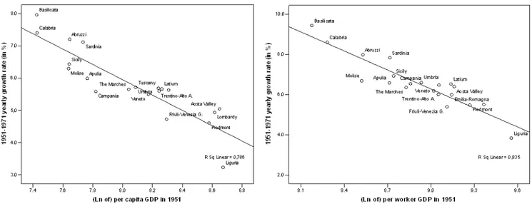
4.3. The golden age (1951-1971)

The graph of beta convergence for the golden age (see Figure 5) is, in many respects, specular to that for the previous period. It is a picture of convergence, in both income and productivity, and of a strong one (standardized beta is -0.886 for per capita GDP, -0.914 for per worker GDP). Furthermore, it is worth noticing as, at least in income, we have once again the threefold repartition: all the regions of South and islands are at the top (they grow the most), all those of the North-East and Centre in the middle, all those of the North-West at the bottom. In productivity, we observe something similar, the only difference being that in this case the three-fold repartition is a bit less defined. To be more precise, it should be added that the convergence in per capita GDP is entirely driven by productivity in the case 15 _{For an updated analysis of economic and social policies in Fascist Italy, see Felice (2015b, pp. 186-227).}

of southern Italy – which indeed, as average, slightly fell behind in workers per capita (see Table 3). For the NEC regions the contribution of productivity is less strong, only in part counterbalanced by the fact that there is no falling behind in workers per capita.

Such a convergence process is an exception in the entire history of post-unification Italy: it did not happen before, it won’t happen again. Furthermore, it took place during the period of most intense growth of the Italian economy, that is when also the leading North-West was growing as never before – and for this reason, it seems at odds with theoretical predictions (both those from the neo-classical approach and the alternative new economic geography). How can be explained? On the one end, and this is true for the North-East and Centre, there is the beginning of a diffusive process seeing the spread of industry towards the bordering regions of the Triangle, such as Emilia-Romagna, Veneto, Tuscany, and then the Marches (Fuà e Zacchia, 1983; Bagnasco, 1988; Bellandi, 1999); this process, however, will gain momentum only from the 1970s onwards, that is, after the crisis of the big firms more intensive in energy and capital (and in fact the convergence of the NEC is relatively mild during the golden age). On the other end, and here is the most important factor, there is the Italian state actively intervening in the South, to promote first infrastructures and then industrialization – and therefore strongly altering the market rules (upon which also the competing theories are based) in favor of the convergence of the most backward regions (Felice, 2007a, pp. 72-93). From 1957 until the mid 1970s, the state-owned Cassa per il Mezzogiorno financed in the South new plants in capital-intensive and highly productive industrial sectors (steel, chemicals, engineering, electronics), mostly belonging to state-owned firms although at a later stage also to the private big business (Fiat above all) (Felice and Lepore, 2017; Felice, Lepore and Palermo, 2016): and in fact the South is converging not only in the share of industrial employment, but also – and at a very impressive and high rate – in per worker productivity and particularly in industrial productivity (see the figures in the statistical appendix).16 _{For the first time,}

industrialization is taking place on a massive scale in the South, and it is the modern industry (Svimez, 1971; Del Monte and Giannola, 1978); for the most part, however, it is not a home-grown industry, unlike in the North-East and Centre.

4.4. A tale of two Italies (1971-2011)

The picture for the last period (see Figure 6) is, once again, dramatically different from the previous one – as from that of any other period. It is an entirely distinct scenario. First, there is a remarkable differentiation between per capita and per worker GDP, without precedents: in per capita GDP there is, practically, no longer convergence (standardized beta is down to -0.048); conversely, in per worker GDP convergence continues, with quite a high value for standardized beta (-0.865). Second, and more precisely, the lack of convergence in per capita GDP is limited to the southern regions: those that grew the most in the previous decades (but that still lie behind in absolute terms) are now falling behind. Conversely, the 16 _{Internal migration, from the South to the North, may also have played some role, but probably a minor one;}

actually, in this period the South fell back in terms of activity rates, and thus it could be argued that emigration could have been even negative, drawing away the most productive labour force; in any case, what caused convergence in per capita GDP was the growth of southern employment in industry and services, and the fact that this employment produced high GDP per worker.

NEC regions – plus the small northernmost regions of the South, Abruzzi and Molise – continue to converge: this is patent in the left part of Figure 6, where we observe all these regions above the fit line; while all the other southern regions are below, in the left, and most of the North-West is also below, in the right. As a consequence of this process, as we have seen by the early twenty-first century Italy looks divided into two parts: a Centre-North much more homogeneous internally, as never before, and a poorer South. Convergence was half-completed, we could say, that is it was (more or less) achieved for one of the two macro-areas behind the North-West. But it was half-convergence also because, for the South, it actually continued in one of the two components of per capita GDP: productivity. Here nowadays a gap is still present, but it is also true that southern Italy converged, slowly nonetheless, reaching 90% of the Italian average. Of course you can see the glass half empty: there is, in this period, a dramatic falling back of southern Italy in employment (ten points are lost over the Italian average in forty years, down to 77% of the Italian average, see Table 3): the underdevelopment of southern Italy is now, essentially, a problem of unemployment.

In a certain sense, the falling behind of southern Italy is the other side of its convergence, in the previous periods: those very capital-intensive plants, that were financed by the State and weaker than analogous plants in the North, collapsed with the oil-shocks (Pontarollo and Cimatoribus, 1992; Barbagallo and Bruno, 1997). At the same time, however, the effectiveness of State intervention in the South went lost, because of growing political clientelism, wrong industrial choices, and even an increasing and at traits pervasive influence of organized crime (e.g. Bevilacqua, 1993, pp. 126-132; Felice, 2013, pp. 112-116 and 149-163). In this respect, the convergence in productivity should not be overestimated, being limited to those who work (of course), and being artificially prompted by national laws, who set wages equal throughout the country,17 thus leveling per worker GDP figures independently of real productivity (furthermore, in some tertiary sectors of growing importance, such as public administration, ‘real’ productivity cannot even be measured) (Fuà, 1993). To all of this, in sharp contrast stands the convergence of the North-East and Centre: it is a convergence of ongoing industrialization, led by small and later on by medium sized firms, at first organized in industrial districts (Becattini, 1979, 1987; Saba, 1995),18

then evolving in the so-called ‘fourth capitalism’ (medium sized, highly international firms emerging from their former districts) (Colli, 2002, 2003).19 In line with the post-Fordist scenario, the relevant sectors are, broadly speaking, light manufactures intensive in labor, and this explains why the NEC performs much better in workers per capita than in productivity – once again, the opposite of South and islands.

5. In guise of a conclusion: where do we go from now?

From this broad picture, can we draw some conclusions – or at least, can we develop hypotheses – about the determinants of regional inequality in Italy over the long-run? We 17 _{A territorial wage differentiation (the so-called gabbie salariali) was introduced in 1945, but abolished in}

1969. The subject reemerged in the political and economic debate of the country in the following decades. For a brief overview, see Busetta and Sacco (1992).

18 _{On the social and economic characteristics of the so-called ‘third Italy’, see also Bagnasco (1977) and}

Trigilia (1986).

19 _{The expression was first introduced in Turani, 1996, p. 125.}

have seen, in the previous section, as the new figures fit quite well with (some of) the vast literature about regional development in Italy. But if in terms of description we have made significant steps, for what concerns the interpretation, the research still has a long road ahead. Recent works allow us to discuss the role of geography – the market size, in particular – following the approach of the new economic geography (Krugman, 1991); as well as other crucial determinants such as human and social capital, which can be treated as conditioning variables following the alternative neo-classical conditional convergence (Barro and Sala-i-Martin 1992, 2004) and the well-known augmented Solow model framework.20 None of them (neither alone, nor in combination)21 seems to be, thus far, the key explanatory factor of Italy’s regional inequality in the long-run: an obvious impediment is posed by the fact that the history of regional inequality in post-unification Italy is not uniform, as we have seen, but structured around historical periods quite different from each other. But it is not only this, as we are going to explain.

The most updated estimates for the market size suggest that this did not play a major role in the liberal age (Missiaia, 2016). For the second half of the twentieth century, although the debate is open (A’Hearn and Venables, 2013), the basic conclusion should not be different: geography is likely not to be the major ingredient behind the falling back of the Mezzogiorno. Against the importance of geography, is the fact that Campania, the most geographically favored region of the South (and one that in terms of market size was above the Italian average), actually is the region with the worst performance in the South and in the entire country; in a specular way, other regions not favored in terms of market size, namely the mountainous Trentino-Alto Adige or Aosta Valley, are the best performers. Apparently against the geographical explanation is also the fact that the falling back of the South in the last four decades is not due to productivity or wage differentials (the primary factor of divergence according to the new economic geography, based on economies of scale favouring divergence and then on costs of congestion favouring convergence) but, instead, to employment: it is a problem of entrepreneurship (in the supply side), not of less productive enterprises for the lack of economies of scale (in the demand side) – and actually the southern regions nowadays are more consumption hubs, than centers of production. This is, however, an issue deserving further investigation, for instance by properly differentiating between the changes in per capita GDP attributable to industry-mix and those attributable to productivity.22 Geography, of course, may have had some role in the performance of particular regions (for instance, although not alone (Felice, 2007b), in the moderate convergence of Abruzzi and Molise during the last decades, once they were connected to Rome through highways); proximity to the European core may have favored the Centre-North in the second half of the twentieth century, after the onset of the Common market (A’Hearn and Venables, 2013) (but in the 1960s southern Italy lived through an impressive convergence); and natural endowments (namely the hydraulic force), more than the market size, have surely played a role in the initial take-off of the northern regions during the liberal age (Cafagna, 1965, 1999). But on the whole, a the present stage of the research this is too little to say that geography was the key factor behind the rise of the North-West, 20 _{See also Durlauf, Johnson and Temple (2005) for a thorough survey (up to 2005, of course) of empirical}

applications.

21 _{For a useful combination of both these approaches, see Midelfart-Knarvik, Overman and Venables (2000).}

For an application to Spain, see Martínez-Galarraga (2012).

22 _{For an application to Spain, see Rosés et al., 2010.}

the convergence of the NEC (mostly in workers per capita), the falling back of the South (equally in workers per capita); at best, it could have been a concomitant factor.

Long-term conditional convergence tests, made on these estimates from 1891 to 2001 at historical borders, suggest that neither human capital, nor social capital are able to explain the falling back of southern Italy. Truly, human capital has played a major role in the first two periods of our story (the liberal age and the interwar years), social capital in the last one (Felice, 2012). But none of them, and not even a combination of the two, seem to be the key conditioning variable in the long-run: a model with fixed effect (which are negative in the South) remain superior even after the introduction of both the conditioning variables – and regressions run with the present estimates, which only add a few more benchmarks, and some more cases for the regions at current borders, would yield similar results. So, what are the unexplained fixed effects which hampered the convergence of the South? (and, more in particular, its structural change and growth of activity rates?) It has been argued that these fixed effects could be enduring socio-institutional differences: higher inequality in the South, coupled with extractive political (clientelism) and economic (latifundium versus sharecropping, organized crime) institutions, which reinforced a de facto extractive setting in the South – although within a nominally national institutional framework (Felice, 2013). Historically, inequality and extractive institutions in the South may have also determined, in that area, lower human and social capital, that is, they may have created the concomitant conditioning variables which favored the falling back of the South in some periods; furthermore, we know that in the 1970s they caused the collapse of the regional policies and the deteriorating of State intervention, which marked the end of convergence in that decade and the ensuing slowly falling back. This hypothesis is fascinating, and quite in line with the evolution of regional inequality we have reconstructed in this article, but it still lacks a rigorous quantitative testing; in part, this is due to the fact that it is not easy to properly quantify a de facto functioning of institutions (most of them are nominally the same) – and it is even more difficult to do so for past historical periods.

Nevertheless, it is a challenge worth being taken on. Surely, results would be much more reliable if we were able to pass from regional (NUTS II level) to provincial (NUTS III) estimates of GDP and productivity. Provincial estimates are on their way to be produced, at least for the industrials sector (Ciccarelli and Fenoaltea, 2012c; Ciccarelli, 2015) (but those for the services and agriculture should be equally feasible), and therefore it would not be impossible to have, for the future, a picture at the provincial level similar to the regional one we have presented in this article. Provincial figures would remarkably increase the robustness of conditional convergence tests, at least for specific periods, thus giving us better insights on the roles played by human and social capital (for both variables too, figures can be produced at the provincial level), as well as by natural endowments. At the provincial level, and at least for specific periods, even estimates of institutional functioning and differences, to be profitably tested into models, could be produced: for instance, for what concerns agrarian regimes (hard to be generalized at the regional level), or the historical presence of organized crime in specific territories of the South (Buonanno et al., 2015), or election corruption and cronyism. The overall picture – the broad pattern of territorial inequality in the long run – would not change; it may instead significantly improve the interpretation.

Figure 1. The Italian regions at historical borders (1871-today)

Figure 2. Beta and sigma convergence in per capita GDP, per worker GDP and workers

per capita, 1871-2011

Notes and sources: elaborations from tables 1-3; for beta convergence, standardized beta is -0.497 for per capita GDP, -0.893

for per worker GDP, -0.166 for workers per capita; sigma convergence is the Williamson index, that is, it is calculated using as

weights the regional shares of population, according to the formula: , where y is the per capita GDP, p is the population and i and m refer to the i-region and the national total, respectively (Williamson, 1965).

Figure 3. Beta convergence in per capita and per worker GDP, 1871-1911

Notes and sources: elaborations from tables 1-2; standardized beta is -0.183 for per capita GDP, -0.224 for per

worker GDP.

Figure 4. Beta convergence in per capita and per worker GDP, 1911-1951

Notes and sources: elaborations from tables 1-2; standardized beta is 0.259 for per capita GDP, 0.072 for per

worker GDP.

Figure 5. Beta convergence in per capita and per worker GDP, 1951-1971

Notes and sources: elaborations from tables 1-2; standardized beta is -0.886 for per capita GDP, -0.914 for per

worker GDP.

Figure 6. Beta convergence in per capita and per worker GDP, 1971-2011

Notes and sources: elaborations from tables 1-2; standardized beta is -0.048 for per capita GDP, -0.865 for per

Tab le 1 . P er c api ta G D P of the It al ian r egi ons , 1871-2011 (It al y = 100 ) 187 1 188 1 189 1 190 1 191 1 192 1 193 1 193 8 195 1 196 1 19 71 198 1 199 1 200 1 201 1 Pi edm ont 107 108 107 119 116 128 123 138 151 131 124 119 114 115 109 Ao st a Val le y 80 99 106 119 129 143 143 144 158 168 144 140 142 124 136 Li gu ria 138 142 139 148 157 142 164 167 162 125 104 101 106 109 106 Lom ba rdy 114 115 114 123 118 124 123 138 153 145 136 130 132 130 129 Tr en tin o-Al to A. 69 73 78 82 78 88 92 94 105 101 107 127 130 130 129 Ven et o 106 89 81 84 88 78 073 83 98 97 98 109 112 113 115 Fr iu li-Ven ezi a G. 125 123 122 125 128 106 117 123 111 91 95 97 104 112 113 Em ili a-R om ag na 96 107 106 102 109 110 109 104 112 117 114 130 122 123 122 Tu scan y 106 108 103 93 098 104 106 101 105 105 108 111 105 109 109 Th e M ar ch es 83 78 88 83 082 78 71 78 86 87 88 100 95 99 102 U mb ria 99 103 106 100 092 93 100 95 90 93 93 101 96 96 92 La tiu m 134 145 137 135 133 136 140 119 107 111 110 106 114 113 113 Ab ru zzi 80 77 68 67 70 72 62 57 58 72 79 85 90 85 85 M ol is e 80 77 67 65 68 72 64 59 57 67 66 76 78 80 78 C am pan ia 109 101 99 96 96 88 81 81 69 72 70 65 66 65 64 A pu lia 89 95 104 94 87 92 85 72 65 71 71 67 68 67 68 B as ili ca ta 67 63 75 73 74 75 70 57 46 64 73 69 67 73 71 C al ab ria 69 66 68 66 71 61 55 49 47 59 66 62 62 64 65 Si ci ly 95 92 95 89 87 72 82 72 58 61 69 72 72 66 66 Sa rd in ia 77 81 97 91 93 91 85 82 63 75 85 75 77 77 77 N ort h-We st 114 115 114 125 122 128 129 142 154 138 129 123 124 124 121 N ort h-Ea. & C en . 100 101 99 97 98 101 102 100 104 104 105 112 112 113 114 Sout h & is la nds 90 88 90 86 85 79 77 70 61 68 71 69 70 68 68 C en tre -N ort h 106 107 106 108 108 112 113 117 123 118 115 116 117 117 117 Ita ly (2011 e ur os ) 2049 2225 2327 2562 2989 2843 3506 3853 4813 8158 13268 18202 23141 27113 26065 No te s: t he N or th -W es t c om pr is es P ie dm on t, A os ta V alle y, L ig ur ia , L om ba rd y; th e N or th -E as t a nd C en tre c om pr is e T re ntin o-A lto A di ge , V ene to , F riul i-V en ez ia G iu lia , E m ilia -R om ag na, T us can y, T he Mar ch es , U m br ia, L at iu m ; A br uzzi , M ol is e, C am pa ni a, A pu lia, B as ili cat a, C al ab ria, S ici ly a nd S ar di ni a ar e t he r eg io ns o f s ou th er n I ta ly; t he C ent re -N or th i s m ade of t he N or th -W es t a nd t he N or th -E as t an d C en tre. S ee al so F ig ur e 1 . Sour ce s: s ee Se ct io n 2 an d, fo r f ur th er d et ai ls , t he A pp en di x. T he n at io nal fi gu res ar e f ro m F el ice an d V ecch i ( 2015a ). 25

Ta bl e 2. Per w or ker G D P o f t he It al ian r egi ons , 1871-2011 (It al y = 100 ) 187 1 188 1 189 1 190 1 191 1 192 1 193 1 193 8 195 1 196 1 197 1 198 1 199 1 200 1 201 1 Pi edm ont 103 94 93 105 99 106 102 114 124 112 108 107 105 105 99 Ao st a Val le y 71 83 83 90 90 101 88 98 111 130 115 106 111 102 109 Li gu ria 134 136 135 147 152 142 157 160 165 125 105 101 105 107 104 Lom ba rdy 109 100 102 113 111 114 110 125 137 127 119 116 113 113 115 Tr en tin o-Al to A. 53 67 71 79 69 84 86 86 100 90 96 102 105 104 105 Ven et o 115 92 83 86 88 81 78 84 97 95 96 100 99 99 98 Fr iu li-Ven ezi a G. 94 106 108 115 98 145 136 112 106 86 91 89 97 101 100 Em ili a-R om ag na 93 107 105 99 105 104 104 95 109 110 105 110 103 103 101 Tu scan y 102 109 104 94 97 105 102 98 100 99 105 101 97 98 99 Th e M ar ch es 76 71 81 77 77 71 64 71 80 78 82 86 87 93 89 U mb ria 90 103 106 101 91 90 98 91 89 91 95 98 95 94 89 La tiu m 123 139 135 136 137 140 140 121 109 118 115 113 113 109 108 Ab ru zzi 83 76 65 62 67 69 66 58 59 74 82 89 94 89 91 M ol is e 81 76 65 62 67 69 67 58 59 52 64 78 90 89 83 C am pan ia 106 104 101 97 98 91 89 93 82 87 87 79 87 88 92 A pu lia 94 106 114 103 95 102 98 84 71 78 76 80 81 82 87 B as ili ca ta 73 64 73 68 70 69 73 57 42 61 75 77 86 90 81 C al ab ria 72 75 69 60 67 58 62 54 46 66 72 75 79 82 82 Si ci ly 104 108 114 108 106 89 98 91 73 77 84 93 94 90 91 Sa rd in ia 94 100 119 111 113 112 95 97 71 86 97 91 86 88 86 N ort h-We st 109 102 103 114 112 115 113 126 136 123 114 111 110 110 109 N ort h-Ea. & C en . 99 103 101 99 99 103 101 96 101 101 102 104 102 102 101 So ut h & is la nd s 95 97 99 93 93 87 87 82 69 78 82 84 87 87 89 C en tre -N ort h 103 102 102 105 104 108 106 108 115 110 107 107 105 105 104 Ita ly (2011 e ur os ) 6302 6423 7266 8068 9455 8120 10425 11111 15106 22094 35925 46604 55486 64813 65743 Not es and s our ce s: s ee t ab le 1 .

Ta bl e 3. W or ke rs pe r c ap ita of the It al ian r egi ons , 1871-2011 (It al y = 100 ) 187 1 188 1 189 1 190 1 191 1 192 1 193 1 193 8 195 1 196 1 197 1 198 1 199 1 200 1 201 1 Pi edm ont 104 115 115 114 117 121 121 121 119 117 114 111 108 110 110 Ao st a Val le y 112 120 127 132 143 142 162 146 142 129 125 131 128 121 125 Li gu ria 103 105 103 101 103 100 105 104 98 100 99 100 101 103 102 Lom ba rdy 104 114 111 108 106 109 113 110 112 114 114 112 117 115 112 Tr en tin o-Al to A. 130 11 0 110 104 113 104 108 109 106 112 111 124 123 124 123 Ven et o 92 97 98 98 100 97 94 98 102 103 102 109 113 115 117 Fr iu li-Ven ezi a G. 81 73 72 73 74 73 86 110 105 106 105 108 107 111 114 Em ili a-R om ag na 103 99 101 103 104 106 105 109 103 106 109 118 119 12 0 121 Tu scan y 103 99 99 99 102 99 104 103 105 106 103 110 107 111 110 Th e M ar ch es 109 110 109 109 106 111 111 110 108 112 108 117 108 107 114 U mb ria 111 100 101 100 102 103 102 105 102 102 98 103 101 102 103 La tiu m 108 104 102 99 97 97 100 98 99 94 96 94 101 103 105 Ab ru zzi 96 101 104 108 104 105 94 99 98 96 97 96 96 96 93 M ol is e 99 101 102 104 102 104 96 102 98 128 104 98 87 90 93 C am pan ia 102 98 98 99 99 97 91 87 84 82 80 82 76 74 70 A pu lia 95 90 91 91 92 90 86 85 92 91 93 84 83 81 78 B as ili ca ta 92 98 103 107 107 109 96 100 112 106 97 90 78 81 87 C al ab ria 96 89 98 111 106 106 90 91 101 90 92 83 78 78 79 Si ci ly 91 85 83 82 81 81 84 79 79 80 82 78 76 74 73 Sa rd in ia 82 81 82 82 83 81 90 85 89 88 88 83 89 87 90 N ort h-We st 104 114 112 110 110 112 115 113 112 113 112 111 113 112 111 N ort h-Ea. & C en . 102 99 99 99 100 99 101 104 103 103 103 108 110 112 113 Sout h & is la nds 95 92 93 94 93 92 89 87 89 87 87 83 80 79 77 C en tre -N ort h 103 105 104 103 104 104 106 107 107 107 107 109 111 112 112 Ita ly (% ) 45, 2 50, 3 49, 8 49, 7 47, 0 47, 2 39, 8 43, 4 42, 2 41, 9 37, 1 39, 1 41, 6 41, 7 39, 6 Not es and s our ce s: s ee ta ble 1 . E st im at es ar e b as ed o n t he p re se nt p op ula tio n. 27

References

A’Hearn, B., Venables, A.J. (2013). “Regional Disparities: Internal Geography and External Trade”. In Toniolo, G., (ed.): The Oxford Handbook of the Italian Economy Since Unification. Oxford: Oxford University Press, 599-630.

Aguilar-Retureta, J. (2015). “The GDP per capita of the Mexican regions (1895-1930): new estimates”. Revista de Historia Económica/Journal of Iberian and Latin American Economic

History, 33, n. 3, 387-423.

Ardeni, P.G., Gentili, A. (2014). “Revisiting Italian emigration before the Great War: a test of the standard economic model”. European Review of Economic History, 18, n. 4, 452-471.

Badià-Miró, M. (2015). “The evolution of the location of economic activity in Chile in the long run: a paradox of extreme concentration in absence of agglomeration economies”. Estudios de Economía, 42, n. 2, 143-167.

Badià-Miró, M., Guilera, J., Lains, P. (2012). “Regional Incomes in Portugal: Industrialization, Integration and Inequality, 1890-1980”. Revista de Historia Económica/Journal of Iberian

and Latin American Economic History, 30, n. 2, 225-244.

Baffigi, A. (2011). “Italian National Accounts, 1861-2011”. Bank of Italy, Economic History

Working Papers, 18.

——— (2015). Il PIL per la storia d’Italia. Istruzioni per l’uso. Venezia: Marsilio.

Bagnasco, A. (1977). Tre Italie. La problematica territoriale dello sviluppo italiano. Bologna: il Mulino.

——— (1988). La costruzione sociale del mercato. Studi sullo sviluppo di piccola impresa in Italia. Bologna: il Mulino.

Barbagallo, F., Bruno, G. (1997). “Espansione e deriva del Mezzogiorno”. In Barbagallo, F. (ed.):

Storia dell’Italia repubblicana, vol. III. L’Italia nella crisi dell’ultimo ventennio. 2. Istituzioni, politiche, culture. Turin: Einaudi, 399-470.

Barro, R.J., Sala-i-Martin, X. (1992). “Convergence”. Journal of Political Economy, 100, n. 2, 223-251.

——— (2004). Economic Growth. Second edition. Cambridge (MA): Massachusetts Institute of Technology.

Battilani, P. (2001). Vacanze di pochi, vacanze di tutti. L’evoluzione del turismo europeo. Bologna: il Mulino.

Becattini, G. (1979). “Dal ‘settore’ industriale al ‘distretto’ industriale. Alcune considerazioni sull’unità di indagine dell’economia industriale”. Rivista di economia e politica industriale, 5, n. 1, 7-21.