The PVLAS experiment: A 25 year effort to measure vacuum magnetic birefringence

Contents lists available atScienceDirect

Physics Reports

journal homepage:www.elsevier.com/locate/physrep

The PVLAS experiment: A 25 year effort to measure vacuum

magnetic birefringence

A. Ejlli

a

, F. Della Valle

b,c

, U. Gastaldi

d

, G. Messineo

e

, R. Pengo

f

, G. Ruoso

f

,

G. Zavattini

d,g,∗

a_{School of Physics and Astronomy, Cardiff University, Queen’s Building, The Parade, Cardiff CF24 3AA, United Kingdom} b_{Dip. di Scienze Fisiche della Terra e dell’Ambiente, via Roma 56, I-53100 Siena, Italy}

c_{INFN - Sez. di Pisa, Largo B. Pontecorvo 3, I-56127 Pisa, Italy} d_{INFN - Sez. di Ferrara, Via G. Saragat 1, I-44100 Ferrara, Italy} e_{Department of Physics, University of Florida, Gainesville, FL 32611, USA}

f_{INFN - Laboratori Nazionali di Legnaro, Viale dell’Università 2, I-35020 Legnaro, Italy} g_{Dip. di Fisica e Scienze della Terra, Via G. Saragat 1, I-44100 Ferrara, Italy}

a r t i c l e i n f o

Article history:

Received 3 March 2020

Received in revised form 29 May 2020 Accepted 2 June 2020

Available online 10 June 2020 Editor: Jonathan L. Feng

a b s t r a c t

This paper describes the 25 year effort to measure vacuum magnetic birefringence and dichroism with the PVLAS experiment. The experiment went through two main phases: the first using a rotating superconducting magnet and the second using two rotating permanent magnets. The experiment was not able to reach the predicted value from QED. Nonetheless the experiment has set the current best limits on vacuum magnetic birefringence and dichroism for a field of Bext=2.5 T, namely,∆n(PVLAS)=(12±17)×

10−23_and|∆κ|(PVLAS)_{=(10±28)×10}−23_{. The uncertainty on∆n}(PVLAS)_{is about a factor}

7 above the predicted value of∆n(QED)_=2.5×10−23_{@ 2.5 T.}

© 2020 The Authors. Published by Elsevier B.V. This is an open access article under the CC BY license (http://creativecommons.org/licenses/by/4.0/).

Contents

1. Introduction... 3

2. Theoretical considerations... 4

2.1. Classical electromagnetism... 4

2.2. Light-by-light interaction at low energies... 5

2.2.1. Leading order vacuum birefringence and dichroism in electrodynamics... 7

2.2.2. Higher order corrections... 9

2.2.3. Born–Infeld... 9

2.3. Axion like particles... 10

2.4. Millicharged particles... 11

2.5. Chameleons and dark energy... 12

3. The experimental method... 12

3.1. Polarimetric scheme... 12

3.2. The Fabry–Perot interferometer as an optical path multiplier... 15

3.3. Fabry–Perot Systematics... 17

3.3.1. Phase offset and cavity birefringence... 17

3.3.2. Frequency response... 19

∗

Corresponding author at: Dip. di Fisica e Scienze della Terra, Via G. Saragat 1, I-44100 Ferrara, Italy.

E-mail address: zavattini@fe.infn.it(G. Zavattini). https://doi.org/10.1016/j.physrep.2020.06.001

0370-1573/©2020 The Authors. Published by Elsevier B.V. This is an open access article under the CC BY license (http://creativecommons.org/ licenses/by/4.0/).

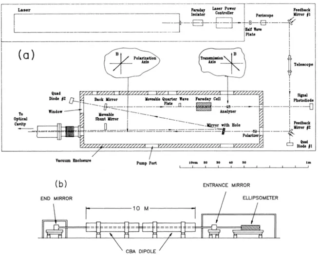
3.4. CaLibration... 20 3.5. Noise budget... 22 3.6. Gravitational antennae... 24 4. PVLAS Forerunners... 25 4.1. CERN Proposal: 1980–1983... 26 4.2. BFRT: 1986–1993... 27 4.3. PVLAS-LNL: 1992–2007... 29 4.3.1. Infrastructures... 30 4.3.2. Superconducting magnet... 31 4.3.3. Rotating cryostat... 31 4.3.4. Fabry–Perot Cavity... 31 4.3.5. Results... 32 4.4. PVLAS-Test: 2009–2012... 33

5. The PVLAS-FE experiment... 34

5.1. Summary... 34

5.2. General description of the apparatus... 34

5.3. Optical bench and vibration isolation... 35

5.4. Vacuum system... 36

5.5. Vacuum tubes through the magnets... 37

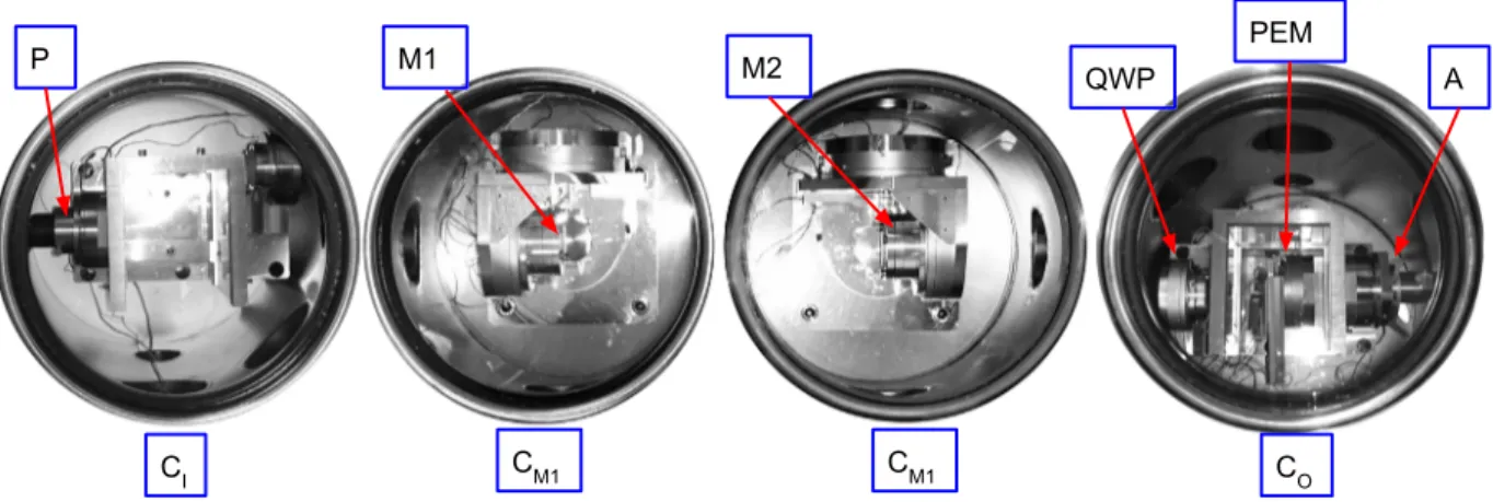
5.6. Optical vacuum mounts... 38

5.7. The rotating permanent magnets... 38

5.8. The Fabry–Perot cavity... 39

5.9. Data acquisition... 41

5.10. Data analysis... 41

6. PVLAS-FE commissioning... 42

6.1. Calibration measurements... 42

6.1.1. Characterisation of the cavity birefringence... 42

6.1.2. Frequency response measurements... 44

6.1.3. Cotton–Mouton measurements... 45

6.1.4. Faraday effect measurements... 46

6.2. In-phase spurious signals... 46

6.2.1. Stray fields and pick-ups... 46

6.2.2. Mechanical noise from the rotating magnets... 48

6.2.3. Movements of the optical bench... 49

6.2.4. Diffused light and ‘in-phase’ spurious peaks... 50

6.2.5. Magnetic forces on the tube... 51

6.2.6. ‘In-phase’ spurious signals conclusion... 52

6.3. Wide band noise... 53

6.3.1. Diffused light and wide band noise... 53

6.3.2. Ambient noise... 53

6.3.3. The role of the finesse... 55

6.3.4. Ellipticity modulation... 56

6.3.5. Cavity frequency difference for the two polarisation states... 57

6.3.6. Power induced noise... 59

6.3.7. Intrinsic noise... 59

6.3.8. Final discussion on wide band noise: thermal noise issues... 61

6.4. Conclusions on the commissioning: lessons learned... 63

7. Measurements of the vacuum magnetic birefringence and dichroism... 64

8. Vacuum measurement results and time evolution... 65

8.1. Limits on vacuum magnetic birefringence and dichroism... 65

8.2. Limits on hypothetical particles... 66

8.2.1. Axion like particles... 66

8.2.2. Millicharged particles... 68

9. Conclusions... 68

Declaration of competing interest... 69

Acknowledgements... 69

1. Introduction

The velocity of light in vacuum is considered today to be a universal constant and is defined as c

=

299 792 458 m

/

s in the International System of Units:

c

=

1

√ε

0

µ

0

.

(1)

It is related to the vacuum magnetic permeability

µ

0and the vacuum permittivity

ε

0which describe the properties of classical electromagnetic vacuum.1Classically this relation derives directly from Maxwell’s equations in vacuum. Due to their linearity c does not depend on the presence of other electromagnetic fields (photons, static fields).

Today Quantum Electrodynamics (QED) describes electrodynamics to an incredibly accurate level having been tested in many different systems at a microscopic level: (g

−2)

e,µ[1,2], Lamb-shift [3], Delbrück scattering [4] etc. One fundamental

process predicted since 1935 [5–7] (before the formulation of QED), namely 4-field interactions with only photons present in both the initial and final states, still needs attention. In the above mentioned measurements either the accuracy is such that the 4-field interaction must be taken into account as a correction to the first order effect being observed or, as is the case of Delbrück scattering, this contribution must be distinguished from a series of other effects. The 4-field interaction considered to first order will lead to two effects: light-by-light (LbL) scattering and vacuum magnetic (or electric) linear birefringence (VMB) due to low energy coherent Delbrück scattering. This first effect occurs at a microscopic level whereas VMB describes a macroscopic effect related to the index of refraction [8–12] and is a direct manifestation of quantum vacuum. In recent years, with the ATLAS and CMS experiments at the LHC collider, LbL scattering at high energies has been observed [13–15] via

γ γ

pair emission during Pb-Pb peripheral collisions forh

¯

ω ≫

mec2. Furthermore, optical

polarimetry of an isolated neutron star has led Mignani et al. to publish evidence of VMB [16].

It remains that this purely quantum mechanical effect still needs a direct laboratory verification in the low energy regime,

¯

h

ω ≪

mec2, at the macroscopic level.

As will be discussed in the following sections, not only does the index of refraction depend on the presence of external fields but it depends also on the polarisation direction of the propagating light. In the presence of an external magnetic field perpendicular to the propagation direction of a beam of light, one finds

{

n∥⃗B

=

1

+

7AeB2ext n_⊥⃗B

=

1

+

4AeB2ext

(2) where the subscripts (∥ ⃗B) and (

⊥ ⃗

B) indicate the polarisation direction with respect to the external field. Similarly, in the presence of an electric field

{

n∥⃗E

=

1

+

4AeEext2

/

c2 n⊥⃗E

=

1

+

7AeEext2

/

c2

.

(3) As will be discussed in Section2, the parameter Ae describes the non linearity of Maxwell’s equations due to vacuum

fluctuations: Ae

=

2 45

µ

0

¯

h3 m4 ec5

α

2

₌

₁

_.

₃₂

_×

₁₀−24_T−2 ₍₄₎

where

α

is the fine structure constant, and methe mass of the electron.

The first modern proposal to measure QED non-linearities due to vacuum polarisation at very low energies dates back to 1979 [17] and a first attempt was performed at CERN during the beginning of the ’80s to study the feasibility of such a measurement. Since then the idea to detect the induced birefringence due to an external magnetic field using optical techniques has been an experimental challenge. Optical elements and lasers have since improved tremendously but as of today, in spite of the unceasing efforts [18–21], the direct measurement of VMB is still lacking. Another ongoing attempt to tackle the same physics is in Ref. [22]: detecting the refraction of light-by-light in vacuum is their goal. Searches for direct photon–photon elastic scattering are reported in Refs. [23,24]. Note that heuristic approaches to this very same matter started before and prescinded from any theoretical justification [25–31]. More literature and a general treatment of non linear vacuum properties can be found in Ref. [32].

Following two precursor experiments, the one at CERN and the other at the Brookhaven National Laboratories (BNL) briefly described in Sections4.1and4.2, the PVLAS (Polarizzazione del Vuoto con LAser) experiment, financed by INFN (Istituto Nazionale di Fisica Nucleare, Italy), performed a long lasting attempt starting from 1993. This experiment went

1 _{Today (after the redefinition of the SI system on May 20}th_{2019) the values ofε}

0andµ0are both derived from the measurement of the fine structure constant α = e2 4πε0hc¯ =e 2_cµ 0 4π ¯h

through two major phases: the first with a rotating superconducting magnet and the second with two rotating permanent magnets.

In this paper we will describe at length the 25 year development of the PVLAS experiment and present the final results which represent today the best limit on VMB, closest to the expected value determined in Eqs.(2). In the description of the various phases of the experiment many details are given which generally are excluded in scientific papers. We believe this is an opportunity to gather all this information together in a single publication. The last three years of activity of PVLAS coincided with the PhD thesis of one of the authors. More details on the experiment can be found in that work [33].

In Section2we will present the physics related to PVLAS including the possibility of searching for physics beyond the Standard Model. In Section3we will describe the general experimental method of the experiment including systematic effects. In Section4each attempt with its peculiarities will be described: there we will discuss the limitations of each effort and the results obtained. Finally in Sections6–8we will present the calibration method, systematics-hunting, noise issues and results of the last phase of the PVLAS experiment.

2. Theoretical considerations

2.1. Classical electromagnetism

Maxwell’s equations in a medium are given by

⃗

∇ · ⃗

D

=

ρ

∇ × ⃗

⃗

E

= −

∂⃗

B

∂

t

⃗

∇ · ⃗

B

=

0

∇ × ⃗

⃗

H

= ⃗

J

+

∂ ⃗

D

∂

t (5)

where E and

⃗

B are respectively the electric field and the magnetic induction,

⃗

D and

⃗

H are respectively the electric

⃗

displacement field and the magnetic intensity and

ρ

and

⃗

_{J are the free charge density and free current density. The} relations betweenE and

⃗

D and between

⃗

B and

⃗

H are given by

⃗

⃗

D

=

ε

0E

⃗

+ ⃗

P H

⃗

=

⃗

B

µ

0

− ⃗

M (6)

where

⃗

P andM are the polarisation and magnetisation vectors, respectively, with which one can describe the polarisation

⃗

and magnetisation properties of the medium.

These equations can be derived from the Lagrangian densityL_Mattin matter

LMatt

=

1 2

µ

0

(

E2 c2

−

B 2

)

+ ⃗

E

· ⃗

P

+ ⃗

B

· ⃗

M

−

ρϕ + ⃗

J

· ⃗

A (7)

by applying the Euler–Lagrange equations

∂

∂

t

∂

LMatt

∂

(

∂

qi

∂

t

)

+

3

∑

k=1

∂

∂

xk

∂

LMatt

∂

(

∂

qi

∂

xk

)

−

∂

LMatt

∂

qi

=

0

.

(8)

The generalised coordinates q0

=

ϕ

and q1,2,3

= ⃗

A are the scalar and vector potentials, and the fieldsE and

⃗

⃗

B are defined as

⃗

E

= − ⃗

∇

ϕ −

∂⃗

A

∂

t (9)

⃗

B

= ⃗

∇ × ⃗

A

.

(10)

Considering first of all q0

=

ϕ

, Eqs. (8)lead to

⃗

∇ ·

(ε

₀

⃗

E

+ ⃗

P

)

=

ρ

(11)

from which we defineD

⃗

=

ε

₀E

⃗

+ ⃗

P. Similarly by applying Eqs. (8)with respect to q1

=

Ax one finds

⎡

⎣

∂(ε

0E

⃗

+ ⃗

P

)

∂

t

− ⃗

∇ ×

(

1

µ

0

⃗

B

− ⃗

M

)

⎤

⎦

x

= ⃗

Jx (12)

and idem for q2and q3. We can then also defineH

⃗

=

_µ01

⃗

B

− ⃗

M.

In the absence of matter, free charges and currents, resulting in_P

⃗

₌

_0,M

⃗

₌

_0,

⃗

_J

₌

_{0 and}

_{ρ =}

_{0, the Lagrangian density} simplifies to L_Cl

=

1 2

µ

0

(

E2 c2

−

B 2

)

(13) and one finds thatD

⃗

=

ε

₀E and

⃗

⃗

B

=

µ

₀H. Maxwell’s equations in vacuum then become

⃗

⃗

∇ · ⃗

E

=

0

_{∇ × ⃗}

⃗

_E

_{= −}

∂⃗

B

∂

t

⃗

∇ · ⃗

B

=

0

∇ × ⃗

⃗

B

=

ε

₀

µ

₀

∂⃗

E

∂

t

.

(14)

Eqs.(14)admit as solutions electromagnetic waves freely propagating in vacuum at a velocity given by

c

=

1

√ε

0

µ

0

.

(15) Due to the linear behaviour of Maxwell’s equations in vacuum, c does not depend on the presence of external fields.

In general, given a Lagrangian densityL, the vectorsD and

⃗

H can also be determined through the constitutive relations

⃗

⃗

D

=

∂

L

∂⃗

E

⃗

H

= −

∂

L

∂⃗

B (16)

and the polarisation vectorP and magnetisation

⃗

M can be written as

⃗

⃗

P

=

∂

L

∂⃗

E

−

ϵ

₀E

⃗

M

⃗

=

∂

L

∂⃗

B

+

⃗

B

µ

0

.

(17)

2.2. Light-by-light interaction at low energies

This classical scenario changed drastically with the introduction of three new facts at the beginning of the 20th century:

•

Einstein’s energy–mass relationE

=

mc2;

•

Heisenberg’s uncertainty principle∆E∆t

≥ ¯

h

/

2;

•

Dirac’s relativistic equation of the electron admitting negative energy states today identified as anti-matter. These three facts together allow vacuum to fluctuate changing completely the idea of vacuum and allowing for non linear electrodynamic effects in vacuum. Today vacuum is considered as a minimum energy state. Citing from O. Halpern’s letter (1933) [34]

.... Here purely radiation phenomena are of particular interest inasmuch as they might serve in an attempt to formulate observed effects as consequences of hitherto unknown properties of corrected electromagnetic equations. We are seeking, then, scattering properties of the ‘‘vacuum".

In 1935, soon after Halpern’s intuition, two of Heisenberg’s students H. Euler and B. Kockel [7] determined a relativistically, parity-conserving effective Lagrangian density which, to second order in the invariants of the electromagnetic field tensor Fµν (see for example Ref. [35])

F

=

(

B2

−

E 2 c2

)

and G

=

⃗

E c

· ⃗

B

,

(18)

takes into account electron–positron vacuum fluctuations:

LEK

=

LCl

+

Ae

µ

0

⎡

⎣

(

E2 c2

−

B 2

)

2

+

7

( ⃗

_E c

· ⃗

B

)

2

⎤

⎦

(19) where Ae

=

2 45

µ

0

¯

h3 m4 ec5

α

2

₌

₁

_.

₃₂

_×

₁₀−24_T−2

_.

₍₂₀₎

This Lagrangian was derived in the approximation of low energy photonsh

¯

ω ≪

mec2.

The effective Lagrangian densityLEKleads to non linear effects even in the absence of matter thereby violating the superposition principle, one of the building blocks of Maxwell’s theory in vacuum. Indeed by applying the Euler–Lagrange Eqs. (8)with respect to q0

=

ϕ

one obtains

⃗

∇ ·

[

ε

0E

⃗

+

4Ae

(

E2 c2

−

B 2

)

ε

0

⃗

E

+

14

ε

0Ae

(

⃗

E

· ⃗

B

)

⃗

B

]

=

0 (21)

where one can identify

⃗

D

=

ε

₀E

⃗

+

4Ae

(

E2 c2

−

B 2

)

ε

0

⃗

E

+

14

ε

0Ae

(

⃗

E

· ⃗

B

)

⃗

B (22) consistent withD

⃗

=

∂

LEK

∂⃗

E and

⃗

∇ · ⃗

D

=

0. The relation betweenD and

⃗

E is no longer linear in the field

⃗

⃗

E. In a similar way by applying the Euler–Lagrange equations(8)with respect to q1

=

Axone again finds that

∂

Dx

∂

t

−

(

⃗

∇ × ⃗

H

)

x

=

0 (23)

and idem for q2and q3. These equations represent Ampère-Maxwell’s law in a medium where

µ

0H

⃗

= ⃗

B

+

4Ae

(

E2 c2

−

B 2

)

⃗

B

−

14Ae

( ⃗

_E c

· ⃗

B

) ⃗

_E c

.

(24)

Vacuum therefore behaves as a non linear polarisable and magnetisable medium, where_{P and}

⃗

_{M are given by}

⃗

⃗

P

=

4Ae

(

E2 c2

−

B 2

)

ε

0E

⃗

+

14

ε

0Ae

(

⃗

E

· ⃗

B

)

⃗

B (25)

⃗

M

= −4A

e

(

E2 c2

−

B 2

)

_⃗

B

µ

0

+

14Ae

( ⃗

_E c

·

⃗

B

µ

0

) ⃗

_E c

.

(26)

Using the Lagrangian density(19)one can still describe electromagnetism in the absence of matter using Maxwell’s equations but in the form(5): i.e. in a medium which is both magnetised and polarised by an external field due to the presence of virtual electron–positron pairs.

A direct consequence of the non linear behaviour of Eqs.(22)and(24)is that the velocity of light now depends on the presence of external fields in contradiction with Maxwell’s equations in classical vacuum. Given a certain configuration of external fields, for example in whichB

⃗

=

µ

0

µ

(E

⃗

, ⃗

B)H and

⃗

D

⃗

=

ε

0

ε

(

⃗

E

, ⃗

B)E, the index of refraction n is

⃗

n

=

√

εµ ̸=

1

.

(27)

To summarise, vacuum fluctuations determine the following important facts:

•

in vacuumD

⃗

̸=

ε

₀E and

⃗

B

⃗

̸=

µ

₀H;

⃗

•

Maxwell’s equations are no longer linear and the superposition principle is violated;

•

in vacuum Light-by-Light scattering can occur and the velocity of light is

v

light

<

c in the presence of other electromagnetic fields;

•

electromagnetism in vacuum is described by Maxwell’s equations in a medium.

Detecting this manifestation of quantum vacuum fluctuations at a macroscopic level leading to a dependence of the velocity of light on an external field has been the primary goal of the PVLAS experiment.

The effective Lagrangian density(19)was generalised in 1936 by W. Heisenberg and H. Euler [5]. They determined an effective Lagrangian taking into account electron–positron pairs in a non perturbative expression to all orders in the field invariants F and G in a uniform external background field. Furthermore they introduced the idea of a critical electric field

Ecr

=

m2 ec3

¯

he

=

1

.

32

×

10 18_V

_/

_m

_.

₍₂₈₎

This field corresponds to the field intensity whose work over a distance equal to the reduced Compton wavelength of the electron amounts to the rest energy of the electron: for fields above Ecrreal production of electron–positron pairs arises in vacuum [36]. Today Ecris known as the Schwinger critical field. One can also define a critical magnetic field Bcras

Bcr

=

m2 ec2

¯

he

=

4

.

4

×

10 9_T

_.

₍₂₉₎

Furthermore Heisenberg and Euler set the following conditions on the field derivatives

¯

h mec

|∇

E

| ≪

E

,

h

¯

mec2

⏐

⏐

⏐

⏐

∂

E

∂

t

⏐

⏐

⏐

⏐

≪

E (30)

¯

h mec

|∇

B

| ≪

B

,

h

¯

mec2

⏐

⏐

⏐

⏐

∂

B

∂

t

⏐

⏐

⏐

⏐

≪

B (31)

The resulting Heisenberg–Euler effective Lagrangian density for electromagnetic fields in the absence of matter is LHE = 1 2µ0 ( E2 c2−B 2 ) +α ∫∞ 0 e−ξdξ ξ3× ⎧ ⎨ ⎩ iξ2 √ε 0 µ0 ( ⃗ E· ⃗B) cos[ ξ √ C √ε0Ecr ] +conj. cos[ ξ √ C √ε0Ecr ] −conj. +ε0Ecr2+ ξ2 3µ0 ( B2₋E2 c2 ) ⎫ ⎬ ⎭ (32) with C

=

1

µ

0

(

E2 c2

−

B 2

)

+

2i

√

ε

0

µ

0

(

⃗

E

· ⃗

B

) .

(33)

T3he Euler–Kockel Lagrangian density(19)can be obtained from(32)through a second order expansion in the field invariants F and G (see also Ref. [37]).

A few years later, a number of researchers obtained the same effective Lagrangian density from QED [38,39]. 2.2.1. Leading order vacuum birefringence and dichroism in electrodynamics

In general, the index of refraction of a medium is a complex quantity:n

˜

=

n

+

i

κ

. The real part n (known as the index of refraction tout court) determines the velocity of propagation of light in the medium, whereas the imaginary part, known as the index of absorption

κ

, describes the absorption of the medium.

A medium is said to be birefringent if n depends on the polarisation state of the propagating light. Both linear and circular birefringences exist: the first is a birefringence for linearly polarised light whereas the second is a birefringence for circularly polarised light (also know as optical activity). Similarly a medium is said to be dichroic if the index of absorption

κ

depends on the polarisation (both linear and circular).

Consider a linearly polarised beam of light propagating along a directionk through an external field perpendicular to

ˆ

ˆ

k. The relative dielectric constant and relative magnetic permeability will be obtained from Eqs.(22)and(24)where the electric and magnetic fieldsE and

⃗

⃗

B are the sum of the external fields,

⃗

EextandB

⃗

ext, and the light fieldsE

⃗

γ andB

⃗

γ. In the

case of an external magnetic field

⃗

Bextone hasE

⃗

= ⃗

Eγ and

⃗

B

= ⃗

Bext

+ ⃗

Bγ. Furthermore, considering the case in which

|⃗

Bext

| ≫ |⃗

Bγ

|

one finds

⃗

D_γ

=

ε

₀

[

⃗

E_γ

−

4AeB2extE

⃗

γ

+

14Ae

(

⃗

E_γ

· ⃗

Bext

)

⃗

Bext

]

(34)

⃗

H_γ

=

1

µ

0

[

⃗

B_γ

−

4AeB2ext

⃗

Bγ

−

8Ae

(

⃗

B_γ

· ⃗

Bext

)

⃗

Bext

] .

(35)

The last terms on the right of these equations determine a polarisation dependence of the relative dielectric constant

ε

and magnetic permeability

µ

. Indicating with the subscript

∥

and

⊥

the polarisation direction (electric field direction of the light) parallel and perpendicular to the external magnetic field respectively one finds

⎧

⎨

⎩

ε

∥

=

1

+

10AeB2ext

µ

∥

=

1

+

4AeB2ext n∥

=

1

+

7AeB2ext

⎧

⎨

⎩

ε

⊥

=

1

−

4AeB2ext

µ

⊥

=

1

+

12AeB2ext n⊥

=

1

+

4AeB2ext (36)

where n is determined from Eq.(27). Both n∥and n⊥are greater than unity and a birefringence is apparent:

n∥

−

n⊥

=

∆n(EK)

=

3AeB2ext

.

(37)

A measurement of the induced birefringence of vacuum due to an external magnetic field would therefore allow a direct verification of theLEKLagrangian. Better still would be the independent measurement of n∥and n⊥which would

completely fix the factors multiplying the relativistic field invariants in the non linear Lagrangian correction [see Eq.(44)]. This birefringence is extremely small, reason for which it has never been directly observed yet. Indeed for a field Bext

=

1 T the induced birefringence is∆n(EK)

=

3AeB2ext

=

3

.

96

×

10

−24_.

Similarly, by considering linearly polarised light propagating in an external electric field E

⃗

ext, the corresponding relations to(36)are

⎧

⎨

⎩

ε

∥

=

1

+

12AeEext2

/

c2

µ

∥

=

1

−

4AeEext2

/

c2 n∥

=

1

+

4AeEext2

/

c2

⎧

⎨

⎩

ε

⊥

=

1

+

4AeEext2

/

c2

µ

⊥

=

1

+

10AeEext2

/

c2 n⊥

=

1

+

7AeEext2

/

c2

.

(38)

Again both n∥and n⊥are greater than unity and the birefringence is

n∥

−

n⊥

=

∆n(EK)

= −3A

e

E2 ext

c2

.

(39)

Maximum electric fields of about 100 MV/m can be obtained in radio-frequency accelerator cavities leading to a value of E2

_/

_c2

_≈

₀

_.

_{1 T}2 _{whereas constant magnetic fields up to}

_≈

_{10 T are relatively common leading to a B}2

_≈

_{100 T}2_. Furthermore, as will be discussed in Section 3.1, for measuring vacuum birefringence the length of the field is also an

Fig. 1. Feynman diagrams representing Light-by-Light elastic scattering (left) and vacuum magnetic birefringence (right).

Fig. 2. Forbidden low energy photon-splitting process with only one interaction with the external field (left) and the lowest order photon splitting diagram (right).

important factor. For this reason VMB experiments have been attempted only with external magnetic fields. More details on the Kerr effect in vacuum can be found in Ref. [40].

FromLEK, and today from QED, it is also possible to determine the Light-by-Light differential and total elastic cross

section [6,41–43]. In the centre of mass and in the low energy photon limith

¯

ω ≪

mec2the differential cross section for

unpolarised light is d

σ

dΩ

=

⏐

⏐

f (

ϑ,

Eγ)

⏐

⏐

2

=

139 4

π

2₉₀2

α

4

(

¯

h

ω

mec2

)

6

(

¯

h mec

)

2

(

3

+

cos2

ϑ)

2

.

(40)

Integrating over one hemisphere, since the two final-state photons are identical, results in the total cross section for unpolarised light

σ

LbL

=

973 10125

π

α

4

(

¯

h

ω

mec2

)

6

(

¯

h mec

)

2

=

973

µ

2 0 20

π

( ¯

h2

ω

6 c4

)

A2_e (41) proportional to A2

e. For light with wavelength

λ =

1064 nm the total elastic cross section in the centre of mass is

σ

LbL

=

1

.

8

×

10−69m2

.

(42)

Measurements performed by Bernard et al. [24] have reached

σ

_LbL(exp.)

=

1

.

48

×

10−52 _m2 _for

_{λ =}

_{805 nm. At very high} energies the ATLAS collaboration has observed Light-by-Light elastic scattering confirmingL_EK[13,14].

The connection between the total photon–photon cross section and vacuum birefringence through the parameter Ae

describing non linear QED effects, makes non linear QED searches via ellipsometric techniques very attractive.

Today Light-by-Light scattering and vacuum magnetic birefringence are represented using the Feynman diagrams in

Fig. 1left and right respectively.

Let us now consider the imaginary part

κ

of the complex index of refraction n. A value of

˜

κ

different from zero corresponds to a disappearance of photons from the propagating beam. In a dichroism, this interaction depends on the polarisation of the light resulting in∆

κ ̸=

0. In QED vacuum is dichroic for external fields of the order of the critical fields Bcrand Ecr[44]. Another possible process resulting in∆

κ ̸=

0 is photon splitting [45–50] whereby an incident photon of energyh

¯

ω

is transformed into two photons of energy

¯

h

ω

′

andh

¯

ω

′′

such thath

¯

ω

′

+ ¯

h

ω

′′

= ¯

h

ω

.

For photon splitting, several authors [45–47] have shown that this is forbidden in the non-dispersive case with only one interaction with the external field. The Feynman diagram representing this forbidden process is shown inFig. 2, left. It has also been shown that the first non zero term in photon splitting is with three interactions with the external field for a total of six couplings to the fermion loop (Fig. 2, right). Furthermore, the 6-vertex photon splitting process is polarisation dependent generating a dichroism (polarisation dependent absorption)∆

κ

(EH)

₌

_κ

∥

−

κ

⊥. Given linearly polarised light

with polarisation parallel

∥

or perpendicular

⊥

to the plane formed by

⃗

Bextand

⃗

k, the absorption indices are

κ(

⊥ ∥

)

=

(

0

.

030 0

.

014

) (

α

3 120

π

2

) (

¯

h

ω

mec2

)

4

(

Bext Bcr

)

6

≈

(

30 14

)

7

×

10−94

(

¯

h

ω

1 eV

)

4

(

Bext 1 T

)

6

.

(43)

Clearly with such small values of

κ

one can assume that the Heisenberg–Euler effective LagrangianL_HEdoes not generate a magnetic dichroism in vacuum in the optical range. Photon splitting has been observed for high-energy photons in the electric field of atoms [51].

Fig. 3. Two Feynman diagrams representing the radiative corrections to vacuum magnetic birefringence.

2.2.2. Higher order corrections

V.I. Ritus (1975) [52] determined the correction toLHEin an external field taking into account the radiative interaction between the vacuum electron–positron pairs. These radiative corrections, represented by the Feynman diagrams shown inFig. 3, also contribute to VMB.

In general, given a Lagrangian density to second order in the invariants F and G with coefficients Ae

µ0

η

1 and _µ0Ae

η

2 respectively L

=

LCl

+

Ae

µ

0

⎡

⎣

η

1

(

E2 c2

−

B 2

)

2

+

η

₂

( ⃗

_E c

· ⃗

B

)

2

⎤

⎦

(44)

the vacuum magnetic birefringence resulting from Eqs.(34)and(35)is

n∥

−

n⊥

=

∆n

=

(η

2

−

4

η

1

)

AeB2ext

.

(45)

Ritus determined the complete

α

3 _{two-loop correction to the Lagrangian density which in the approximation for}

E

≪

Ecrand B

≪

Bcrresults in L(≤2 loop)

=

LEK

+

α

36

π

Ae

µ

0

⎡

⎣160

(

E2 c2

−

B 2

)

2

+

1315

( ⃗

_E c

· ⃗

B

)

2

⎤

⎦

.

(46)

According to Eq.(45)the resulting radiative corrected vacuum birefringence is

∆n(EK,rad)

=

3AeB2ext

(

1

+

α

25 4

π

)

(47) where the correction term with respect to∆n(EK)_is

_α

25

4π

=

1

.

45%. 2.2.3. Born–Infeld

Other non linear electrodynamic theories have been proposed, one of which is the Born–Infeld theory (1934) [53–55]. The basis of this theory is to limit the electric field to a maximum value defined by a parameter b. The corresponding Lagrangian density is L_BI

=

b 2 c2

_µ

0

⎡

⎢

⎣

1

−







√

₁

₋

c 2 b2

(

E2 c2

−

B 2

)

−

c 4 b4

( ⃗

_E c

· ⃗

B

)

2

⎤

⎥

⎦

(48)

which expanded to second order in the invariants F and G results in

L_BI

=

L_Cl

+

c 2 8b2

_µ

0

⎡

⎣

(

E2 c2

−

B 2

)

2

+

4

( ⃗

_E c

· ⃗

B

)

2

⎤

⎦ + · · ·

(49)

One feature of this theory is that the self energy of a point charge is finite. In the case of the electron, by setting this self energy equal to the rest mass energy of the electron results in a maximum electric field [56]

b0

=

EBI

=

1

.

19

×

1020V

/

m

.

(50)

Other interesting consequences of this model can be found in Ref. [57]. Interestingly from Eq.(45)the Born–Infeld theory does not predict a birefringence hence the measurement of a vacuum magnetic birefringence would completely rule out the model. This theory, though, does predict variations from unity of n∥ and n⊥ and also predicts Light-by-Light

scattering, independently from the value of the parameter b [58]. As briefly discussed in Section3.6 in principle the separate determination of n∥and n⊥could be possible using, for example, a gravitational wave antenna such as LIGO or

Fig. 4. Production (left) and recombination (right) of a spin-zero particle coupled to two photons through the Primakoff effect [59].

2.3. Axion like particles

The propagation of light in an external electromagnetic field could also depend on the existence of hypothetical light neutral particles coupling to two photons. The involved processes are shown inFig. 4: the production diagram implies an absorption of light quanta, whereas a phase delay is produced by the recombination process. The search for such particles having masses below

∼

1 eV has recently gained strong impulse after it was clear that such particles could be a viable candidate for particle dark matter.

In general, there are arguments to believe that there is new physics, mainly meaning new particles, beyond the standard model. The indications for the existence of dark matter and dark energy, and the absence of an electric dipole moment of the neutron are among the experimental facts requesting an extension of the standard model.

Light, weakly interacting, neutral pseudoscalar or scalar particles arise naturally in extensions of the standard model that introduce new fields and symmetries. In fact, in the presence of a spontaneous breaking of a global symmetry, such particles appear as massless Nambu–Goldstone bosons. If there is a small explicit symmetry breaking, either in the Lagrangian or due to quantum effects, the boson acquires a mass and is called a pseudo-Nambu–Goldstone boson. Typical examples are familons [60], and Majorons [61] associated, respectively, with the spontaneously broken family and lepton-number symmetries.

Another popular example of a pseudo Nambu–Goldstone boson is the axion. Its origin stems from the introduction by Peccei and Quinn (PQ) [62,63] of a new global symmetry to solve the strong CP problem of QCD, i.e. the absence of CP violation within the strong interactions. The high energy breaking of the PQ symmetry gives rise to a light pseudoscalar called the axion [64–66]: the value of its mass is not predicted while the couplings to the standard model particles are well defined by the exact model implementing the PQ symmetry. Couplings are generally very weak and proportional to the mass of the axion.

A more general class of Axion Like Particles (ALPs) has also been introduced: for the ALPs the mass and coupling constants are independent. Axions and ALPs have been searched for in dedicated experiments since their proposal [67], however to date no detection has been reported and only a fraction of the available parameter space has been probed. Indeed, nowadays there are experiments or proposals that study masses starting from the lightest possible value of 10−22_{eV up to several gigaelectronvolt. A most favourable window has been also identified in the mass range between}

10

µ

eV and 1 meV.

The greater part of the experimental searches relies on the axion–photon coupling mediated by a two photon vertex ofFig. 4. Other searches are based on the axion–electron interaction, present through an axion spin interaction only in some models like the Dine–Fishler–Sredincki–Zhitnitsky (DFSZ) [68,69] one. A comprehensive review of the experimental efforts to search for ALPs and axion can be found in [70,71].

Due to its very small coupling and mass, the axion could be a valid candidate as a dark matter component, since large quantities could have been produced at an early stage of the Universe. Axion haloscopes search for the conversion of cosmological axions with the assumption that axions are the dominant component of the local dark matter density. The current leading experiment following this line of research is ADMX (Axion Dark Matter eXperiment) searching for the resonant conversion of axions in a microwave cavity immersed in a strong static magnetic field [72].

Axions and ALPs can be produced in hot astrophysical plasmas and could transport energy out from stars, thus contributing to stellar lifetimes. Limits on axion mass and coupling can be set by studying stellar evolution. In the case of the Sun, solar axions could also be detected on earth based apparatuses. While these experiments rely on solar/stellar models and on dark matter models, there are pure laboratory experiments where the axion is produced and directly detected in a totally model independent manner. However, due to the smallness of the coupling, only ALPs parameter space is studied with presently available techniques.

Search for axions or ALPs using laboratory optical techniques was experimentally pioneered by the BFRT collabora-tion [73] and subsequently continued by the PVLAS collaboration with an apparatus installed at INFN National Laboratories

in Legnaro (LNL) [74–76]. As will be discussed below, the measurement in a PVLAS-type apparatus of the real and

imaginary part of the index of refraction of a vacuum magnetised by an external field could give direct information on the mass and coupling constant of the searched for particle. Other laboratory optical experiments are the so called ‘‘light shining through a wall" (LSW) apparatuses, where a regeneration scheme is employed [77–82].

Regarding polarisation effects the Lagrangian densities describing the interaction of axion-like particles with two photons, for convenience expressed in natural Heaviside–Lorentz units,2can be written as

L_a

=

ga

φ

aE

⃗

· ⃗

B and Ls

=

gs

φ

s

(

E2

−

B2

)

(51)

where gaand gsare the coupling constants to two photons of the pseudoscalar field

φ

a or scalar field

φ

s, respectively. Therefore, in the presence of an external uniform magnetic fieldB

⃗

extthe component of the electric field of lightE

⃗

‚parallel to

⃗

Bextwill interact with the pseudoscalar field. For the scalar case the opposite is true: an interaction is only possible for the component ofE

⃗

‚normal to

⃗

Bext.

For photon energies above the mass ma,sof such particle candidates, a real production can follow: the oscillation of

photons into such particles decreases the amplitude of only one of the polarisation components of the propagating light resulting in a dichroism ∆

κ

. On the other hand, even if the photon energy is smaller than the particle mass, virtual production can take place, causing a reduction of the speed of light of one component with respect to the other resulting in a birefringence∆n. The phase difference∆

ϕ = ϕ

∥

−

ϕ

⊥and the difference in relative amplitude reduction∆

ζ = ζ

∥

−

ζ

⊥

accumulated in an optical path LBinside the magnetic field region resulting respectively from∆

κ

and∆n are ∆

ϕ =

∆n2

π

LB

λ

∆

ζ =

∆

κ

2

π

LB

λ

.

(52)

In the pseudoscalar case na

∥

>

1,

κ

∥a

>

0, na⊥

=

1 and

κ

⊥a

=

0 whereas in the scalar case ns⊥

>

1,

κ

⊥s

>

0, ns∥

=

1

and

κ

s

∥

=

0. It can be shown that the dichroism∆

κ

and the birefringence∆n due to the existence of such bosons can be

expressed in both the scalar and pseudoscalar cases as [83–86]:

|

∆

κ| = κ

∥a

=

κ

⊥s

=

2

ω

LB

(

ga,sBextLB 4

)

2

(

sin x x

)

2 (53)

|

∆n

| =

na∥

−

1

=

ns⊥

−

1

=

1 2

(

ga,sBext 2ma,s

)

2

(

1

−

sin 2x 2x

)

(54) where, in vacuum, x

=

LBm 2 a,s

4ω ,

ω

is the photon energy and LBis the magnetic field length. In the approximation x

≪

1 (small masses) expressions(53)and(54)become

|

∆

κ| = κ

_∥a

=

κ

_⊥s

=

2

ω

LB

(

ga,sBextLB 4

)

2 (55)

|

∆n

| =

na∥

−

1

=

n s ⊥

−

1

=

1 3

(

ga,sBextma,sLB 4

ω

)

2 (56) where it is interesting to note that∆

κ

in this case is independent of ma,s. Vice versa for x

≫

1

|

∆

κ| = κ

∥a

=

κ

s ⊥

<

2

ω

(

ga,sBext m2 a,s

)

2 (57)

|

∆n

| =

na∥

−

1

=

ns⊥

−

1

=

1 2

(

ga,sBext ma,s

)

2

.

(58)

Note that the birefringence induced by pseudoscalars and scalars are opposite in sign: na

∥

>

na⊥

=

1 whereas ns∥

=

1

<

ns⊥.

The detection of an ALPs-induced birefringence and dichroism would allow the determination of the mass and coupling constant of the ALPs to two photons.

2.4. Millicharged particles

Consider now vacuum fluctuations of hypothetical particles with charge

±

ϵ

e and mass m_ϵas discussed in Refs. [87,88]. Photons traversing a magnetic field may interact with such fluctuations resulting in a phase delay and, for photon energies

¯

h

ω >

2m_ϵc2, in a millicharged pair production. Therefore a birefringence and a dichroism will result if such hypothetical particles existed. The cases of Dirac fermions (Df) and of scalar (sc) bosons here are considered separately. The indices of refraction for light polarised respectively parallel and perpendicular to the external magnetic field have two different mass regimes defined by the dimensionless parameter

χ

:

χ ≡

3 2

¯

h

ω

m_ϵc2

ϵ

eBext

¯

h m2 ϵc2

.

(59)

2 _{In natural Heaviside–Lorentz units 1 T=}√

¯ h3_c3 e4_µ 0 =195 eV2_{and 1 m=} e ¯ hc=5.06×10 6_eV−1_.

In the case of fermions, it can be shown that [87,89] ∆n(Df)

=

A_ϵB2_ext

⎧

⎪

⎨

⎪

⎩

3 for

χ ≪

1

−

9 7 45 2

π

1/2₂1/3

[

Γ

(

2 3

)]

2 Γ

(

1 6

)

χ

−4/3 _for

_{χ ≫}

₁ (60) where A_ϵ

=

2 45

µ

0

¯

h3 m4 ϵc5

ϵ

4

_α

2 ₍₆₁₎

in analogy to Eq.(20). Note that in the limit of large masses (

χ ≪

1) expression(60) reduces to Eq.(36)with the substitution of

ϵ

e with e and m_ϵ with me. For small masses (

χ ≫

1) the birefringence depends on the parameter

χ

−4/3

therefore resulting in a net dependence of∆n(Df)_{with B}2/3

ext rather than B2extas in Eq.(36). For dichroism one finds [87,90]

∆

κ

(Df)

₌

1 8

π

ϵ

3_e

_αλ

_B ext m_ϵc

⎧

⎪

⎨

⎪

⎩

√

3 32e −4/χ _for

_{χ ≪}

₁ 2

π

3Γ(1₆)Γ(13₆)

χ

−1/3 _for

_{χ ≫}

₁

_.

(62)

Very similar results are found for the case of scalar millicharged particles [87]. Again there are two mass regimes defined by the same parameter

χ

of expression(59). In this case the magnetic birefringence is

∆n(sc)

=

A_ϵB2_ext

⎧

⎪

⎪

⎨

⎪

⎪

⎩

−

6 4 for

χ ≪

1 9 14 45 2

π

1/2₂1/3

[

Γ

(

₂ 3

)]

2 Γ

(

₁ 6

)

χ

−4/3 _for

_{χ ≫}

₁ (63)

and the dichroism is

∆

κ

(sc)

₌

1 8

π

ϵ

3_e

_αλ

_B ext m_ϵc

⎧

⎪

⎨

⎪

⎩

−

√

3 8e −4/χ _for

_{χ ≪}

₁

−

π

3Γ(1 6)Γ( 13 6)

χ

−1/3 _for

_{χ ≫}

₁

_.

(64)

As can be seen, there is a sign difference with respect to the case of Dirac fermions, both for the induced birefringence and the induced dichroism.

Vacuum magnetic birefringence and vacuum magnetic dichroism limits can therefore constrain the existence of such millicharged particles.

2.5. Chameleons and dark energy

An open issue of modern cosmology is the understanding of the cosmic acceleration [91,92]. The presence of a scalar field sourcing the dark energy responsible for this acceleration is envisaged in several theories [93]. To comply with experimental bounds, a screening mechanism preventing the scalar field to act as a fifth force is however necessary [94]. The chameleon mechanism provides a way for this suppression via nonlinear field self-interactions and interactions with the ambient matter [95,96]. It can be seen that the chameleon fields behave as Axion Like Particles with respect to photons in an experiment of PVLAS type, with coupling constant to photons M_γ. Brax and co-workers [97] have calculated the effect on the rotation and ellipticity measurements in the presence of a chameleon field. One feature of the chameleon model is that the ellipticity is predicted to be much larger than the rotation. This can be viewed as a generic prediction of chameleon theories and it is due to the fact that chameleons could be reflected off the cavity mirrors. The difficulty in calculating the expected effects is that these are related to the geometrical size of the cavity, the magnetic field and the density of matter in the laboratory vacuum. For these reasons in this paper we will not try to extract chameleon information from the PVLAS data. More details can be found in Refs. [97,98].

3. The experimental method

3.1. Polarimetric scheme

Birefringence and dichroism are local properties of a medium and can be determined by detecting their effect on the propagation of light. Here we will discuss the polarimetric scheme adopted by PVLAS in the attempt to measure magnetically induced vacuum birefringence and dichroism.

Consider a monochromatic linearly polarised beam of light propagating along theZ axis. Let us also assume that

ˆ

the polarisation (electric field) is directed vertically along theX axis and let this beam propagate through a uniformly

ˆ

Fig. 5. Reference frame for the calculations below. The parameters n∥ and n⊥ are the indices of refraction for light polarised parallel and perpendicularly to the axis of the medium.

birefringent medium of thickness L whose slow

∥

and fast

⊥

axes are perpendicular to_{Z. Finally let the slow axis of the}

ˆ

medium form an angle

ϑ

with theX axis. This reference frame is shown in

ˆ

Fig. 5. The components of the electric field along the

∥

and

⊥

axes of the propagating beam will acquire a phase difference∆

ϕ

at the output of the medium given by ∆

ϕ = ϕ

∥

−

ϕ

⊥

=

2

π

λ

(

n∥

−

n⊥

)

L

.

(65)

More in general, the total optical path difference∆Dbetween the

∥

and

⊥

components of the electric field is

∆D

=

∫

∆n(z)dz

.

(66)

Given the reference frame inFig. 5the input electric field can be written as

⃗

Ein

=

Eineiϕ(t)

(

1

0

)

where

ϕ

(t) contains the time dependent phase of the wave which, from now on, we will neglect. To determine the output electric field one can projectE

⃗

inalong the

∥

and

⊥

axes, propagate the beam through the medium and finally project back to theX,

ˆ

Y reference

ˆ

frame. Assuming∆

ϕ ≪

1, the output field will acquire a component along theY axis:

ˆ

⃗

Eout

≈

Ein

(

₁

₊

_i∆ϕ 2 cos 2

ϑ

i∆ϕ₂ sin 2

ϑ

)

=

Ein

(

1

+

iπ_λ∆Dcos 2

ϑ

iπ_λ∆Dsin 2

ϑ

)

(67) describing an ellipse. The ratio of the amplitudes of the output electric field along theY and

ˆ

X axes, E

ˆ

y,out

/

Ex,out, is defined as the ellipticity

ψ

_ϑ of the polarisation:

ψ

ϑ

=

ψ

sin 2

ϑ ≈

∆

ϕ

2 sin 2

ϑ =

π

λ

∫

∆n(z)dz sin 2

ϑ =

π

λ

∆Dsin 2

ϑ.

(68)

Setting

ϑ = π/

4 the measurement of the electric field component alongY gives a direct determination of

ˆ

∆D.

Note here that the two components of the electric field along theX and

ˆ

Y axes oscillate with a phase difference of

ˆ

π/

2. This fact is important inasmuch as it will allow the distinction between an ellipticity

ψ

and a rotation

φ

. Indeed an electric field whose polarisation is rotated by an angle

φ ≪

1 with respect to theX axis can be written as

ˆ

⃗

Eout

=

Ein

(

cos

φ

sin

φ

)

≈

Ein

(

1

φ

)

(69) where theX and

ˆ

Y components of the electric field oscillate in phase.

ˆ

A similar treatment may be made in the presence of a dichroism. Assuming absorption indices

κ

∥and

κ

⊥along the

∥

and

⊥

axes, the electric field after the medium will be

⃗

Eout

≈

Ein

(

₁

₋

∆ζ 2 cos 2

ϑ

−

∆ζ 2 sin 2

ϑ

)

(70) where∆

ζ =

2π∆κ_λ L. A rotation is therefore apparent given by

φ

ϑ

=

φ

sin 2

ϑ = −

∆

ζ

2 sin 2

ϑ = −

π

λ

∫

∆

κ

(z) dz sin 2

ϑ = −

π

λ

∆Asin 2

ϑ

(71)

where in analogy to the optical path difference∆Dwe have introduced∆A

=

∫

Fig. 6. Scheme of the PVLAS polarimeter. A rotating magnetic field between the cavity mirrors generates a time dependent ellipticity.

The general scheme of a sensitive polarimeter is shown inFig. 6. Linearly polarised light is sent to a Fabry–Perot optical cavity. The beam then passes through a dipolar magnetic field forming an angle

ϑ

with the polarisation direction. In general either the intensity of the magnetic field Bextor its direction may vary in time so as to modulate the induced ellipticity and/or rotation. A variable known ellipticity

η

(t)

=

η

₀cos(2

πν

mt

+

ϑ

m) generated by a modulator is then added

to the polarisation of the beam transmitted by the Fabry–Perot. For rotation measurements (as will be discussed below) a quarter-wave plate (QWP) may be inserted between the output mirror of the cavity and the modulator. Finally the beam passes through a second polariser set to extinction. Both the powers I⊥and I∥, of the ordinary and extraordinary beams

are collected by photodiodes. The ellipticity and/or rotations induced by the magnetic field can be determined from a Fourier analysis of the detected currents.

When considering monochromatic light, the Jones’ matrices [99] may be used to describe how an ellipticity and/or a rotation evolves when light passes consecutively through several media. Here we will assume the presence of both a linear birefringence and a linear dichroism both having the same axes. These will generate an ellipticity

ψ

and a rotation

φ

. Defining

ξ/

2

=

i

ψ + φ

, the Jones’ matrix of these effects is diagonal in the (∥

, ⊥

) reference frame:

X∥,⊥

=

(

eξ/2 ₀ 0 e−ξ/2

)

.

(72)

With respect to theX and

ˆ

Y axes X

ˆ

∥,⊥must be rotated by an angle

ϑ

resulting in

X(

ϑ

)

=

(

eξ/2_cos2

_{ϑ +}

_e−ξ/2_sin2

_ϑ

1 2sin 2

ϑ (

eξ/ 2

₋

_e−ξ/2

)

1 2sin 2

ϑ (

eξ/ 2

₋

_e−ξ/2

)

e−ξ/2_cos2

_{ϑ +}

_eξ/2_sin2

_ϑ

)

.

(73)

Three matrices of the type of Eq.(73)will be of particular interest for us to describe this scheme: the first has

|

ψ| ≪

1 and

|

φ| =

0 describing the effect of a pure birefringence, the second

|

ψ| =

0 and

|

φ| ≪

1 describing a pure rotation and the third, describing the ellipticity modulator, has

|

ψ| = |η| ≪

1 and

|

φ| =

0 with

ϑ = π/

4. These three matrices are respectively BF(

ϑ

)

=

(

1

+

i

ψ

cos 2

ϑ

i

ψ

sin 2

ϑ

i

ψ

sin 2

ϑ

1

−

i

ψ

cos 2

ϑ

)

(74) DC(

ϑ

)

=

(

1

+

φ

cos 2

ϑ

φ

sin 2

ϑ

φ

sin 2

ϑ

1

−

φ

cos 2

ϑ

)

(75) MOD

=

(

1 i

η

i

η

1

)

(76) where BF(

ϑ

)

·

DC(

ϑ

)

=

X(

ϑ

).

Neglecting for the moment the Fabry–Perot cavity, the polarimeter configured for ellipticity measurements can be described by the composition of the above matrices(74),(75)and(76). The output electric field after the analyser will be (

ψ ≪

1

, φ ≪

1

, η ≪

1)

⃗

E_out(ell)

=

EinA

·

MOD

·

X(

ϑ

)

(

1 0

)

≈

EinA

·

MOD

·

BF

·

DC

(

1 0

)

(77) where A

=

(

0 0 0 1

)

(78) represents the analyser. The extinguished power after the analyser is therefore

I⊥(ell)

=

Iout

|

i

η

(t)

+

(i

ψ + φ

) sin 2

ϑ

(t)|2

≈

I∥

[

η

(t)2

+

2

η

(t)

ψ

sin 2

ϑ

(t)

+ · · ·

]

where we have approximated Iout

≈

I∥. In the absence of losses I∥

≈

Iout

=

Iin

=

ε

0c 2

∫

E_in2dΣ

.

(80)

In Eq.(79)the dots indicate higher order terms in

φ

and

ψ

and we assume that the magnetic field direction is rotating such that

ϑ

(t)

=

2

πν

Bt

+

ϑ

B. In general the field intensity may be varied with a fixed

ϑ

and the induced ellipticity would

then be

ψ

(t) sin 2

ϑ

but since the PVLAS experiment has always rotated the magnetic field, expression(79)makes it clear that the sought for effect will appear at twice the rotation frequency of the magnetic field.

Being both the ellipticity terms i

ψ

sin 2

ϑ

(t) and i

η

(t) imaginary quantities, these will beat linearising the signal which would otherwise be quadratic in

ψ

. The rotation

φ

generated between the polariser and the analyser, though, will not beat with the modulator since it is real.

In the scheme ofFig. 6, to perform rotation measurements one must insert before the modulator the quarter-wave

plate aligned with one of its axes parallel to the input polarisation. The matrix describing this optical element with the slow axis aligned with the polarisation is

Q

=

√

1 2

(

1

+

i 0 0 1

−

i

)

.

(81)

The effect of this wave plate is to add a phase

π/

2 to E∥with respect to E⊥such that i

ψ → +ψ

and

φ → −

i

φ

. On

the other hand with the fast axis of the QWP aligned with the polarisation the signs of the transformations will change. Using the matrix in Eq.(81)the electric field after the analyser will be

⃗

E_out(rot)

≈

EinA

·

MOD

·

Q

·

BF

·

DC

(

1 0

)

.

(82)

The rotation

φ

transformed to ellipticity

−

i

φ

will now beat with the modulator, whereas the ellipticity i

ψ

transformed to a rotation

ψ

will not. The extinguished power at the output of the polarimeter will be

I⊥(rot)

=

Iout

|

i

η

(t)

+

(

ψ −

i

φ

) sin 2

ϑ

(t)|2

≈

I∥

[

η

(t)2

−

2

η

(t)

φ

sin 2

ϑ

(t)

+ · · ·

]

.

(83)

By inserting and extracting the QWP one can then switch between rotation and ellipticity measurements.

The heterodyne method is employed to measure

ψ

or

φ

. By setting

η

(t)

=

η

₀cos(2

πν

mt

+

ϑ

m), with

ν

B

≪

ν

m, the

sought for values of the quantities

ψ

or

φ

can be extracted from Eqs.(79)or(83)from the amplitude and phase of three components in a Fourier transform of the extinguished power I⊥: the component I2νm

=

I∥

η

2₀

/

2 at 2

ν

mand the sideband

components I+and I−at

ν

m

±

2

ν

B. When a lock-in amplifier is used to demodulate I⊥at the frequency

ν

m, instead of I+

and I−there is a single component I2νB

=

I+

+

I−

=

2I∥

η

0

ψ

at 2

ν

B(or I2νB

=

2I∥

η

0

φ

in the case of rotations). The resulting ellipticity and rotation can be written as functions of measured quantities:

ψ, φ =

I2νB 2

√

2I∥I2νm

=

I2νB 2

η

0I∥

=

I2νB I2νm

η

0 4

.

(84)

The ellipticity and the rotation come with a well defined phase 2

ϑ

Bsuch that

ψ

(t) or

φ

(t) are maximum for

ϑ = π/

4

(mod

π

).

3.2. The Fabry–Perot interferometer as an optical path multiplier

Consider now the presence of the Fabry–Perot cavity whose mirrors have reflectivity, transmittivity and losses respectively R, T and P such that R

+

T

+

P

=

1. We are assuming the two mirrors to be identical. IfDis the optical path length between the two mirrors let

δ =

4π_λD be the round trip phase acquired by the trapped light. To understand the principle of the Fabry–Perot let us neglect for the moment polarisation effects due to the magnetic field and to the cavity itself. The electric field at the output of the Fabry–Perot will be

Eout

=

EinTeiδ/2 ∞

∑

j=0 Rjejiδ

=

EinT eiδ/2 1

−

Reiδ (85)

where Einis the incident electric field. It is clear that for

δ =

2m

π

Eout

= ±

(

T T

+

P

)

Ein (86)

and in the ideal case in which P

≪

T then Eout

= ±

Einand Iout

=

Iin. If

δ =

2m

π + δ

′

with

δ

′

≪

(1

−

R), the output field will become

Eout

=

EinT

(1

−

R) cosδ₂′

+

i(1

+

R) sinδ₂′

1

+

R2

₋

_{2R cos}

_δ

′

≈

Ein

T T

+

Pe