https://doi.org/10.1051/0004-6361/201833555 c ESO 2020
Astronomy
&
Astrophysics
Statistics of VHE
γ
-rays in temporal association with radio giant
pulses from the Crab pulsar
MAGIC Collaboration: M. L. Ahnen
1, S. Ansoldi
2,3, L. A. Antonelli
4, C. Arcaro
5, A. Babi´c
6, B. Banerjee
7,
P. Bangale
8, U. Barres de Almeida
8,9, J. A. Barrio
10, J. Becerra González
11, W. Bednarek
12, E. Bernardini
13,14,
A. Berti
2,15, W. Bhattacharyya
13, B. Biasuzzi
2, A. Biland
1, O. Blanch
16, G. Bonnoli
17, R. Carosi
17, A. Carosi
4,
A. Chatterjee
7, S. M. Colak
16, P. Colin
8, E. Colombo
11, J. L. Contreras
10, J. Cortina
16, S. Covino
4, P. Cumani
16,
P. Da Vela
17, F. Dazzi
4, A. De Angelis
5, B. De Lotto
2, F. Di Pierro
5, M. Doert
18, A. Domínguez
10,
D. Dominis Prester
6, D. Dorner
19, M. Doro
5, S. Einecke
18, D. Eisenacher Glawion
19, D. Elsaesser
18,
M. Engelkemeier
18, V. Fallah Ramazani
20, A. Fernández-Barral
16, D. Fidalgo
10, M. V. Fonseca
10, L. Font
21,
C. Fruck
8, D. Galindo
22, R. J. García López
11, M. Garczarczyk
13, M. Gaug
21, P. Giammaria
4, N. Godinovi´c
6,
D. Gora
13, D. Guberman
16, D. Hadasch
3, A. Hahn
8, T. Hassan
16, M. Hayashida
3, J. Herrera
11, J. Hose
8, D. Hrupec
6,
K. Ishio
8, Y. Konno
3, H. Kubo
3, J. Kushida
3, D. Kuveždi´c
6, D. Lelas
6, N. Lewandowska
19,23?, E. Lindfors
20,
S. Lombardi
4, F. Longo
2,15, M. López
10, C. Maggio
21, P. Majumdar
7, M. Makariev
24, G. Maneva
24, M. Manganaro
6,
K. Mannheim
19, L. Maraschi
4, M. Mariotti
5, M. Martínez
16, D. Mazin
8,3, U. Menzel
8, M. Minev
24, J. M. Miranda
17,
R. Mirzoyan
8, A. Moralejo
16, V. Moreno
21, E. Moretti
8, T. Nagayoshi
3, V. Neustroev
20, A. Niedzwiecki
12,
M. Nievas Rosillo
10, C. Nigro
13, K. Nilsson
20, D. Ninci
16, K. Nishijima
3, K. Noda
16, L. Nogués
16, S. Paiano
5,
J. Palacio
16, D. Paneque
8, R. Paoletti
17, J. M. Paredes
22, G. Pedaletti
13, M. Peresano
2, L. Perri
4, M. Persic
2,25,
P. G. Prada Moroni
26, E. Prandini
5, I. Puljak
6, J. R. Garcia
8, I. Reichardt
5, W. Rhode
18, M. Ribó
22, J. Rico
16,
C. Righi
4, A. Rugliancich
17, T. Saito
3,?, K. Satalecka
13, S. Schroeder
18, T. Schweizer
8, S. N. Shore
26, J. Sitarek
12,
I. Šnidari´c
6, D. Sobczynska
12, A. Stamerra
4, M. Strzys
8, T. Suri´c
6, L. Takalo
20, F. Tavecchio
4, P. Temnikov
24,
T. Terzi´c
6, M. Teshima
8,3, N. Torres-Albà
22, A. Treves
2, S. Tsujimoto
3, G. Vanzo
11, M. Vazquez Acosta
11, I. Vovk
8,
J. E. Ward
16, M. Will
8, and D. Zari´c
6;
Radio Collaborators: R. Smits
27(Affiliations can be found after the references) Received 1 June 2018/ Accepted 30 October 2019
ABSTRACT
Aims.The aim of this study is to search for evidence of a common emission engine between radio giant pulses (GPs) and very-high-energy (VHE, E> 100 GeV) γ-rays from the Crab pulsar.
Methods.We performed 16 h of simultaneous observations of the Crab pulsar at 1.4 GHz with the Effelsberg radio telescope and the Westerbork
Synthesis Radio Telescope (WSRT), and at energies above 60 GeV we used the Major Atmospheric Gamma-ray Imaging Cherenkov (MAGIC) telescopes. We searched for a statistical correlation between the radio and VHE γ-ray emission with search windows of different lengths and different time lags to the arrival times of a radio GP. A dedicated search for an enhancement in the number of VHE γ-rays correlated with the occurrence of radio GPs was carried out separately for the P1 and P2 phase ranges, respectively.
Results.In the radio data sample, 99444 radio GPs were detected. We find no significant correlation between the GPs and VHE photons in any of the search windows. Depending on phase cuts and the chosen search windows, we find upper limits at a 95% confidence level on an increase in VHE γ-ray events correlated with radio GPs between 7% and 61% of the average Crab pulsar VHE flux for the P1 and P2 phase ranges, respectively. This puts upper limits on the flux increase during a radio GP between 12% and 2900% of the pulsed VHE flux, depending on the search window duration and phase cuts. This is the most stringent upper limit on a correlation between γ-ray emission and radio GPs reported so far.
Key words. pulsars: individual: Crab pulsar – gamma rays: stars – radio continuum: stars – radiation mechanisms: non-thermal
1. Introduction
Since the discovery of the first pulsar (Hewish et al. 1968), more than 2500 of these objects have been found (Manchester et al. 2005). A large variety of emission properties have been observed
? Corresponding authors: N. Lewandowska
(e-mail: [email protected]), T. Saito (e-mail: [email protected]).
in these objects, leading to the designation of diverse popula-tions in the literature (see review byHarding 2013). Some pul-sars are observed only at certain wavelengths, while others can be observed throughout large parts of the electromagnetic spec-trum. The Crab pulsar has been observed so far from about 10−8eV (20 MHz, Ellingson et al. 2013) up to 1.5 × 10¹²eV
(Ansoldi et al. 2016). The approximate alignment of its pulsed emission across the electromagnetic spectrum (time delays were
reported byOosterbroek et al. 2008) suggests a common engine for its broadband pulsed emission. The Crab pulsar is, therefore, a suitable object to test various emission theories, explaining the generation of its multi-wavelength emission.
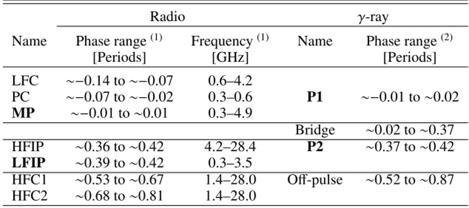
The average pulse profile of the Crab pulsar changes with frequency, showing up to seven different components (Moffett & Hankins 1996; Hankins et al. 2015). In the radio band, below 5 GHz, it consists of the main pulse (MP, at a rota-tion phase from ∼−0.01 to ∼0.01), the low frequency interpulse (LFIP, from ∼0.39 to ∼0.42 in phase), the precursor (PC, from ∼−0.07 to ∼−0.02 in phase, only below 0.6 GHz) and the low frequency component (LFC, from ∼−0.14 to ∼−0.07 in phase, only between 0.6 and 4.2 GHz). At above 5 GHz, the MP van-ishes and an additional interpulse component known as high fre-quency interpulse (HFIP) occurs, which is shifted by about 0.02 with regard to the LFIP and located at ∼0.36 to ∼0.42 in phase. In addition, two components known as high frequency compo-nents (HFC1 at ∼0.53 to ∼0.67 in phase, HFC2 at ∼0.68 to ∼0.81 in phase) appear (Moffett & Hankins 1996;Hankins et al. 2015). The names of all of the components and corresponding phases are summarized in Table1.
Extensive single pulse studies of the Crab pulsar below and above about 5 GHz show even more complex features (Hankins et al. 2016). While MP and LFIP single pulses con-sist of several microsecond long bursts, which can be resolved into single pulses of a duration of nanoseconds with continuous spectra across the observing band, HFIP single pulses consist of one burst of emission of a duration of several microseconds with non-uniform spectra in the form of proportionally spaced emis-sion bands (Hankins et al. 2016). No single pulses of nanosec-ond duration were detected in the case of HFIP single pulses. The observed differences, therefore, suggest similar emission physics for MP and LFIP single pulses and different ones for HFIP single pulses (Hankins et al. 2016).
Single pulses whose flux density is more than ten times higher than the mean are called giant pulses (GPs,Karuppusamy et al. 2010). The pulse widths of radio GPs from the Crab pulsar are in the microseconds to nanoseconds range (Hankins et al. 2003) and their intensity distributions can be described by a power-law (Argyle & Gower 1972). The shortest widths observed so far have been reported to be less than 0.4 ns, resulting in a brightness temperature of about 1041K (Hankins & Eilek 2007). The high brightness temperatures imply a coherent emission mechanism (Hankins et al. 2009). Strong and frequent radio GPs are observed mainly at the phase ranges of MP, LFIP, and HFIP (Jessner et al. 2010;Hankins et al. 2012). Such a complex evolution of the aver-age profile at radio wavelengths has never been observed in any other pulsar so far.
In the γ-ray band, the average pulse profile is smoother and broader than at radio frequencies (Kuiper et al. 2001;Abdo et al. 2010;VERITAS Collaboration 2011;Aleksi´c et al. 2012). Rota-tion phases between −0.01 to ∼0.1 are often called the “P1”, the ones between 0.3 and 0.5 are the “P2”, and the ones between ∼0.1 and 0.3 are known as the “Bridge” (Fierro et al. 1998; Aleksi´c et al. 2014). It is important to note that the MP is included in the P1 range, while LFIP and HFIP are in the P2 range as shown in Table1.
Because of the above mentioned high energy density of GPs in small volumes, a correlation between radio GPs and emission at higher energy bands can be hypothesized (e.g., Eilek & Hankins 2016). One process that could facilitate the required energy release on short spatial and temporal scales is magnetic reconnection in the current sheet outside the light cylinder. In this process, kinetic instabilities break the
frozen-in condition of ideal magnetohydrodynamics (MHD; Contopoulos & Kalapotharakos 2010; Tchekhovskoy et al. 2013), which holds at large1scales and converts magnetic energy into kinetic energy of high energy particles. Both particle-in-cell simulations (Spitkovsky 2006;Cerutti et al. 2012) and analytical descriptions (Contopoulos et al. 1999;Contopoulos 2007) of the pulsar magnetosphere confirmed the existence of current sheets and demonstrated the important role that the magnetic recon-nection mechanism can play (Uzdensky & Spitkovsky 2014). Each stochastically occurring reconnection event would produce radio and high energy emission from synchrotron emission of the energetic particles, for example. Even if a comprehensive theoretical framework does not exist yet, the possibility of finding such a correlation between radio and γ-rays triggered different observations in the γ-ray band.
The Crab pulsar has been also extensively studied in the very-high-energy (VHE) γ-ray range. Imaging Air Cherenkov Telescopes (IACTs) like MAGIC (Major Atmospheric Gamma-ray Imaging Cherenkov telescopes) and VERITAS (Very Ener-getic Radiation Imaging Telescope Array System) revealed that the P2 component is dominant above 50 GeV up to 1.5 TeV, while the P1 component has been measured up to 600 GeV (Aliu et al. 2008; VERITAS Collaboration 2011; Aleksi´c et al. 2012;Ansoldi et al. 2016). The bridge emission is significantly detected only up to ∼150 GeV (Aleksi´c et al. 2014). Any pulsed emission above 25 GeV cannot be explained by the conven-tional polar-cap pulsar models (Ruderman & Sutherland 1975; Daugherty & Harding 1982; Baring 2004) and challenges the slot-gap scenario (Harding et al. 2008), while outer-gap models in which γ-rays are produced by curvature radiation of elec-trons accelerated in the magnetosphere (Hirotani 2008;Tang et al. 2008) are favored.
In the present work, we explore the association between radio GP and VHE (E > 100 GeV) γ-rays. Separate analyses have been conducted in order to search for evidence of com-mon emission between GPs and VHE γ-rays for each of the two γ-ray peaks P1 and P2 (and corresponding radio phases MP and LFIP respectively). From now on, adopting the notation of Aleksi´c et al.(2014), we refer to P1 GPs and P2 GPs to indicate GPs falling inside the VHE γ-rays phase range [−0.01 to 0.02] and [0.37–0.42] respectively: due to the radio frequency consid-ered in the present work (1.4 GHz), this translates to MP GPs and LFIP GPs.
Given that the origin of GPs is not known, it is certainly interesting to search for a correlation between radio GPs and VHE pulsed photons, although there is currently no theoreti-cal approach which describes their correlation. In fact, several searches for multi-wavelength counterparts of radio GPs and optical photons were reported with 7.8σ (Shearer et al. 2003) and 7.2σ (Strader et al. 2013) significance for MP GPs and 1.75σ (Shearer et al. 2003) and 3.5σ (Strader et al. 2013) for LFIP GPs. This result implies the existence of an additional inco-herent emission mechanism associated with radio GPs from the Crab pulsar. Similar studies were carried out in the X-ray band, finding no correlation (Bilous et al. 2012; Mikami et al. 2013, 2014;Aharonian 2018).
Past searches for a correlation between radio GPs and γ-rays from the Crab pulsar provided no positive results either (Argyle et al. 1974; Lundgren et al. 1995; Bilous et al. 2011; Mickaliger et al. 2012). The only other recent study for which data from an IACT was used was carried out by VERITAS (Aliu et al. 2012), who searched for a correlation between radio 1 larger than the kinetic length scales in the plasma.
Table 1. Rotational phase ranges, frequency ranges of occurrence, and nomenclature of average emission components of the Crab pulsar.
Radio γ-ray
Name Phase range(1) Frequency(1) Name Phase range(2)
[Periods] [GHz] [Periods] LFC ∼−0.14 to ∼−0.07 0.6–4.2 PC ∼−0.07 to ∼−0.02 0.3–0.6 P1 ∼−0.01 to ∼0.02 MP ∼−0.01 to ∼0.01 0.3–4.9 Bridge ∼0.02 to ∼0.37 HFIP ∼0.36 to ∼0.42 4.2–28.4 P2 ∼0.37 to ∼0.42 LFIP ∼0.39 to ∼0.42 0.3–3.5 HFC1 ∼0.53 to ∼0.67 1.4–28.0 Off-pulse ∼0.52 to ∼0.87 HFC2 ∼0.68 to ∼0.81 1.4–28.0
Notes.(1)Radio phase ranges and frequency values are taken fromHankins et al.(2015).(2)γ-ray phase ranges are taken fromAleksi´c et al.(2014).
GPs at 8.9 GHz and VHE γ-rays with energies higher than 150 GeV. With a total overlap of 11.6 h, they reported upper lim-its of five to ten times the average Crab pulsar VHE flux on the flux measured simultaneously with P2 GPs and of two to three times the average VHE flux on time scales of about eight sec-onds around P2 GPs. The present study focuses on the search for a correlation between radio GPs from the Crab pulsar and its VHE γ-ray emission. The differences with respect to the study carried out by the VERITAS Collaboration inAliu et al.(2012) are the following: firstly, the corresponding radio data presented here were taken at a center frequency of about 1.4 GHz, whereas radio observations described in Aliu et al. (2012) were carried out at 8.9 GHz. Based on the results by Hankins et al.(2016) we are addressing a different population of radio GPs. Secondly, the γ-ray observations reported here were carried out at ener-gies above 60 GeV, where the P1 emission is pronounced, while inAliu et al. (2012) the energy threshold was above 150 GeV, where the P1 emission is much fainter (Aleksi´c et al. 2012). The lower energy threshold of MAGIC (Ethr ∼ 60 GeV) in
compar-ison with the energy threshold of VERITAS (Ethr ∼ 150 GeV)
allows a more comprehensive analysis of the correlation between VHE γ-rays and the P1 GPs. Thirdly, the amount of simultane-ous observations between VHE γ-rays and radio is larger in the present study (16 h vs. 11.6 h), corresponding to the currently largest sample of simultaneous VHE γ-rays and radio GP data taken with an IACT.
The paper is organized as follows: the observations and data analysis are described in Sect.2. The construction of the Monte Carlo (MC) simulations is described together with the correla-tion study in Sect. 3. The results are discussed in Sect.4 and a summary can be found in Sect.5. The AppendixAcarries a detailed explanation of the MC simulations developed specifi-cally for this study.
2. Observations and data reduction
2.1. Radio observations
The radio observations were carried out with the Effelsberg radio telescope and the Westerbork Synthesis Radio Telescope (WSRT) at a frequency of about 1.4 GHz. The two facilities scheduled complementary observations in order to exclude over-laps in the recorded data sample. Observations of the Crab pulsar with the Effelsberg radio telescope were carried out in baseband mode with the P217 mm and P200 mm prime focus receivers and the PSRIX pulsar backend (Lazarus et al. 2016). The Crab
pulsar observations taken with the WSRT were carried out with 13 out of 14 available antennas, their Multi-frequency Front End Receivers (MFFEs,Casse et al. 1982;Tan et al. 1991), and the PuMa II pulsar backend (Karuppusamy et al. 2008).
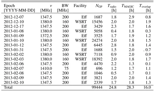
All radio data sets were coherently dedispersed (Hankins & Rickett 1975) during an off-line reduction pro-cess. For this part of the reduction the digital library DSPSR (van Straten & Bailes 2011) was used. After the dedispersion procedure, the resulting data sets were phase folded with ephemeris files obtained from the Jodrell Bank Observatory (Lyne et al. 1993). To ensure absolute alignment between the radio and γ-rays pulses, an ephemeris which covered the observing days was created and used instead of the monthly released one. To extract the brightest single pulses, an additional data selection, based on the standard deviation of the signal in the OFF-pulse radio emission regions, was introduced in the dedispersed data sets. With this technique, a total number of 99 444 GPs was extracted from the radio data. A summary of all the radio observations performed for this study is given in Table2 and a corresponding phase diagram of an observation taken with the Effelsberg telescope and the WSRT is shown in Fig.1. 2.2.γ-ray observations
VHE γ-ray observations were carried out with the MAGIC tele-scopes between December 2012 and February 2013 (simultane-ously with observations either with the Effelsberg radio tele-scope, or the WSRT). They were taken at zenith angles of less than 30◦ to achieve the lowest possible energy thresh-old, and with both telescopes in Wobble observation mode (Fomin et al. 1994). The reduction of the resulting data was carried out according to the standard analysis pipeline using the MAGIC Analysis and Reconstruction Software (MARS, Zanin et al. 2013).
To efficiently suppress the hadronic background without losing a large fraction of air showers induced by VHE pho-tons from the Crab pulsar, energy dependent cuts in Hadroness (a test statistic for discrimination between a γ-ray or a hadron induced shower) and θ2 (the squared angular distance between
the expected source position and the reconstructed one) param-eters were performed (details inAleksi´c et al. 2016). They were optimized on an independent data sample of 46 h of observa-tions, taken at zenith angles of less than 30◦, same as the main data set used in the present work. For an energy range span-ning from 5 GeV to 50 TeV, 30 logarithmic energy bins were defined. In each energy bin the Hadroness and θ2 parameters
Table 2. Summary of radio and VHE γ-ray observations.
Epoch ν BW Facility NGP Tradio TMAGIC Toverlap
[YYYY-MM-DD] [MHz] [MHz] [h] [h] [h] 2012-12-07 1347.5 200 Eff 1687 1.8 2.9 0.8 2012-12-10 1380.0 160 WSRT 15456 2.0 2.0 1.9 2012-12-17 1347.5 200 Eff 3429 2.3 1.7 1.6 2013-01-08 1380.0 160 WSRT 5058 0.4 1.8 0.3 2013-01-09 1372.5 200 Eff 3525 1.7 1.9 1.2 2013-01-10 1380.0 160 WSRT 24274 2.0 1.8 1.5 2013-01-12 1347.5 200 Eff 6445 2.8 1.8 1.4 2013-01-31 1347.5 200 Eff 1688 1.5 2.0 . 0.7 2013-02-02 1380.0 160 WSRT 7118 0.9 2.0 0.9 2013-02-03 1380.0 160 WSRT 18392 2.0 1.8 1.7 2013-02-06 1347.5 200 Eff 4470 2.2 1.3 0.1 2013-02-07 1410.0 75 Eff 696 1.2 1.7 1.1 2013-02-08 1347.5 200 Eff 1046 0.5 1.7 0.1 2013-02-09 1347.5 200 Eff 3821 2.0 2.0 1.4 2013-02-10 1347.5 200 Eff 2339 1.7 1.8 1.3 Total 99444 24.8 28.3 16.0
Notes. The value ν stands for the center frequency, BW for the bandwidth, NGP for the number of extracted GPs, Tradio and TMAGICindicate the duration of the radio and the corresponding VHE γ-rays observation respectively. The acronym Eff stands for Effelsberg radio telescope while WSRT for Westerbork Synthesis Radio Telescope.
0.0 0.5 1.0 1.5 2.0 0.0 0.2 0.4 0.6 0.8 1.0 1.2 1.4 1.6 1.8 2.0 Flux [A.U .] Phase P1 0.0 0.5 1.0 1.5 2.0 0.96 0.98 1.00 1.02 1.04 P2 0.0 0.5 1.0 1.5 2.0 0.36 0.38 0.40 0.42 0.44
Fig. 1. Phase diagram resulting from one Effelsberg observation (2017-12-07, red solid curve) and one WSRT observation (2017-12-10, green dashed curve). MP is visible near phase 0.0 and 1.0 whereas LFIP near phases 0.4 and 1.4. The blue dotted curve represents the sum of both observations.
were optimized to maximize the significance of the pulsed γ-ray signal, taking the continuous emission from the Crab Nebula as described inAleksi´c et al.(2012) into account.
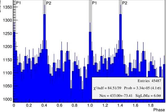
After optimizing the cuts in each energy bin separately we picked the bins in the energy range from 42.9 to 367.8 GeV that correspond to the energy range in Aleksi´c et al. (2012). The 16 h of VHE γ-ray data taken simultaneously with radio observations led to a detection of the pulsar clearly above the background of the Crab Nebula (with 6.0σ significance) in that range, as shown in Fig. 2. For the barycentering of the VHE γ-ray data the TEMPO2 pulsar timing software (Hobbs et al. 2006) and the same ephemeris files were used as for the radio data (Lyne et al. 1993). The folded light curve obtained after the barycentering process and the selection cuts are shown in Fig.2: the gray shadowed areas are the results from a previous MAGIC phase resolved analysis of the Crab pulsar (Aleksi´c et al. 2012). The overlap with the present data (blue filled area) shows the compatibility between the two analyses, even if the energy
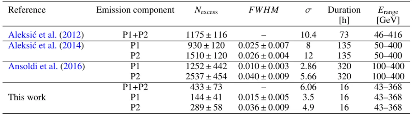
ranges for the two results are slightly different (our results are shown here for the energy range from 43 to 368 GeV while results from Aleksi´c et al. 2012 were obtained in the energy range from 50 to 400 GeV). To further quantify the compati-bility with previous MAGIC results, we report in Table 3 the number of excess events, significance and the full width at half maximum (FWHM) of a Gaussian fit to the peaks of P1 and P2 respectively, from the work ofAleksi´c et al. (2012, 2014), Ansoldi et al.(2016) and compare those with our results.
3. Correlation study
3.1. Approach
Due to the lack of statistical methods for the correlation analy-sis of independent event lists2, but also for comparability with 2 A discussion of that problem can be found in Edelson & Krolik (1988).
Phase 0 0.2 0.4 0.6 0.8 1.0 1.2 1.4 1.6 1.8 Events 1000 1050 1100 1150 1200 1250 1300 1350 Entries 45487 ) σ /ndf = 84.51/39 Prob = 3.34e-05 (4.1 2 χ σ Nex = 433.00+-73.41 SigLiMa = 6.0 P1 P2 P1 P2
Fig. 2. Phase diagram resulting from the MAGIC data after the barycenter-ing process and the cut selection, in the energy range 43–368 GeV. The resulting significance is 6σ. The gray areas corre-spond with the pulsed emission regions as determined by Aleksi´c et al. (2012) for the energy range 50–400 GeV. P1 is visible around phase values of 0 and 1, whereas P2 is located around 0.4 and 1.4.
results from previous studies with IACT data, we adopted the approach described inAliu et al. (2012). The number of coin-cidences between VHE γ-rays and GPs was counted inside a given search window (SW, see Fig. 3). SWs were defined in terms of fractions or multiples of one rotational period of the Crab pulsar, namely: 1/9, 1/3, 1, 3, 9, 27, 81, 243, 729, 2187. With the aim of reducing the background emission from the Crab Nebula in our analysis, and to conduct dedicated studies on P1 and P2 respectively, we extended the approach of Aliu et al. (2012) by adopting SWs smaller than one rotational period (1/9 and 1/3). Exploring different SWs allowed us to change the trade-off between statistical and systematic uncertainties. More-over, the SWs smaller than one that we consider in the present work only contain one of the pulsed emission components, either P1 or P2, depending at which phase range the radio GPs are located. Hence, SWs smaller than one rotation period of the Crab pulsar describe here the increase of VHE photons centered on radio GPs from only one of the regular emission components instead of both, allowing us to perform two separate analyses focused on P1 GPs and P2 GPs. As explained in Sect. 1, the indication of different emission mechanisms of GPs in P1 and P2 makes the separated analysis an important tool to deeply inves-tigate the possible coincidences between GPs at various phase ranges at different energies.
Since the emission mechanism of radio GPs is unknown, a delay in the generation of radio GPs and VHE photons cannot be excluded. Therefore the search windows were constructed for three different orientations in time: before, centered on, and after a radio GP (see Fig.3). This way possible time delays between the generation of radio GPs and VHE γ-rays were included in the search procedure. The described approach results in a total of 30 correlation searches.
3.2. Monte Carlo simulations 3.2.1. Radio simulations
Two statistical properties of the radio data were reproduced in the MC simulations: the average phase profile which we modeled by two Gaussians and the interarrival time between
subsequent GPs. We modeled the interarrival times directly from the observed separations.
The interval between successive GPs was calculated and stored in a list. The list of interarrival times derived from obser-vations was used instead of an analytic exponential distribution for two reasons: (1) There were non-trivial deviations from the exponential distribution due to the phase bound occurrence of radio GPs; (2) There were deviations at large time separations (more than 50 rotation periods) due to the fact that the observa-tions at both telescopes were interrupted by weather, data write-out and other technical constraints.
Due to time gaps within the radio data sets (introduced dur-ing data recorddur-ing to produce data chunks which were shorter in time and thus easier to reduce off-line), all interarrival times longer than 30 s were excluded from the simulation. All inter-arrivals shorter than this threshold were stored in a list. In the MC simulation a random interarrival time was fetched from the above-described list instead of drawing from an analytic expo-nential distribution. The parameters of the average profile were obtained by fitting Gaussian distributions to the P1 and P2 com-ponents in the radio data. To increase the signal-to-noise-ratio, the fit was performed on all the radio data collected during this campaign, with the exception of the Effelsberg data sets from 2013-01-09 and 2013-02-07 since both were taken at different center frequencies (see Table 2). A more detailed explanation can be found inLewandowska(2015).
3.2.2.γ-ray simulations
In order to asses the significance level of the correlation, we pro-duced correlation-free γ-ray data and searched for a correlation with the real radio data. The synthetic data had to reflect all the statistical properties of the real data. We produced such a data set in the following way3:
1. The rate of events (before selection by Hadroness or θ2
parameters) was converted into a cumulative distribution func-tion (CDF) with bin widths of one second.
Table 3. Comparison of the current data set with previous MAGIC observations of the pulsed emission from the Crab Nebula.
Reference Emission component Nexcess FW H M σ Duration Erange
[h] [GeV] Aleksi´c et al.(2012) P1+P2 1175 ± 116 – 10.4 73 46–416 Aleksi´c et al.(2014) P1 930 ± 120 0.025 ± 0.007 8 135 50–400 P2 1510 ± 120 0.026 ± 0.004 12 135 50–400 Ansoldi et al.(2016) P1 1252 ± 442 0.010 ± 0.003 2.86 320 100–400 P2 2537 ± 454 0.040 ± 0.009 5.66 320 100–400 P1+P2 433 ± 73 – 6.06 16 43–368 This work P1 144 ± 41 0.015 ± 0.005 3.5 16 43–368 P2 289 ± 58 0.036 ± 0.009 4.9 16 43–368
2. A uniform random number was drawn and the first bin in the CDF was located where the fraction of events exceeds that random number.
3. A second uniform random number was drawn in order to determine a time stamp in the one second interval covered by the bin.
4. The time stamp obtained in step 3 does not yet reflect the fact that the VHE γ-ray data contains the pulsations from the Crab pulsar. Therefore, the time stamp was slightly modified in the fol-lowing way: the event stayed within the same pulsar period, but the phase inside the rotation was drawn from a model containing a uniform background and two Gaussian peaks. This model was obtained by fitting the observed pulsed profile (after Hadroness and θ2 cuts). The adjusted phase was then converted back into a time value using the Taylor expansion formula (Eq. (8.4) in Lorimer & Kramer 2012).
5. The steps 2, 3, and 4 were repeated M times. For each MC data set, M was drawn randomly from a Poisson distribution with a mean of Nproc, where Nprocis the total number of events
after Hadroness and θ2 cuts. This way, one can get a synthetic
uncorrelated VHE γ-ray data set with M events.
To calculate confidence intervals with sufficiently low sta-tistical error, 200 different synthetic VHE γ-ray data sets were produced by repeating the above procedure. As shown below in Sect. 3.3, we did not find a statistically significant correlation. Therefore we calculated and report upper limits to the degree of correlation. For this purpose we defined a correlation parame-ter κ, which is the fraction of γ-ray events arriving simultane-ously to an observed GP. Using this parameter we also generated synthetic correlated γ-ray data sets with different values of the parameter κ. At first we generated a uncorrelated γ-ray signal using the described procedure, but the arrival times of κ · Npulse
events were replaced by randomly picked arrival times of radio GPs, Npulse being the number of detected pulsed events in the
real VHE γ-ray data. 3.3. Results
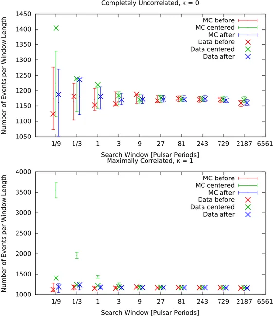
The number of coincidence events in the observational data for different SWs are shown in Fig. 4, together with the uncorre-lated simulation results (top) and the perfectly correuncorre-lated (κ= 1) simulation results (bottom). Error bars for simulation results are obtained as a 1σ fluctuation among 200 data sets (see Sect.3.2). As can be deduced from the top panel of Fig.4, the observed enhancement of VHE γ-rays becomes higher for shorter search windows centered on a GP, though the bottom panel shows the correlation is well below 100%. Therefore, only the number of VHE photons in a search window centered on a radio GP for a window length of 1/9, 1/3, 1 and 3 Crab pulsar rotation periods
t
tGP
before centered after
Fig. 3.Construction of search windows around a radio GP. The cen-tral window is symmetric around the arrival time of a radio GP. The advanced and delayed windows have the same length and are adjacent in time to the centered window. This construction arranges the search windows in a hierarchy where all three search windows of one length together form the centered search window of the next larger duration.
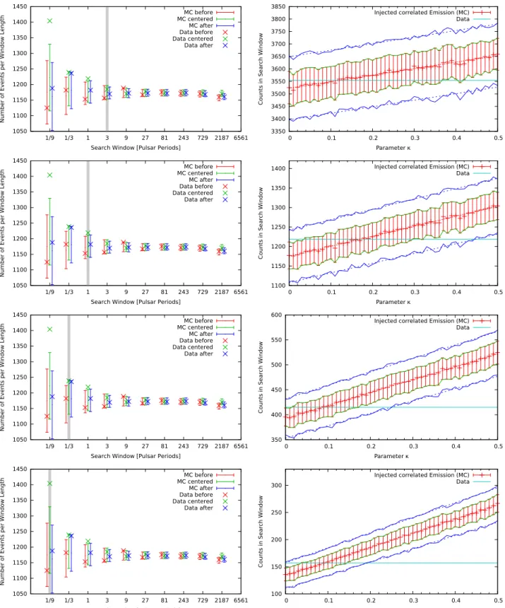
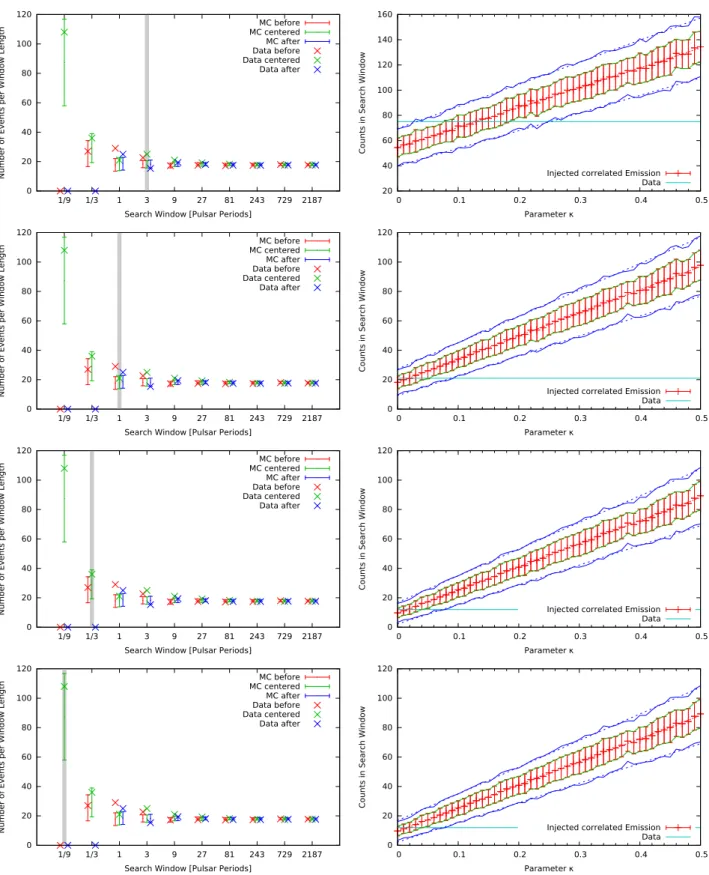
are examined in the forthcoming part of the analysis. To deter-mine the enhancement quantitatively, MC simulations with dif-ferent κ values are compared with the corresponding data point. The results are shown in the right hand plots of Fig.5.
The cyan line represents the data point from the respective search window. The red ticks correspond to the average values of the VHE γ-ray MC simulations for different values of κ. The 1σ range around the average values is indicated by the vertical red bars as well as the green lines. The blue lines stand for the 1.96σ range. Since a linear scaling of both the average and the upper and lower limits are expected, the plot also contains fitted linear trend lines as dashed curves. To determine the best estimated value of κ which reflects the enhancement of VHE γ-rays seen in the data, we calculate the intersection of the horizontal cyan data line with the linear trend lines4. This procedure is carried out for all four search window lengths. The corresponding results are given in the upper four rows of Table4. The most significant deviation of κbest
is seen at a search window of 1/9 of the rotation period, which is in accordance with Fig.4. Since none of the κbestis significantly
larger than 0, 95% level upper limits on κ are also calculated on each window size, as the intersection between the cyan and blue lines in the figure. They are shown in the column of “CI95%” in
Table4.
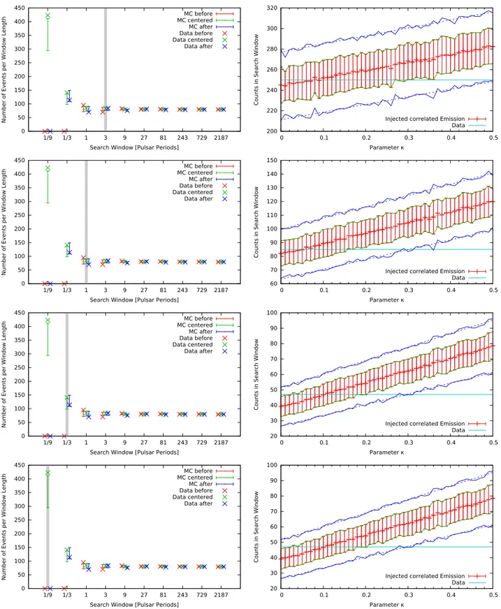
In order to differentiate between P1 and P2 GPs (which cor-respond in this particular analysis to MP and LFIP as discussed in Sect.1), we carry out the same analysis with radio GPs only within the phase ranges between −0.02 and 0.02 (centered on MP radio phase) and between 0.37 and 0.42 (centered on LFIP radio phase, see Table1). The corresponding results are shown in Figs.6and7and are summarized in Table4.
4 In one case (SW= 3) this required extrapolation to κ > 0.5, beyond the range for which MCMC simulations were performed.
1050 1100 1150 1200 1250 1300 1350 1400 1450 1/9 1/3 1 3 9 27 81 243 729 2187 6561 Number of E vents per W indo w Len gth
Search Window [Pulsar Periods] Completely Uncorrelated, κ = 0 MC before MC centered MC after Data before Data centered Data after 1000 1500 2000 2500 3000 3500 4000 1/9 1/3 1 3 9 27 81 243 729 2187 6561 Number of E vents per W indo w Len gth
Search Window [Pulsar Periods] Maximally Correlated, κ = 1 MC before MC centered MC after Data before Data centered Data after
Fig. 4.Enhancement of VHE photons around occurring radio GPs resulting out of data sets (marked with crosses) and VHE γ-ray MC simulations (indicated by bars). Upper plot: results for a perfectly uncorrelated VHE γ-ray signal in the MC simulations (κ = 0), while lower plot: flux enhancement results for an injected VHE γ-ray signal which is perfectly correlated with GPs resulting from the radio data in a centered search window (κ= 1). The latter plot shows more clearly an increase of the number of VHE γ-rays centered on radio GPs for shorter search windows resulting from the data sets, indicating that the correlation is located at κ < 1.
4. Discussion
The present results do not show a statistically significant corre-lation between radio GPs and VHE γ-rays from the Crab pul-sar. No correlation was found also in several studies carried out in the past, including the work of Argyle et al. (1974), Lundgren et al. (1995), Bilous et al. (2011), Mickaliger et al. (2012), and Aliu et al.(2012). A correlation with optical pho-tons was found byShearer et al.(2003), as a 3% higher average intensity over many periods with GPs observed. In order to com-pare this study with previous ones, it is useful to convert κ to the factor of flux enhancement during GPs. It can approximately be done as follows. Upper limits in number of γ-rays accompanied with a radio GP (NUL) are
NUL= κUL· Nγ, (1)
where Nγ is the number of observed pulsed γ-rays which is 443.0 ± 73.4 as shown in Fig.2. Total observation time “around
GPs” TGP can be computed from the number of obtained GPs
NGPand the size of the search window TSWas
TGP= NGP· TSW= NGP· PCrab· fSW, (2)
where fSWis the search window in fraction of the rotation period,
such as 1/9, 1/3, 1 and 3 for this study. Since NGP is 99 444 as
shown in Table2, TGP' 0.93 · fSWh.
NUL/TGP should be compared with Nγ/Ttotal, where Ttotalis
the total observation time which is 16 h. Then, the upper limit in the flux enhancement FULis written as
FUL= (NUL/TGP)/(Nγ/Ttotal) (3)
=(κ · Nγ)/(NGP· PCrab· fSW)
Nγ/Ttotal
(4)
= 17.3 · κ/ fSW (5)
Therefore, the upper limit in κ of 0.45 for fSW = 1 (see
1050 1100 1150 1200 1250 1300 1350 1400 1450 1/9 1/3 1 3 9 27 81 243 729 2187 6561 Number of E vents per W indo w Len gth
Search Window [Pulsar Periods] MC before MC centered MC after Data before Data centered Data after 3350 3400 3450 3500 3550 3600 3650 3700 3750 3800 3850 0 0.1 0.2 0.3 0.4 0.5 Coun ts in Sea rch W indow Parameter κ
Injected correlated Emission (MC) Data 1050 1100 1150 1200 1250 1300 1350 1400 1450 1/9 1/3 1 3 9 27 81 243 729 2187 6561 Number of E vents per W indo w Len gth
Search Window [Pulsar Periods] MC before MC centered MC after Data before Data centered Data after 1100 1150 1200 1250 1300 1350 1400 0 0.1 0.2 0.3 0.4 0.5 Coun ts in Sea rch W indow Parameter κ
Injected correlated Emission (MC) Data 1050 1100 1150 1200 1250 1300 1350 1400 1450 1/9 1/3 1 3 9 27 81 243 729 2187 6561 Number of E vents per W indo w Len gth
Search Window [Pulsar Periods] MC before MC centered MC after Data before Data centered Data after 350 400 450 500 550 600 0 0.1 0.2 0.3 0.4 0.5 Coun ts in Sea rch W indow Parameter κ
Injected correlated Emission (MC) Data 1050 1100 1150 1200 1250 1300 1350 1400 1450 1/9 1/3 1 3 9 27 81 243 729 2187 6561 Number of E vents per W indo w Len gth
Search Window [Pulsar Periods] MC before MC centered MC after Data before Data centered Data after 100 150 200 250 300 0 0.1 0.2 0.3 0.4 0.5 Coun ts in Sea rch W indow Parameter κ
Injected correlated Emission (MC) Data
Fig. 5.From top to bottom: search windows of 3, 1, 1/3 and 1/9 Crab pulsar rotation periods length. Left: enhancements of VHE γ-rays before,
centered on and after a radio GP. The gray bar indicates the search window for which the κ dependence is studied in the respective right hand plot. Right: horizontal cyan line indicates the number of VHE γ-rays in the search window centered on GPs (the corresponding value from the observed data is indicated by a cross in the left hand plot. The normalization of the y-axis between the two columns is different). The plot also contains the results from 50 different sets of γ-ray MC simulations, using different values of κ. The average of each set is indicated by a red tick. The 1σ range is indicated by the green lines, the 1.96σ range (corresponding to a rejection of the null hypothesis on a p= 0.05 confidence level) is indicated by the blue lines.
0.19 for SW= 1/9 translates to 2900%. This calculation shows that the sensitivity at γ-ray energies and telescope time avail-able for this study are not sufficient to detect a statistically
significant correlation, or place an upper constraint compara-ble to the correlation observed in the optical regime. The corre-sponding expressions in Eq. (5) for the phase resolved analysis
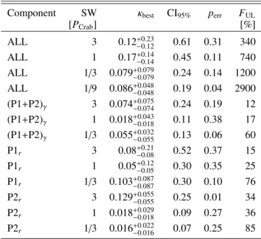
Table 4. Results of the correlation study between radio GPs and γ-rays that appear to be correlated with radio GPs (resulting from the intersec-tion values between linear fits of γ-ray MC simulaintersec-tions and data points in the right hand figures of Figs.6and7).
Component SW κbest CI95% perr FUL
[PCrab] [%] ALL 3 0.12+0.23−0.12 0.61 0.31 340 ALL 1 0.17+0.14−0.14 0.45 0.11 740 ALL 1/3 0.079+0.079−0.079 0.24 0.14 1200 ALL 1/9 0.086+0.048−0.048 0.19 0.04 2900 (P1+P2)γ 3 0.074+0.075−0.074 0.24 0.19 12 (P1+P2)γ 1 0.018+0.043−0.018 0.11 0.38 17 (P1+P2)γ 1/3 0.055+0.032−0.055 0.13 0.06 60 P1r 3 0.08+0.21−0.08 0.52 0.37 15 P1r 1 0.05+0.12−0.05 0.30 0.35 25 P1r 1/3 0.103+0.087−0.087 0.30 0.10 76 P2r 3 0.129+0.055−0.055 0.25 0.01 34 P2r 1 0.018+0.029−0.018 0.09 0.27 36 P2r 1/3 0.016+0.022−0.016 0.07 0.25 85
Notes. The first column indicates the used data sample without phase cuts (marked “ALL”), only P1 and P2 in the VHE γ-ray data+ MCs (marked with a γ) and P1, P2 based on Gaussian fits in the radio data (marked with an “r”). Their indices reflect whether the phase cuts are based on the radio, or γ-ray data. The acronym SW is standing for search window length, PCrab is the rotation period of the Crab pulsar, κbestis the intersection value, CI95%is the upper value of the correspond-ing 95% confidence interval, perrthe probability to obtain the observed number of events based on the mean and standard deviation of the MC simulations and FULthe upper limit of the flux normalized to the pulsed VHE flux of the Crab pulsar.
are FUL,P1 = 0.848 ∗ κ/ f and FUL,P2 = 4.04 ∗ κ/ f , accounting
for the number of GPs (82 055 and 17 041, respectively) and the shortening of Ttotaldue to the phase cuts.
The only existing theoretical prediction for a correlation at frequencies higher than 5 GHz is given by Lyutikov (2007). However, this model is applicable to radio GPs at the phase ranges of P2 above 5 GHz, which does not cover the fre-quency range of the observations presented in this work, mak-ing the model not applicable to our observations. The studies by Bilous et al.(2011) andAliu et al.(2012) addressed radio GPs above 5 GHz, and reported 95% confidence level upper limits on the enhanced flux of five to ten times higher the flux measured by VERITAS. The higher energy threshold of VERITAS combined with the steep power-law spectrum of the Crab pulsar may have limited the sensitivity of the study. The correlation study carried out byMickaliger et al.(2012) at 300 MHz and 1.2 GHz did not result in any statistically significant findings in spite of extended searches for coincidences between radio GPs and GeV γ-rays. In the latter case data taken by the Large Area Telescope (LAT) on board the Fermi satellite (Abdo et al. 2009) were used which, in comparison with the present work, provided data with a lower background. The data set was spanning over 15 months but the smaller collection area of the space-borne detector could be a limiting factor regarding the number of detected events which might be the reason for not detecting any correlation. The Hit-omi X-ray satellite also searched for a correlation between radio
GPs and soft X-rays. Aharonian(2018) report upper limits of 22%–80% of the peak flux at a range of 2–300 keV.
A recent review on the radio emission physics of the Crab pulsar given byEilek & Hankins(2016) suggests that the observed radio and high energy emission might have origin in the same spatial regions within the magnetosphere, due to the fact that both, main radio and high energy emission components, appear approximately at the same phase ranges. However, a sat-isfactory theoretical approach still needs to be found. The variety of instabilities in the radio emission of the Crab pulsar (includ-ing GPs) leads to the assumption that the radio emission sites are dynamic and unstable (Eilek & Hankins 2016). The connec-tion between these regions and the high energy emission is still an open question. Since the Crab pulsar has been an object of regular monitoring campaigns at radio (Lyne et al. 1993) as well as at VHE γ-ray wavelengths (Meyer et al. 2010), we suggest a coordination of the respective observations. Simultaneous obser-vations at both energy ranges can lead to a further examination of the obtained results, especially below and above 5 GHz by including radio GPs from the Crab pulsar at frequencies before and after the described transition.
5. Summary
In this work a correlation study between radio GPs and γ-rays above 60 GeV from the Crab pulsar is presented. The data used for this study were taken with the Effelsberg radio telescope (at 1347.5 MHz and 1410 MHz), the WSRT (at 1380.0 MHz) and the MAGIC telescopes (Figs.1and2). The total overlap between the radio and γ-ray observations (excluding all gaps which are longer than 30 s) results in 16 h (see Table2). The approach for our correlation search is based on the idea described inAliu et al. (2012), consisting of the construction of search windows around the arrival time of each radio GP resulting from the radio data (see Fig.3). We compare the amount of VHE γ-rays around a radio GP resulting from the observational data and MC simula-tions which are based on the timing characteristics of the data. To estimate the degree of correlation, we inject a variable level of a signal which is perfectly correlated with radio GPs into the sim-ulations. With this approach we determine the fraction of VHE photons which appear to be correlated with radio GPs (indicated by component “ALL” and denoted as κbestin Table4).
Based on the described study, we conclude the following: – No statistically significant correlation between VHE pulsed
photons and radio GPs at 1.4 GHz was found for search win-dow sizes of 1/9, 1/3, 1, and 3 times the rotation period. – The most stringent upper limit in the correlation degree
was obtained for the search window of 1/9 of the rotational period, and not more than 19% of the γ-rays are accom-panied by GPs. This corresponds to an upper limit on the increase in pulsed flux of no more than 2900% at 95% con-fidence level.
– GPs in MP and LFIP are separately analyzed, and the corre-sponding upper limits are presented in Table4. Converting the correlation to a flux enhancement relative to the pulsed flux, we find upper limits between 15% (P1 phase cut, search window of 3 PCrab) and 85% (P2 phase cut, search window
of 1/3 PCrab). The phase cuts do allow to place more stringent
upper limits, but no statistically significant correlation could be found.
Future observations with a larger overlap or higher sensitivity, as hopefully provided by the Cherenkov Telescope Array (CTA, Acharya et al. 2013;CTA Consortium 2019), will help to pro-vide further constraints in the still open question of a correlation
0 50 100 150 200 250 300 350 400 450 1/9 1/3 1 3 9 27 81 243 729 2187 Number of E vents per W indo w Len gth
Search Window [Pulsar Periods] MC before MC centered MC after Data before Data centered Data after 200 220 240 260 280 300 320 0 0.1 0.2 0.3 0.4 0.5 Coun ts in Sea rch W ind ow Parameter κ
Injected correlated Emission Data 0 50 100 150 200 250 300 350 400 450 1/9 1/3 1 3 9 27 81 243 729 2187 Number of E vents per W indo w Len gth
Search Window [Pulsar Periods] MC before MC centered MC after Data before Data centered Data after 60 70 80 90 100 110 120 130 140 150 0 0.1 0.2 0.3 0.4 0.5 Coun ts in Sea rch W ind ow Parameter κ
Injected correlated Emission Data 0 50 100 150 200 250 300 350 400 450 1/9 1/3 1 3 9 27 81 243 729 2187 Number of E vents per W indo w Len gth
Search Window [Pulsar Periods] MC before MC centered MC after Data before Data centered Data after 20 30 40 50 60 70 80 90 100 0 0.1 0.2 0.3 0.4 0.5 Coun ts in Sea rch W ind ow Parameter κ
Injected correlated Emission Data
Fig. 6.Results as described in Fig.5for the P1 emission component (MP radio phase). The MC error bars in the left hand part of this figure were computed for κ= 0 and not for the best fit κ value.
between radio GPs and the VHE γ-ray emission from the Crab pulsar.
Acknowledgements. NL would like to thank Axel Jessner (MPIfR), Jean Eilek (NRAO), Maura McLaughlin (WVU), Ryan Lynch (GBO) and Vlad Kondratiev (ASTRON) for numerous helpful comments which improved the quality of
the paper. We acknowledge Marina Manganaro (Croatian MAGIC Consortium) for her continuous help in preparing the manuscript. We would like to thank the anonymous referee for numerous comments which helped us to improve the quality of the manuscript. NL would also like to thank Ramesh Karup-pusamy (MPIfR), Alex Kraus (MPIfR), Ralf Kisky (MPIfR), Jörg Barthel (MPIfR) and Thomas Wedel (MPIfR) for constant support during the obser-vations with the Effelsberg radio telescope. NL gratefully acknowledges the
0 20 40 60 80 100 120 1/9 1/3 1 3 9 27 81 243 729 2187 Number of E vents per W indo w Len gth
Search Window [Pulsar Periods] MC before MC centered MC after Data before Data centered Data after 20 40 60 80 100 120 140 160 0 0.1 0.2 0.3 0.4 0.5 Coun ts in Sea rch W ind ow Parameter κ
Injected correlated Emission Data 0 20 40 60 80 100 120 1/9 1/3 1 3 9 27 81 243 729 2187 Number of E vents per W indo w Len gth
Search Window [Pulsar Periods] MC before MC centered MC after Data before Data centered Data after 0 20 40 60 80 100 120 0 0.1 0.2 0.3 0.4 0.5 Coun ts in Sea rch W ind ow Parameter κ
Injected correlated Emission Data
Fig. 7.Results as described in Figs.5and6for the P2 emission component (LFIP radio phase).
support of this study by the ASTRON/JIVE Helena Kluyver female visitor program. This study is partly based on observations with the 100-m telescope of the MPIfR (Max-Planck-Institut für Radioastronomie) at Effelsberg. Another part of this study was carried out with data taken with the Westerbork Syn-thesis Radio Telescope (WSRT). The Westerbork SynSyn-thesis Radio Telescope is operated by the ASTRON (Netherlands Institute for Radio Astronomy) with support from the Netherlands Foundation for Scientific Research (NWO). We would like to thank the Instituto de Astrofísica de Canarias for the excel-lent working conditions at the Observatorio del Roque de los Muchachos in
La Palma. The financial support of the German BMBF and MPG, the Italian INFN and INAF, the Swiss National Fund SNF, the ERDF under the Spanish MINECO (69818-P, FPA2012-36668, 68378-P, FPA2015-69210-C6-2-R, FPA2015-69210-C6-4-R, FPA2015-69210-C6-6-R, AYA2015-71042-P, AYA2016-76012-C3-1-P, ESP2015-71662-C2-2-P, CSD2009-00064), and the Japanese JSPS and MEXT is gratefully acknowledged. This work was also supported by the Spanish Centro de Excelencia “Severo Ochoa” SEV-2012-0234 and SEV-2015-0548, and Unidad de Excelencia “María de Maeztu” MDM-2014-0369, by the Croatian Science Foundation (HrZZ) Project 09/176 and the
University of Rijeka Project 13.12.1.3.02, by the DFG Collaborative Research Centers SFB823/C4 and SFB876/C3, the Polish National Research Centre grant UMO-2016/22/M/ST9/00382 and by the Brazilian MCTIC, CNPq and FAPERJ.
References
Abdo, A. A., Ackermann, M., Ajello, M., et al. 2009,ApJS, 183, 46 Abdo, A. A., Ackermann, M., Ajello, M., et al. 2010,ApJ, 708, 1254 Acharya, B. S., Actis, M., Aghajani, T., et al. 2013,Astropart. Phys., 43, 3 Aleksi´c, J., Alvarez, E. A., Antonelli, L. A., et al. 2012,A&A, 540, A69 Aleksi´c, J., Ansoldi, S., Antonelli, L. A., et al. 2014,A&A, 565, L12 Aleksi´c, J., Ansoldi, S., Antonelli, L. A., et al. 2016,Astropart. Phys., 72, 76 Aliu, E., Anderhub, H., Antonelli, L. A., et al. 2008,Science, 322, 1221 Aliu, E., Archambault, S., Arlen, T., et al. 2012,ApJ, 760, 136 Ansoldi, S., Antonelli, L. A., Antoranz, P., et al. 2016,A&A, 585, A133 Argyle, E., & Gower, J. F. R. 1972,ApJ, 175, L89
Argyle, E., Baird, G., Grindlay, J., Helmken, H., & Omongain, E. 1974,Nuovo Cimento B Serie, 24, 153
Baring, M. G. 2004,AdSpR, 33, 552
Bilous, A. V., Kondratiev, V. I., McLaughlin, M. A., et al. 2011,ApJ, 728, 110 Bilous, A. V., McLaughlin, M. A., Kondratiev, V. I., & Ransom, S. M. 2012,ApJ,
749, 24
Casse, J. L., Woestenburg, E. E. M., & Visser, J. J. 1982,IEEE Trans. Microwave Theory Tech., 30, 201
Cerutti, B., Werner, G. R., Uzdensky, D. A., & Begelman, M. C. 2012, in American Institute of Physics Conference Series, eds. F. A. Aharonian, W. Hofmann, & F. M. Rieger, 1505, 631
Contopoulos, I. 2007,A&A, 472, 219
Contopoulos, I., & Kalapotharakos, C. 2010, in 9th International Conference of the Hellenic Astronomical Society, eds. K. Tsinganos, D. Hatzidimitriou, & T. Matsakos,ASP Conf. Ser., 424, 128
Contopoulos, I., Kazanas, D., & Fendt, C. 1999,ApJ, 511, 351
CTA Consortium 2019,Science with the Cherenkov Telescope Array(World Scientific Publishing Co.)
Daugherty, J. K., & Harding, A. K. 1982,ApJ, 252, 337 Edelson, R. A., & Krolik, J. H. 1988,ApJ, 333, 646
Eilek, J. A., & Hankins, T. H. 2016,J. Plasma Phys., 82, 635820302 Ellingson, S. W., Clarke, T. E., Craig, J., et al. 2013,ApJ, 768, 136
Fierro, J. M., Michelson, P. F., Nolan, P. L., & Thompson, D. J. 1998,ApJ, 494, 734
Fomin, V. P., Stepanian, A. A., Lamb, R. C., et al. 1994,Astropart. Phys., 2, 137 Hankins, T. H. 2012, in Electromagnetic Radiation from Pulsars and Magnetars,
eds. W. Lewandowski, O. Maron, & J. Kijak,ASP Conf. Ser., 466 Hankins, T. H., & Eilek, J. A. 2007,ApJ, 670, 693
Hankins, T. H., & Rickett, B. J. 1975,Comput. Phys., 14, 55
Hankins, T. H., Kern, J. S., Weatherall, J. C., & Eilek, J. A. 2003,Nature, 422, 141
Hankins, T. H., Rankin, J. M., & Eilek, J. A. 2009,Astro 2010: The Astronomy and Astrophysics Decadal Survey, Astro2010 Science Frontier Panel Stars and Stellar Evolution, Science White Papers, no., 112
Hankins, T. H., Jones, G., & Eilek, J. A. 2015,ApJ, 802, 130 Hankins, T. H., Eilek, J. A., & Jones, G. 2016,ApJ, 833, 47 Harding, A. K. 2013,Front. Phys., 8, 679
Harding, A. K., Stern, J. V., Dyks, J., & Frackowiak, M. 2008,ApJ, 680, 1378 Hewish, A., Bell, S. J., Pilkington, J. D. H., Scott, P. F., & Collins, R. A. 1968,
Nature, 217, 709
Hirotani, K. 2008,ApJ, 688, L25
Hitomi Collaboration (Aharonian, F., et al.) 2018,PASJ, 70, 15
Hobbs, G. B., Edwards, R. T., & Manchester, R. N. 2006,MNRAS, 369, 655 Jessner, A., Popov, M. V., Kondratiev, V. I., et al. 2010,A&A, 524, A60 Karuppusamy, R., Stappers, B., & van Straten, W. 2008,PASP, 120, 191 Karuppusamy, R., Stappers, B. W., & van Straten, W. 2010,A&A, 515, A36 Kuiper, L., Hermsen, W., Cusumano, G., et al. 2001,A&A, 378, 918 Lazarus, P., Karuppusamy, R., Graikou, E., et al. 2016,MNRAS, 458, 868 Lewandowska, N. 2015, PhD Thesis, Universität Würzburg
Lorimer, D. R., & Kramer, M. 2012, Handbook of Pulsar Astronomy (Cambridge: Cambridge University Press)
Lundgren, S. C., Cordes, J. M., Ulmer, M., et al. 1995,ApJ, 453, 433 Lyne, A. G., Pritchard, R. S., & Graham-Smith, F. 1993,MNRAS, 265, 1003 Lyutikov, M. 2007,MNRAS, 381, 1190
Manchester, R. N., Hobbs, G. B., Teoh, A., & Hobbs, M. 2005,AJ, 129, 1993 Meyer, M., Horns, D., & Zechlin, H.-S. 2010,A&A, 523, A2
Mickaliger, M. B., McLaughlin, M. A., Lorimer, D. R., et al. 2012,ApJ, 760, 64 Mikami, R., Terasawa, T., Kisaka, S., et al. 2014, in Suzaku-MAXI 2014: Expanding the Frontiers of the X-ray Universe, eds. M. Ishida, R. Petre, & K. Mitsuda, 180
Mikami, R., Terasawa, T., Takefuji, K., et al. 2013, inThe Fast and the Furious: Energetic Phenomena in Isolated Neutron Stars, Pulsar Wind Nebulae and Supernova Remnants, ed. J. U. Ness, 58
Moffett, D. A., & Hankins, T. H. 1996,ApJ, 468, 779
Oosterbroek, T., Cognard, I., Golden, A., et al. 2008,A&A, 488, 271 Ruderman, M. A., & Sutherland, P. G. 1975,ApJ, 196, 51
Shearer, A., Stappers, B., O’Connor, P., et al. 2003,Science, 301, 493 Spitkovsky, A. 2006,ApJ, 648, L51
Strader, M. J., Johnson, M. D., Mazin, B. A., et al. 2013,ApJ, 779, L12 Tan, G. H. 1991, in IAU Colloq. 131: Radio Interferometry. Theory, Techniques,
and Applications, eds. T. J. Cornwell, & R. A. Perley,ASP Conf. Ser., 19, 42 Tang, A. P. S., Takata, J., Jia, J. J., & Cheng, K. S. 2008,ApJ, 676, 562 Tchekhovskoy, A., Spitkovsky, A., & Li, J. G. 2013,MNRAS, 435, L1 Uzdensky, D. A., & Spitkovsky, A. 2014,ApJ, 780, 3
van Straten, W., & Bailes, M. 2011,PASA, 28, 1
VERITAS Collaboration (Aliu, E., et al.) 2011,Science, 334, 69
Zanin, R., Carmona, E., Sitarek, J., et al. 2013, Proceedings of the 33rd International Cosmic Ray Conference (ICRC2013): Rio de Janeiro, Brazil, July 2–9, 0773
1 ETH Zurich, 8093 Zurich, Switzerland
2 Università di Udine, and INFN Trieste, 33100 Udine, Italy 3 Japanese MAGIC Consortium: ICRR, The University of Tokyo,
277-8582, Chiba, Japan; Department of Physics, Kyoto University, 606-8502, Kyoto, Japan; Tokai University, 259-1292 Kanagawa, Japan
4 National Institute for Astrophysics (INAF), 00136 Rome, Italy 5 Università di Padova and INFN, 35131 Padova, Italy
6 Croatian MAGIC Consortium: University of Rijeka, Department of Physics, 51000 Rijeka, University of Split – FESB, 21000 Split, University of Zagreb – FER, 10000 Zagreb, University of Osijek, 31000 Osijek and Rudjer Boskovic Institute, 10000 Zagreb, Croatia 7 Saha Institute of Nuclear Physics, HBNI, 1/AF Bidhannagar, Salt
Lake, Sector-1, Kolkata 700064, India
8 Max-Planck-Institut für Physik, 80805 München, Germany 9 Centro Brasileiro de Pesquisas Físicas (CBPF), Urca, 22290-180
Rio de Janeiro (RJ), Brazil
10 Universidad Complutense, 28040 Madrid, Spain
11 Inst. de Astrofísica de Canarias, 38200 La Laguna, and Universidad de La Laguna, Dpto. Astrofísica, 38206 La Laguna, Tenerife, Spain 12 University of Łód´z, Department of Astrophysics, 90236 Łód´z,
Poland
13 Deutsches Elektronen-Synchrotron (DESY), 15738 Zeuthen, Germany
14 Humboldt University of Berlin, Institut für Physik Newtonstr. 15, 12489 Berlin, Germany
15 Also at Dipartimento di Fisica, Università di Trieste, 34127 Trieste, Italy
16 Institut de Física d’Altes Energies (IFAE), The Barcelona Institute of Science and Technology (BIST), 08193 Bellaterra, Barcelona, Spain
17 Università di Siena, and INFN Pisa, 53100 Siena, Italy 18 Technische Universität Dortmund, 44221 Dortmund, Germany 19 Universität Würzburg, 97074 Würzburg, Germany
20 Finnish MAGIC Consortium: Tuorla Observatory and Finnish Centre of Astronomy with ESO (FINCA), University of Turku, Vaisalantie 20, 21500 Piikkiö, Astronomy Division, University of Oulu, 90014 Oulu, Finland
21 Departament de Física, and CERES-IEEC, Universitat Autónoma de Barcelona, 08193 Bellaterra, Spain
22 Universitat de Barcelona, ICC, IEEC-UB, 08028 Barcelona, Spain 23 Department of Physics and Astronomy, West Virginia University,
Morgantown, WV 26506, USA and Center for Gravitational Waves and Cosmology, West Virginia University, Chestnut Ridge Research Building, Morgantown, WV 26505, USA
24 Inst. for Nucl. Research and Nucl. Energy, Bulgarian Academy of Sciences, 1784 Sofia, Bulgaria
25 INAF-Trieste and Dept. of Physics & Astronomy, University of Bologna, Bologna, Italy
26 Università di Pisa, and INFN Pisa, 56126 Pisa, Italy 27 ASTRON, PO Box 2, 7990 Dwingeloo, The Netherlands
Appendix A: Description of Monte Carlo simulations
The interpretation of the flux enhancements critically relies on the prediction of coincident radio and γ-ray counts from uncorrelated events. The extraction of statistical features of the present radio and γ-ray observations, as well as the con-struction of the simulated MC observations (which have the same statistical properties but are uncorrelated by construc-tion), are here described step by step. Afterward, the γ-ray events which are coincident with radio GPs in some short search window can be regarded as real, potentially correlated, observations.
A.1. Determination of statistical properties – radio observations
A.1.1. Event count
The first property, which is matched by synthetic observation, is the total number of observed radio GPs. This number is deter-mined for each night of observation and is designated by N (it is important to note that there is no relation with the quantity N from Sect.3.2.2).
A.1.2. Phase profile
The second reproduced property is the phase bound occurrence of GPs. GPs have been observed only at the phase ranges of P1 and P2. The distribution of GPs is modeled by a Gaussian func-tion. Since the observational GP data used for this study only includes single pulses brighter than five times the rms (seven times the rms in the case of Effelsberg data) of the raw data, they contain few pulses outside of the average emission components. One set of statistical parameters for each observing night are the amplitude a, the phase m and the width s for both regular emis-sion components P1 and P2. The data are then modeled by the probability p that a GP arrives at a rotational phase ϕ.
p(ϕ)= √a1 2πs1 exp − 1 2 (ϕ − m1)2 s2 1 + a2 √ 2πs2 exp − 1 2 (ϕ − m2)2 s2 2 (A.1) The normalization of p is such that the integral over all probabilities R1
0 p(ϕ)dϕ = N, where N is the total number of
GPs observed in the respective night. The rotational phase ϕ is restricted to the range 0 . . . 1 and the probability density is aliased to this range. Hence any remaining nonzero probability for the arrival at ϕ = 1.01 is added to the probability for an arrival at rotational phase ϕ = 0.01 (of the next rotation). The fitting procedure which is used to determine values of a, m and sfrom the observed data, operates on binned rotational phases ϕ with 1000 bins for the interval 0 . . . 1. The procedure is first done jointly for all observations that were carried out with one tele-scope at one frequency (see Table1for details). The results of this first fit, made robust by the large number of available events, are then used as starting parameters for the individual fitting of all observation nights.
A.1.3. Interarrival times
The third set of statistical properties represented is the distribu-tion of interarrival times between successive GPs. The interar-rival times are modeled directly from the observed separations.
To be able to do this, the interval between successive GPs was calculated and stored in a list. Excessively large intervals, above 30 s, for example, were discarded. The usage of the list of inter-arrival times in the Markov Chain Monte Carlo (MCMC) simu-lation of synthetic observations is described below.
A.2. Determination of statistical properties –γ-ray observations
A.2.1. Phase profile
The γ-ray observations employed in the present work have a substantially higher level of background emission and therefore need to be modeled differently. The distribution of γ-ray events over rotational phase is very similar to the respective distribution for radio GPs, but includes a constant background a3:
p(ϕ)= √a1 2πs1 exp −1 2 (ϕ − m1)2 s2 1 ! + a2 √ 2πs2 exp −1 2 (ϕ − m2)2 s2 2 ! + a3 (A.2)
To determine all parameters in this equation, all observed γ-ray events are binned into 200 phase bins and fitted with the above equation.
A.2.2. Event counts
We refer to the fact that the total number of events N is split into a number of “background” events
Noff=
Z 1 0
a3 dϕ (A.3)
and “pulsed” events
N1,2= Z a 1,2 √ 2πs1,2 exp −1 2 (ϕ − m1,2)2 s21,2 dϕ (A.4)
A.2.3. Trigger rates
The distribution of interarrival times in this case is dominated by background events and is therefore not as relevant as for the radio data. However, there is another effect which needs to be mod-eled in order to avoid systematic differences between real and synthetic observations generated from the MCMC simulation: the telescope performance varies according to zenith angles, moonlight and weather conditions. To take that into account, the raw trigger rate is determined for every one second inter-val and is later used to create events which follow the correct arrival rate over the course of the night. The raw trigger rate is used because of its stability with respect to discrete Poisson noise. While examining the data, we found that the fraction of γ-ray events is constant even during changes in the trigger rate.
A.2.4. Identification of time windows with multi-wavelength coverage
The observations at radio wavelengths and γ-rays show gaps in coverage due to unfavorable weather conditions, switches between sub-runs during data-taking and hardware problems. Consequently, only time windows during which observations at both wavelength ranges were successfully carried out can be
used for our data analysis. The existence of gaps in the middle of the observing night might alter the overall statistics and there-fore has to be modeled in the MCMC simulations as well. We assume that a gap exists in the multi-wavelength coverage when no radio GP or γ-ray event has been received for 30 s. The cur-rently open observing window is closed at the arrival time of the last event before the gap and a new window is tentatively started. If the length of a resulting window is below the cutoff length, it is omitted.
A.3. Determination of the arrival rate of (nearly) coincident events
The fundamental idea of the analysis method is to take a radio GP, take a small time window around it and to count the number of γ-ray events in that window. This is repeated for all radio GPs and the total number of γ-ray events in all such search windows is added up. At the end the total number is divided by the num-ber of radio GPs and the duration of the search window to give an estimate of the γ-ray count rate, which is nearly coincident with radio GPs for the given width of the search window. Emis-sion processes that lead to the production of both, radio GPs and γ-rays, but with some small time lag between the two, cannot be excluded. Therefore the analysis process does not only use one SW, centered around the arrival time of the radio GP, but two additional SWs of the same length. The “before” window covers the time span before the start of the centered window and the “after” window starts at the end of the centered win-dow. See Fig.3for an illustration of the relative timing of the search windows. Other staggerings are imaginable, such as an “early” window which covers a time interval exactly up to the BAT (Barycentered Arrival Time) of the radio GP, or a “late” window that starts at this BAT. However, such staggering does not allow for the following implementation method that is used to efficiently compute the arrival rates for search windows of dif-ferent length. The shortest SWs cover 1/9 of one pulsar rotation and there are separate “before”, “centered” and “after” windows. The three SWs together are 1/3 of a pulsar rotation and are cen-tered around the arrival time of the radio GP. In other words, they cover exactly the centered SW for the duration of 1/3 rotation. Together with the “before” and “after” windows of 1/3 rotation
each, one pulsar rotation is covered. This nested construction continues all the way along the centered window of the longest duration, 37 rotations. In total the ten different SWs durations require 21 nested windows, which can be computed during a sin-gle pass through the data. To output the arrival rates for a given duration, the windows of longer durations are ignored and all windows of shorter durations are summed to determine the num-ber of events in the centered window. This method has reduced the analysis run time by nearly one order of magnitude, com-pared to an initial, more naive implementation that computed the arrival rates for each duration of the SW separately. Further implementation methods are required to find all γ-ray events that fall into the search window of a radio GP with acceptable perfor-mance. First of all, all events are loaded into memory, checked against the time windows of overlapping multi-wavelength cov-erage and stored in two lists for radio and γ-ray BATs, respec-tively. Both lists are sorted afterward in time. The analysis script then loops over all radio GPs in the first list. The monotonously increasing BAT of the radio GPs and the sorted nature of the γ-ray BAT list allow two important optimization steps: (1) Every γ-ray event that happened before the start of the “before” win-dow with the longest duration relative to the last radio event, comes too early in time to fall into any search window rela-tive to the current radio GP. (2) Once one γ-ray event falls past the end of the “after” search window of the longest duration, no subsequent γ-ray event will fall into any search window relative to the current radio GP. This procedure reduced the number of γ-ray events which need to be considered significantly. The cal-culation of the time difference between the γ-ray event and the radio GP and the conversion into pulsar periods can be skipped entirely for a large fraction of γ-ray events. The computation is not particularly time-consuming, but the large number of combi-nations between every radio event and every γ-ray event would produce a large overall run time. The first optimization requires that a marker is maintained for the last γ-ray event which was too early for the previous radio GP. When the iteration for the current radio GP starts at that point in the list of γ-ray BATs and an event is found which is before the start of the first search window, the marker needs to be incremented accordingly. This state is very easy and cheap to maintain and incurs no noticeable performance cost.