Lithium and age of pre-main sequence stars

(1)

UNIVERSIT `A DEGLI STUDI DI CATANIA Dipartimento di Fisica e Astronomia Dottorato di ricerca in Fisica - XXVIII ciclo

Marina Giarrusso

LITHIUM AND AGE OF PRE-MAIN SEQUENCE STARS

PhD Thesis

Supervisor:

(2)

6.4.1 AK Sco . . . 61 6.4.2 ASAS J052821+0338.5 . . . 64 6.4.3 CD-39 10292 . . . 65 6.4.4 CoRoT 223992193 . . . 66 6.4.5 GSC 06213-00306 . . . 68 6.4.6 HD 34700 A . . . 69 6.4.7 HD 98800 B . . . 72 6.4.8 HD 155555 . . . 74 6.4.9 MML 53 . . . 76 6.4.10 PAR 1802 . . . 76 6.4.11 RX J0529.4+0041 A . . . 77 6.4.12 RX J0530.7-0434 . . . 77 6.4.13 RX J0532.1-0732 . . . 78 6.4.14 RX J0541.4-0324 . . . 78 6.4.15 V773 Tau A . . . 79 6.4.16 V1174 Ori . . . 81 6.4.17 V4046 Sgr . . . 83 7 Results 87 7.1 CD-39 10292 . . . 88 7.2 CoRoT 223992193 . . . 92 7.3 AK Sco . . . 98

(4)

Contents 7.4 ASAS J052821+0338.5 . . . 98 7.5 GSC 06213-00306 . . . 99 7.6 HD 155555 . . . 99 7.7 HD 34700 A . . . 100 7.8 HD 98800 B . . . 100 7.9 MML 53 . . . 100 7.10 PAR 1802 . . . 101 7.11 RXJ0529.4+0041 A . . . 101 7.12 RX J0530.7-0434 . . . 102 7.13 RX J0532.1-0732 . . . 102 7.14 RX J0541.4-0324 . . . 102 7.15 V773 Tau A . . . 103 7.16 V1174 Ori . . . 103 7.17 V4046 Sgr . . . 104 8 Conclusion 110

A Graphical outputs of Bayesian analysis 113

B Instruments 174

(5)

Contents

ABSTRACT

The expectation to date the age of low mass pre-main sequence stars from lithium has been tested by comparing the observed lithium and the predicted abundance by evolutionary models. The test, in this thesis, has been applied on a sample of binary systems whose components have a well known mass or whose mass ratio has been exactly established. The common metallicity and the coevality of the two components of a system are strong constraints to determine the age on the basis of evolutionary codes.

To achieve reliable results, by an observational campaign, I have doubled the sample of stars presenting the necessary information for the analysis. Stellar parameters have been determined with the most precise and accurately tested techniques: high resolution spectroscopy along a very large wavelength range and numerical solution of the ra-diative transfer equation.

As to the evolutionary code, I have implemented FRANEC with the very accurate reaction rates as determined with the most reliable exper-imental technique, the Trojan Horse Method. Since for PMS stars the agreement between observed and predicted lithium abundance can be obtained just tuning the external convective efficiency, I have computed a database of models for different values of the mixing length parame-ter. Age determination of stars has been carried out by adopting what is nowadays believed to be the most powerful statistical method in the field, the Bayesian analysis. I have extended in an original way this statistical method from binary system with known masses to the most common double lined spectroscopic binaries.

(6)

Introduction

One of the most important unsolved problem in Astrophysics is the absolute determination of ages (Soderblom 2007). In such a context, the long living low mass stars represent the possibility to sample all epochs of the Universe, and the present thesis faces the problem of dating their initial phases.

The Pre-Main Sequence (PMS) represents the early stage of stellar life, at which the process of gravitational contraction with thermody-namical time scale of a totally convective structure takes place until the hydrogen burning starts into the core. As any other stage charac-terizing stellar evolution, its complete understanding comes from the comparison between observational data of stellar parameters and theo-retical predictions of the same quantities from evolutionary models.

The observational information about stars is mainly based on spec-troscopy and photometry. The analysis of stellar spectra provides an es-timation for effective temperature, surface gravity, photospheric chemi-cal composition, rotational velocity and stellar magnetic field. Photom-etry is related to the stellar brightness and it allows to establish the stel-lar type, from which it is possible to obtain a temperature estimation. Most of the stars in our Galaxy belongs to binary or multiple systems

(7)

(Batten 1973). Among these classes, the detached double-lined eclips-ing binaries (EBs), the astrometric-spectroscopic binaries (ASs) and the spectroscopic binaries with circumstellar disc (DSKs) are those for which is possible to obtain an estimation of masses (dynamical masses).

Stellar models are the result of computational calculations per-formed by codes which involve the physics characterizing each evolu-tionary stellar phase. The result is the predicted time trend of physical variables into the whole stellar structure, for all the stellar evolutionary stages. For a fixed mass and initial chemical composition, the codes in-tegrate the equations of stellar structure taking into account both the input physics of stellar plasma (e.g. equations of state, opacity coeffi-cients, cross sections of nuclear burning, etc.) as well as the efficiency of physical mechanisms, such as energy transport or elements diffusion.

Then, the over mentioned comparison between observations and the-oretical predictions allows not only to validate the models, but it is also the only method to derive not observable stellar properties, i.e. the age.

For this purpose, among the observational parameters surface lithium abundance is definitely of interest for PMS late-type stars. In their deep convective envelopes the continuous mixing brings the surface mate-rial to the inner regions, where the temperature of lithium burning is reached, and the processed one to the surface. Convection, which is then responsible for the observed lithium depletion, strongly depends on mass and metallicity. Since at fixed mass and chemical composi-tion the depth of the convective envelope is age dependent, in principle the measured surface lithium abundance of PMS late-type stars can be used to derive the stellar age lithium age, if mass and metallicity are known.

Indeed the situation is not so simple, because, as stated before, the mass estimation is available and accurate enough only for a limited number of cases, while the chemical composition is in general not known with

(8)

extreme precision.More in detail, the metallicity (mass fractional abun-dance of elements heavier than helium) is obtained in general through the spectroscopic measurement of the iron abundance and then assum-ing a solar mixture of heavy elements, while the helium abundance is not observable and generally it is evaluated by assuming a linear rela-tion between the helium and metallicity enrichment of the interstellar medium from which new generations of stars are formed.

Moreover at present the external convection efficiency cannot be calcu-lated in a precise way, because a physically consistent and exhaustive treatment of convection would require non-linear and non-local equa-tions whose solution in stellar condition is still not affordable. Thus we are not yet able to theoretically predict from first principles not only the PMS surface lithium abundance but also the Teff and the radius of

stars with an outer convective envelopes, such as PMS objects.

Since a fully consistent treatment of convection in superadiabatic con-ditions is still lacking, a common approach in stellar computation is to adopt the mixing length theory (B¨ohm-Vitense, 1958), where a single eddy replaces the spectral distribution of eddies typical of convective zones. In this framework the average convective efficiency depends on the mixing length l = α Hp, where Hp is the pressure scale height and

α is a free parameter to be calibrated through the comparison with observations.

In addition, the still present disagreement between theoretical pre-dictions and observations of stellar surface lithium content (the so-called ”lithium problem”) could constitute a further and hardly pre-dictable uncertainty source.

The quoted discrepancy is evident mainly for Main Sequence (MS) stars, for which several authors claim the introduction in the models of not standard physical mechanisms (as rotationally induced mixing, mixing due to gravity waves, etc. - Tognelli et al. 2012 and refer-ence therein). For PMS stars the situation appears better; in general the agreement between theory and observations can be obtained just

(9)

tuning the external convection efficiency, which often results to be less efficient than in MS stars (Tognelli et al. 2012).

The main aim of this PhD thesis is to test the present capability of lithium in providing an estimation for stellar ages.

For the previous reasons my analysis has been restricted to PMS late-type stars.

The work is based on the comparison between theoretical stellar age estimation from evolutionary models and the age estimation related to the observed surface lithium abundance. I have obtained the former by means of a bayesian method, a well established statistical approach that allows to derive stellar properties by starting from observational data (Jørgensen & Lindegren 2005).

Since the knowledge of mass and chemical composition is fundamen-tal in order to obtain a reliable theoretical predictions in this context, I have considered at first binary systems for which dynamical masses and measured iron content were available in literature, as well as, of course, the photospheric lithium content. After a complete data mining of The Astrophysics Data System, developed by the National Aeronautics and Space Administration, that lists more than eight million astron-omy and physics papers, the number of PMS binary systems present-ing all the necessary information were only eight. In order to enlarge the sample, I have reformulated the bayesian method to be applied to the more numerous double-lined spectroscopic binary systems, for which the mass ratio between the two components can be spectroscop-ically derived from radial velocities and represents a very accurate and distance-independent constraint.

Of course in the comparison between observational data and theoretical predictions a fundamental role is given by the reliability of the values to be compared. From the observational point of view, measurements are often largely uncertain mainly because of the instrumental limits, due, e.g., to low-resolution spectroscopy. Then in order to derive the stellar data with the accuracy required or not available in literature, I started

(10)

a high-resolution observational campaign at the Catania Astrophysi-cal Observatory and Telescopio Nazionale Galileo (La Palma, Spain). Then, on the basis of spectral synthesis I have determined effective temperatures, surface gravities, photospheric abundances of chemical elements and radial velocities. Whenever it was possible, these radial velocities have been combined with literature data in order to obtain the orbital solutions, and so the mass ratio. As to the spectrograph of the Catania Astrophysical Observatory, the acquisition of the spectra has been preceded by a phase of validation of the instrumental charac-teristics.

The bayesian analysis has been applied to a database of stellar evolu-tionary models that I have computed with the Frascati Raphson New-ton Evolutionary Code (FRANEC, Degl’Innocenti et al. 2008). From the theoretical point of view, the reliability of the stellar models re-sides in the accuracy of the adopted input physics. In particular for surface lithium abundance of PMS stars the lithium burning nuclear reaction rates at astrophysical energies are fundamental ingredients to obtain reliable theoretical predictions. So I have implemented the code with nuclear reaction rates obtained through the Trojan Horse Method (THM, Baur 1986, Spitaleri 1999, 2011) for reactions involving light elements. The THM is a powerful indirect technique which allows to derive the bare-nucleus S-factor for charged-particle-induced reactions at astrophysical energies without invoking both Coulomb penetrability and electron screening effects (Tumino et al. 2007, 2008).

The thesis is organized as it follows:

A description of PMS phase and binary systems is in Chapter 1. The present experimental status of reaction rates is in Chapter 2. The importance of lithium in understanding the evolution of stars and the observed discrepancies are in Chapter 3.

Present capability and limits of stellar structure and evolutionary codes are described in Chapter 4.

(11)

ages of stars on the basis of the bayesian analysis are described in Chapter 5.

The adopted observational strategy and methods to determine the tem-perature, surface gravity, chemical composition and lithium abundances of stars are in Chapter 6.

Inferred stellar parameters and results of the bayesian analysis are in Chapter 7 and 8 respectively.

For a better reading, there are three appendices. The first reports the massive bayesian output. A second one describes the high resolution spectrographs used for the observations and the last appendix is dedi-cated to the details of the data reduction.

(12)

Publications:

1. Li I 6708A Blend in the Spectra of Strongly Magnetic Star HD166473” Shavrina, A. V.; Khalack, V.; Glagolevskij, Y.; Lyashko, D.; Landstreet, J.; Leone, F.; Polosukhina, N. S.; Giarrusso, M. 2013, Odessa Astronomical Publications, 26, 112

2. “PAOLO: a Polarimeter Add-On for the LRS Optics at a Nas-myth focus of the TNG” S. Covino, E. Molinari, P. Bruno, M. Cecconi, P. Conconi, P. D’Avanzo, L. di Fabrizio, D. Fugazza, M. Giarrusso, E. Giro, F. Leone, V. Lorenzi, S. Scuderi 2014, Astronomische Nachrichten, 335, 117

3. “HD 161701, a chemically peculiar binary with a HgMn primary and an Ap secondary” J.F. Gonzalez, C. Saffe, F. Castelli, S. Hubrig, I. Ilyin, M. Scholler, T. A. Carroll, F. Leone and M. Giarrusso 2014, Astronomy & Astrophysics, 561, 63

4. “The chemical abundances of the Ap star HD94660” M. Giarrusso 2014, AIP Conference Proceedings, 1595, 234

5. “The magnetic field in HD 161701, the only binary system identi-fied to consist of an HgMn primary and an Ap secondary” Hubrig, S.; Carroll, T. A.; Gonz´alez, J. F.; Sch¨oller, M.; Ilyin, I.; Saffe, C.; Castelli, F.; Leone, F.; Giarrusso, M. 2014, Monthly Notices of the Royal Astronomical Society: Letters, 440, 6

6. “The analysis of Li i 6708A line through the rotational period of HD166473 taking into account Paschen-Back magnetic split-ting” Shavrina, A. V.; Khalack, V.; Glagolevskij, Y.; Lyashko, D.; Landstreet, J.; Leone, F.; Giarrusso, M. 2014, Magnetic Fields throughout Stellar Evolution, Proceedings of the International Astronomical Union, IAU Symposium, 302, 274

7. “A polarimetric unit for HARPS-North at the Telescopio Nazionale Galileo: HANPO” Leone, Francesco; Cecconi, Massimo; Cosentino,

(13)

Rosario; Ghedina, Adriano; Giarrusso, Marina; Gonzalez, Manuel; Lorenzi, Vania; Munari, Matteo; Perez Ventura, Hector; Riverol, Luis; San Juan, Jose; Scuderi, Salvatore 2014, Proceedings of the SPIE, 9147, 2

8. “Short timescale photometric and polarimetric behavior of two BL Lacertae type objects” Covino, S.; Baglio, M. C.; Foschini, L.; Sandrinelli, A.; Tavecchio, F.; Treves, A.; Zhang, H.; Bar-res de Almeida, U.; Bonnoli, G.; B¨ottcher, M.; Cecconi, M.; D’Ammando, F.; di Fabrizio, L.; Giarrusso, M.; Leone, F.; Lind-fors, E.; Lorenzi, V.; Molinari, E.; Paiano, S.; Prandini, E.; Rai-teri, C. M.; Stamerra, A.; Tagliaferri, G. 2015, Astronomy & Astrophysics, 578, 68

9. “CAOS spectroscopy of Am stars Kepler targets” Catanzaro, G.; Ripepi, V.; Biazzo, K.; Bus´a, I.; Frasca, A.; Leone, F.; Giarrusso, M.; Munari, M.; Scuderi, S. 2015, Monthly Notices of the Royal Astronomical Society, 451, 184

10. “Kepler observations of A-F pre-main sequence stars in Upper Scorpius: Discovery of six new δ Scuti and one γ Doradus stars” Ripepi, V.; Balona, L.; Catanzaro, G.; Marconi, M.; Palla, F.; Giarrusso, M. 2015, accepted on Monthly Notices of the Royal Astronomical Society

(14)

CHAPTER

1

Pre-Main Sequence stars

1.1 From gas to stars

The space between stars is not empty, but contains the InterStellar Medium (ISM). In spiral galaxies, as the Milky Way, it mostly lies on the galactic plane and consists of matter in the form of dust, gas of mainly hydrogen, helium and traces of heavier elements which in as-trophysics are called ”metals”1_{. In addition it is permeated by cosmic}

rays (i.e. relativistic charged particles) and magnetic fields.

The star formation process starts from gravitational collapse of a cloud of interstellar matter. By neglecting as a first approximation the pres-ence of magnetic fields, gas turbulpres-ence and rotation, the initial contrac-tion occurs when the self-gravity exceeds the thermal pressure of the gas. It is therefore easy to intuit how stars should be formed in high density and low temperature regions of the ISM. These regions are called molecular clouds, since at their physical conditions the hydrogen gas is in form of molecules.

In this thesis I have analyzed Pre-Main Sequence (PMS) stars but,

1_{The mass-fraction of hydrogen, helium and metals are indicated as X, Y and Z}

(15)

1.1. FROM GAS TO STARS

for completeness, I just shortly resume the previous history from the cloud to the star formation. First of all it’s worth mentioning that star formation mechanism are not still understood in detail and thus we can define only a rough general scenario. The stars born inside molecular clouds and until the radiation pressure of the new formed star has sweeped out residual gas of the original cloud the stellar surface is not directly visible.

From the initial gravitational contraction to a stellar structure sus-tained by the central hydrogen nuclear burning, three main phases follow one another: isothermal collapse, protostellar and pre-main se-quencephase.

Let a gas cloud of mass M be spherical for simplicity. If R is the radius, T the temperature and µ the molecular weight, by indicating with mp and kB respectively the proton mass and the Boltzmann

con-stant, the total energy E can be written as the sum of the gravitational energy Ω and the thermal on K:

E = K + Ω = 3 2kBT M µmp − G M2 R (1.1)

where G is the gravitational constant.

As stated before, in the most simple scenario the necessary condition for a cloud-collapse is that the gravitational energy of the gas over-comes the thermal one, or, equivalently, that the total energy beover-comes negative. This condition can be translate into a mass condition, so that the collapse starts when M exceeds the so-called Jeans Mass MJ:

M > MJ =  3kBT 2Gµmp 3₂  4πρ 3 −1₂ (1.2) As the gravitational contraction begins, triggered by a compression due to supernova shocks or stellar winds, it proceeds in free-fall mode. If the contraction proceeds not-uniformly, the density of the gas cloud lo-cally increases, let the Jeans Mass lolo-cally decreasing, so that the cloud fragments, allowing the formation of low-mass stars hierarchical frag-mentation, Hoyle 1953). In the early stages of the collapse, the gas

(16)

cloud is optically thin to the developed gravitational energy. The en-ergy is radiated and the temperature remains almost constant, so that this phase is assumed to be isothermal. As the collapse proceeds, the density in the inner part of the cloud increases until the gas becomes optically thick to the gravitational energy. The energy cannot be ra-diated and let the material heats up. As a result, a central core in quasi-hydrostatic equilibrium develops, surrounded by an envelope of gas and dust which is still falling on it. The core contraction proceeds in adiabatic conditions. When the core temperature reachs _{∼2000 K,} molecular hydrogen dissociates. This causes a further increase of den-sity, resulting in an increase of pressure. A consequent non-isothermal collapse occurs to counterbalance the internal pressure, until the core reaches the hydrostatic equilibrium. A protostar is now born.

At the same time, an accretion disk forms. The matter of the disk falls onto the central object in constant and/or time dependent accretion episodes (see e.g., Vorobyov & Basu, 2006; Cesaroni et al., 2007). A protostar evolves into a formed star gaining mass from the original cloud where it is born.

The details of the protostar formation have been recently investigated thanks to the development of hydrodynamical codes of collapsing clouds. The resulting models predict how the fragmentation and the subsequent accretion processes might occur in different environments (see e.g, Ma-sunaga et al., 1998; MaMa-sunaga & Inutsuka, 2000; Vorobyov & Basu, 2005, 2006; Machida et al., 2010; Tomida et al., 2010; Vorobyov & Basu, 2010; Dunham & Vorobyov, 2012; Tomida et al., 2013).

On the other hand, the presence of the accretion disk has been con-firmed by the observations of star-forming regions that have been col-lected during the few tens of years (Masunaga et al., 1998; Masunaga & Inutsuka, 2000; Vorobyov & Basu, 2005, 2006; Machida et al., 2010; Tomida et al., 2010; Vorobyov & Basu, 2010; Dunham & Vorobyov, 2012; Tomida et al., 2013). Several observations of young star-forming regions collected in the past few tens of years have revealed the pres-ence of a circumstellar accretion disks around objects younger than few

(17)

Myr, with a possible dependence on stellar mass.

The accretion rate has been largely investigated too, resulting between ∼ 10−7_{− 10}−9 _M

⊙ yr−1 for stars of about 0.1-1 Myr, although a large

dispersion is present (Manara et al. 2012), so that lower (Rigliaco et al. 2011) and higher values have been observed. The highest one has been∼ 10−4 _M

⊙ yr−1 for the star FU Ori.

Regarding to the mass accretion geometries, at present two configura-tions have been hypothesized, i.e. the spherical accretion and the disk accretion. As to the former, all the stellar surface is interested by the accretion, since the matter is supposed to fall almost radially on the star.

In the latter scenario, the matter is supposed to fall onto a central ob-ject from an accretion disk. The accretion can interest a small portion of the central object (i.e. polar accretion caused by magnetic fields), or a large part of the stellar surface, depending on the structure of the disk. If the matter angular momentum in the protostellar core isn’t high enough to break the spherical gravitational contraction of the collapsing region, the accretion occurs radially. This is probably most likely to take place at the beginning of the contraction of the cold cloud, which eventually leads to the formation of the protostar (see e.g., Larson, 1969; Tomida et al., 2013, and references therein). In the other case, an accretion disk will form.

A subclass of the disk-accretion is represented by the thin-disk accre-tion; in this case the fraction of the stellar surface where matter is accreted is very small compared to the total surface, thus allowing the star to radiate almost freely. This approximation is supported by ob-servations (Hartigan et al. 1991) on large sample of young accreting formed stars, for which 1 - 10% of the total surface is actually af-fected by the matter infall, thus confirming the adoption of a thin-disk accretion-like scenario. As confirmed by observations (e.g. Lada et al., 2000, Luhman et al., 2008), in fact, disk structures are still present in formed stars.

(18)

1.1.1 The Pre-Main Sequence phase

The Hertzsprung-Russel (HR) diagram is a powerful tool for study-ing stellar evolution and consists on a diagram in which the abscissa represents the effective temperature and the ordinate represents the bolometric luminosity.

During the protostellar phase the accretion rate is very strong, so that the stellar surface is not at thermal equilibrium. Moreover the emitted radiation is strongly absorbed by the external envelope. For these rea-sons Teff and Lbol are undetermined and the protostar evolution cannot

be showed on the HR diagram.

The Pre-Main Sequence (PMS) phase starts when almost all the surrounded material is fallen onto the protostar, so that the accretion rate becomes almost negligible. At this phase the star has already sweeped out the residual gas of the original cloud so that the stellar surface is directly visible. Luminosity and effective temperature (_∼3000 K) are now determined and one can trace the stellar evolution on the HR diagram.

Since the emitted radiation is not balanced by an internal energy source, the star contracts in quasi-hydrostatic equilibrium on thermodynamical time scale. For this reason, during the PMS phase, its position on the HR diagram rapidly changes with age, describing a path (evolutionary track) that depends on mass and is reproduced by stellar structure and evolutionary models.

Figure ?? shows PMS tracks for stars of different masses in the range 0.1-6.0 M⊙ (Stahler & Palla, 2005) The tracks start from the so called

Birthline(Stahler, 1983), where lie the first stellar structures optically visible, and end on the Zero Age Main Sequence (ZAMS), where lie the first stellar structures held up by the nuclear hydrogen burning in the core. The light grey lines represent the isochrones, i.e. where lie stars with the same age (coeval stars).

A PMS star evolves through two stages:

(19)

to-1.1. FROM GAS TO STARS

(20)

tally convective. Because of the contraction, the decreasing radius results in a progressively less-extensive radiating surface, respon-sible for a decreasing luminosity, while the effective temperature remains almost constant. This phase corresponds to the quite-vertical line on the HR diagram, the so-called Hayashi Track; • the contraction let the central temperature Tc increase and the

opacity decrease, removing the convection instability. As a con-sequence, a radiative core develops and grows up, at the expense of the convective zone. This phase corresponds to the quite-horizontal line on the HR diagram, the so-called Henyey Track. Both the size of the radiative core and the relative duration of the two phases strongly depend on stellar mass.

High-mass (M ≥ 6.0M⊙) are not observed in PMS stage, because they

are believed to start the central hydrogen burning while still in the protostellar accretion phase (SHU ET AL. 1987 ARAA and reference therein), so that they are Main Sequence (MS) object when become visible. The study of PMS stars is primarily restricted to low-mass (M _{≤ 2.0M}⊙) stars, named T Tauri stars, and to the less numerous

intermediate mass (2.0M⊙ < M < 6.0M⊙) stars, the Herbig Ae/Be

stars. Stars belonging to the latter class are of spectral type A-B and show strong Balmer lines emission (Perreira et al. 2003). Since they early experience an extended radiative core, the photospheric lithium content is not depleted and cannot provide any informations about stel-lar age.

The T Tauri stars (TTSs) are the youngest visible objects of spectral type between late F and middle M, with ages in the range ∼ 105_{− 10}7

yr (Strom et al., 1975). From the observational point of view, these stars show very intriguing features, being characterized by strong emis-sion lines (Hα line, H & K Ca ii and iron lines), weak photospheric

absorption lines, strong infrared (IR) and strong ultraviolet (UV) ex-cess, irregular optical variability, optical polarization and presence of lithium absorption line.

(21)

Anyway, it’s possible to distinguish between two mainly classes of T Tauri objects, on the basis of differences in observational features. The classification also reflects the evolutionary stage of the star:

• Classical T Tauri Stars (CTTSs) show an equivalent width of the Hα emission line EWHα ≥ 10 ˚A and more generally strong line

emission, strong infrared (IR) and strong ultraviolet (UV) excess. These characteristics are well explained with the model of magne-tospheric accretion (Stempels & Piskunov (2003) and references therein): the stellar magnetic field couples to the circumstellar disk and controls the accretion flow from disk to star. Once the matter impacts to the stellar surface, shocks heats the photo-sphere locally. Hard X-ray radiation from these areas heats and ionized the matter of the accretion flow, so explaining the strong emissions. The validity of the model has been confirmed by sev-eral observational evidences (Rice & Strassmeier (1996), Johns-Krull & Hatzes (2001), Muzerolle et al. (2001)). In particular, the UV excess originated from the disk represent an additional continuum superimposed to the stellar photospheric spectrum, resulting in a weakening of the absorption lines. This effect is known as veiling.

• Weak T Tauri Stars (WTTSs) show an equivalent width of the Hα emission line EWHα < 10 ˚A and, although exhibit magnetic

activity and photospheric lithium content, don’t reveal strong emission line as well as IR and UV excess (Stempels & Piskunov, 2003). The Naked T Tauri Stars (NTTSs) are considered as a subclasses of the WTTSs showing an equivalent width of the Hα

line EWHα < 5 ˚A in emission the cooler stars and Hα line in

absorption in the hotter ones. No signatures of circumstellar ma-terial have been detected for these objects (Walter, 1986). WTTSs are supposed to be evolved CTTSs.

(22)

1.2. BINARY SYSTEMS

1.2 Binary systems

Most (70%-80%) of the stars in our Galaxy belongs to binary or multiple systems (Batten 1973).

A binary system consists of two stars moving around their common center of mass in a keplerian orbit. In a binary system the more massive star is referred as primary component and the less massive is called sec-ondary component. Very rare is to observe stars tracing their orbit in the sky, visual binaries. Much more common is to observe the periodic wavelength shift of spectral lines due to the Doppler effect. Binary sys-tems have a fundamental role in astrophysics since from the calculation of orbits it is possible to exactly determine, without any assumption, the fundamental parameter of a star, the mass. Obviously, masses can be inferred only combining the apparent orbit and the radial velocity variation of the visual binaries. However, for a particular class of binary systems whose spectrum shows the spectral lines of both components, the so called Spectroscopic Binary of type 2 (SB2), it is possible to determine the mass ratio of the two components as equal to the inverse amplitudes of velocity curves. Thanks to the very recent optical inter-ferometry, it is nowadays possible to resolve the circum binary disks and to infer the cumulative mass of the binary system. In these cases, it is still possible to measure the absolute masses of a binary system with a single assumption on their distance (Mathieu 2007). A further lucky case, is the coincidence of the line of sight with the orbital plane. For these eclipsing binary systems, masses of components are straightly measured and timing of the eclipses gives the relative length of stellar radii.

Binary systems have two properties that strongly impact theories about their formation. First, the typical separation between the two components is small, i. e. much less than one to several thousands Astronomic Unit (AU). Second, for stars in a binary system with an orbital period P shorter than∼100 yr the mass of the secondary is close to the primary one and it is thought that the formation of the secondary

(23)

1.2. BINARY SYSTEMS

component has been influenced by the formation of the primary (Abt & Levy, 1976, Abt, 1983). Then it’s reasonable to assume that they have the same chemical composition.

Different scenarios have been proposed to describe binary formation (Shu et al. 1987 and reference therein, Tohline 2002):

• Fission consists of the split of a cloud in unstable equilibrium. Although first coarse evolutionary simulations seemed to confirm the validity of this process (Lucy & Ricco 1979), subsequent stud-ies (Durisen et al. 1986; see also reference in Shu et al. 1987) demonstrated that fission from quasi-static configurations into two bodies with orbital separations of AU scales would seem to be impossible.

• Capture of a star by a second one. A star cannot capture another star unless kinetic energy is expelled from the system. A third star can be sink for this kinetic energy, but in the open clusters of the Galactic disk (which contain sparse youngest stars) the probability that three stars would come together at the same time leaving two of them in a bound configuration is very low. Even with the higher stellar densities in stars-forming regions, the rate of capture is too low to produce a high number of binary systems with young stars. This scenario can explain binary formation in the denser and older globular clusters of the Galactic Halo. • Hierarchical Fragmentation, which occurs when the isothermal

collapse of a single Jeans mass of (non-rotating and non-magnetic) gas followed by successive rounds of dynamical fragmentation (Hoyle, 1953).

• Collapse of the accretion disk if the disk around a young stars is massive enough, it can collapse in a second star, forming a binary system with short period (Abt 1983).

By considering the last two scenarios as possible ones for young binary formations, in both cases the two components can be assumed with the

(24)

1.2. BINARY SYSTEMS

same age, or at least with an age difference less than 1 Myr (i.e., the time to form a star from a protostar with a constant mass accretion rate of 10−5 _M

⊙yr−1 ranges from 0.1 to 0.6 Myr, Stahler & Palla 2004).

Among these classes, the detached double-lined eclipsing binaries (EBs), the astrometric-spectroscopic binaries (ASs) and the spectro-scopic binaries with circumstellar disc (DSKs) are those for which is possible to obtain an estimation of masses (dynamical masses).

(25)

CHAPTER

2

Light element burning rates

2.1 Nuclear reactions inside stars

The introduction of nuclear physics into astronomy allows scientists to strongly improve their knowledge about stellar evolution. The nu-cleosynthesis explains how atomic species are formed in the Universe through nuclear processes. The primordial nucleosynthesis tells us how the light elements2_{H, He, Li, Be, B have been formed in the early}

Uni-verse. The heavier elements up to56_{Fe are produced in stars by nuclear}

burnings, while elements heavier than iron are sinthetyzed through s₋ and r_{−processes.}

The presence of nuclear reactions inside stars has been confirmed by several observative evidences. One of the earliest direct proofs dates from 1952, when the astronomer Paul W. Merrill identified technetium lines in red giant star spectra. All the isotopes of this element are unsta-ble and the longest lived one has a half-life ∼ 4.2 Myr, a value smaller than the age of the Universe. Then it must be formed in situ. In addi-tion, since neutrinos are produced in nuclear processes, the detection on the Earth of a solar neutrino flux (Bahcall 1989) can be considered also

(26)

2.2. REACTION RATES IN STELLAR ENVIRONMENTS

a strong direct evidence of the presence of nuclear reactions in stars. Moreover, our present understanding of the observed stellar populations in the Galaxy is enterly based on the assumption of nucleosynthesis. No alternative explanation for a such large variety of phenomena has been found. The classification of stellar populations is based on age, loca-tion and metal content (Z). The Sun belongs to the populaloca-tion I, which identifies metal-rich (Z_{∼ 10}−2_{) stars formed within the past few billion}

years and located in the galactic disk. Extreme population I stars are the youngest and most metal-rich stars of the Galaxy, observed in the spiral arms. Contrarily, population II includes older and metal-poor (Z ∼ 10−3

− 10−4_{) stars of the bulge and halo of the Galaxy, while the}

extreme population II stars, the eldest and most metal-poor ones, are found in the halo and in globular clusters. Since there are no reason to assume a not-uniform initial composition of our Galaxy as well as a mechanism that concentrated the metals in the galactic disk, this evidence suggests that stellar nucleosynthesis naturally occurs inside stars as them evolve, modifying their chemical composition. So, the youngest objects are formed after the metal enrichment of the ISM due to stellar winds, mass loss of evolved stars and supernovae explosions.

2.2 Reaction rates in stellar environments

The reaction rate tells us how many reactions occur per units of volume and time. It depends on the probability that the reaction proceeds af-ter a collision of two nuclei and on the number of collisions per second. In a nuclear collision, the cross section σ represents a geometrical area associated with each nucleus and is related to the probability that a projectile interacts with that particle.

Since in a stellar plasma the kinetic energy of nuclei is due to their thermal motion, we can refer to the nuclear reactions in stellar envi-ronments as thermonuclear reactions.

(27)

nuclei, X and Y , and denote respectively with nX and nY the number

of particles per unit of volume. We can refer to the relative motion in which, e.g., X is the projectile and Y the target, since the cross section for a reaction between nuclei is only a function of their relative velocity v. Then, the collision probability per unit of area of a single projectile X will be given by the product between the cross section for a single target Y and the total number of target nuclei, σ(v)nY. The reaction

rate per units of volume and time can be obtained by multiplying this quantity for the total flux of incident particles X, nXv:

rXY = nXnYσ(v)v (2.1)

The term σ(v)v can be interpreted as the reaction probability per pair and per second, while nXnY represents the total number of pairs of

non-identical nuclei. In the case of non-identical particles it must be divided by 2, in order to count each pair once only. Then the precedent equation can be rewritten by means of the Kronecker delta:

rXY =

1 1 + δXY

nXnYσv (2.2)

For a non-relativistic and non-degenerate gas, as it is the stellar plasma in the most of cases, the particle velocities follows the Maxwell-Boltzmann distribution. By referring to the reduced mass m, it results:

φ(v) = 4π  m 2πkBT 3/2 v2exp  − mv 2 2kBT  (2.3) and has the normalization ∞

0 φ(v)dv = 1. Since φ(v)dv indicates the

probability that a pair of interacting nuclei has velocity between v and v + dv, the total reaction rate per units of volume and time can be obtained by means of σ(v)v averaged over the velocity distribution, < σv > rXY = 1 1 + δXY nXnY < σv > (2.4) with < σv > =∞ 0 φ(v)vσ(v)dv (2.5) = 4π m 2πkBT 3/2 ∞ 0 v 3_σ(v)exp₋ mv2 2kBT  dv

(28)

and making use of the relative energy E = 1/2 mv2

< σv >=  8 πm  1 kBT 3/2 ∞ 0 Eσ(E)exp  − E kBT  dE (2.6) where σ(E) is the cross section as a function of energy and we can refer to the exponential term as the Maxwell-Boltzmann factor.

Of particular interest for astrophysical applications are the non-resonant charged-particle-induced reactions.

Let us consider two particles of charge Z1e and Z2e respectively. The

Coulomb potential between them is _{∼ MeV, while in stellar interiors} the energy of the plasma is _{∼ keV. Anyway the Coulomb barrier can} be crossed via Tunnel Effect and the cross section can be written as

σ(E) = 1

Eexp(−2πη)S(E) (2.7)

This equation defines the astrophysical S-factor S(E), which contains all the strictly nuclear effects. For non resonant reactions, S(E) varies smoothly with energy as compared to the cross-section, which drops sharply with decreasing energy (Rolfs & Rodney, 1988). The exponen-tial term, named Gamow factor, gives the penetration probability of the Coulomb barrier and includes η, the Sommerfield parameter:

η= Z1Z2e

2

~

 m

2E (2.8)

By inserting σ(E) into the Eq.(2.6):

< σv >=  8 πm  1 kBT 3/2 ∞ 0 S(E) exp  − E kBT −  EG E  dE (2.9) where EG = (2πη √ E)2 ₌  πZ1Z2e 2 ~ √ 2m 2 (2.10) is called Gamow energy. Given the smooth energy behavior of S(E), the exponential term is the main responsible for the energy trend of

(29)

2.3. MEASURING CROSS SECTION AT ASTROPHYSICAL ENERGIES

Figure 2.1: The Gamow-peak.

the integrand function. It is the product of the Maxwell-Boltzmann factor, which decreases for increasing energy, and the Gamow factor, which increases for increasing energy. The maximum of the resulting probability distribution is called Gamow peak and corresponds to the energy E0 (Fig. 2.1). The reaction effectively proceeds in stars only

for energy values in an interval around E0 (Gamow window), typically

ranging from few to hundred keV.

2.3 Measuring cross section at astrophysical

ener-gies

The reaction rate per particle pair and per second can be expressed in units of cm3 _mol−1 _s−1 _{by multiplying < σv > for the Avogadro}

constant, NA, and can be determined by solving Eq.(2.6) once that the

cross section σ(E) is measured or theoretically estimated.

(30)

can be written as

σpl(E) = σb(E)fpl(E)≈ σb(E)e

πηUpl

E (2.11)

where σb(E) is the bare-nucleus cross section and fpl(E) is the stellar

electron screening enhancement factor defined by means of the plasma potential Upl. If fpl(E) is estimated within the framework of the

Debey-H¨uckel radius and σb(E) can be measured at the ultra-low Gamow

energy, then it’s possible to obtain σpl(E).

Anyway, at the energies at which the most of nuclear reactions proceed in stellar environments (from few keV to hundred keV, as stated be-fore) direct measurements of cross sections are difficult, because of the presence of Coulomb barrier (of the order of MeV) between the inter-acting charged particles, which is responsible for a strong exponential decreasing of the reaction cross-section values to nano or picobarn. In such a case it’s possible to estimate the bare-nucleus astrophysical fac-tor Sb(E) by means of extrapolation procedures on direct measurements

made at energies greater than the astrophysical ones

Sb(E) = Eσb(E)e2πη (2.12)

because, as stated before, it varies smoothly with energy (Fig.??) since the inverse of the Gamow factor, e2πη_{, removes the dominant energy}

dependence of σb(E).

Despite the recent improvements of detection tecniques and the avail-ability of high-current low-energy accelerators make today possible a direct evaluationof σb(E) in the Gamow window, this laboratory

mea-surements are affected by electron screening phenomena due to electron clouds surrounding the interacting ions, so that the measured cross-section results

σs(E) = σb(E)flab(E)≈ σb(E)e

πηUe

E (2.13)

Here flab(E) and Ueare respectively the electron screening enhancement

(31)

Figure 2.2: From Rolfs & Rodney (1988). The upper panel shows the energy trend of the cross section σ(E) of a charged-particle-induced nuclear reaction: it drops sharply as the energy decreases below the Coulomb barrier EC, providing a lower limit EL of the beam energy for

experimental measurements. The smooth trend to the S-factor (lower panel) makes the extrapolation to lower energies more reliable.

An accurate knowledge of Ue (which differs from Upl) is required to

calculate σb(E) from Eq.(2.13) or, alternatively, to better understand

Upl, needed to determine σpl(E) (Tumino et al.2014).

Given the trend of flab with respect to E, the electron screening

phe-nomena are not negligible at low energies and lead to an increasing in measured cross-sections with respect to the case of bare nuclei, making the estimations of σs(E) very uncertain.

(32)

2.3.1 The Trojan Horse Method

The Trojan Horse method (THM; Baur 1986; Cherubini et al. 1996; Spitaleri et al. 1999, 2011) is a powerfull indirect technique to measure the Sb(E) factor for charged-particle-induced reactions at

astrophysi-cal energies without invoking both the Coulomb penetrability and the electron screening effects (Tumino et al. 2007, 2008).

The basic idea is to study the two-body reaction a(x,c)C of astro-physical interest by means of the so-called TH-reaction, an appropriate two-body to three-body process a(A,cC)s in quasi-free (QF) kinemat-ics regime, where the TH-nucleus A has a cluster structure x⊕s. The QF-process can be described in the Impulse Approximation (based es-sentially on the assumption of negligible interaction between s and the outgoing particles c and C) by means of the pole diagram showed in Fig. ??. The QF-kinematics implies that the relative x-s momentum is approximately zero, a condition that minimize the interaction between the two cluster particles resulting in the maximum distance between them (Tribble et al. 2014).

In the entry channel a+A the relative kinetic energy is chosen to be higher than the electrostatic potential, so that the probability to find A very near to a is not suppressed by the Coulomb barrier. When in proximity of a, the TH-nucleus virtually breaks down leaving x (the participant) to induce the binary reaction and s (the spectator) to fly away. The interaction between x and a takes place inside the short range nuclear field, so that the two-body reaction is free from Coulomb suppression as well as from electron screening effects. Nevertheless, the quasi-free a+x process can occur even at very low sub-Coulomb energies, since the method requires that the a+x relative motion is compansated for by the x-s binding energy, determining the so-called “quasi-free two-body energy”, EQF:

(33)

Figure 2.3: Pole diagram for the QF-reaction a(A,cC)s. The upper pole describes the break up of the TH-nucleus A into the clusters x and s, the latter being the spectator of the virtual binary reaction a(x,c)C taking place in the lower pole.

Here Ea−x and Bx−s indicate the relative energy in the two-body

en-trance channel and the x-s binding energy, respectively.

The accessible astrophysical energy region is then determined by the x-s inter-cluster motion and corresponds to a cutoff in the momentum distribution of s of few tens of MeV/c.

Under the Plane Wave Impulse Approximation (PWIA), the cross section of the TH-reaction can be factorized into the terms correspond-ing to the poles of Figure ?? and is given by

d3_σ dEcdΩcdΩC ∝ KF · |Φ(p sx)|2·  dσ dΩ HOES (2.15) where

• KF is a kinematical factor containing the final-state phase space factor and is a function of the masses, momenta, and angles of the outgoing particles;

• |Φ(psx)|2 is the momentum distribution for the x-s inter-cluster

motion, usually described in terms of H¨ankel, Eckart, or Hulth´en functions depending on the x-s system properties;

• dσ dΩ

HOES

is the half-off-energy-shell (HOES) differential cross-section for the two-body a(x, c)C reaction at the center of mass

(34)

2.4. TROJAN HORSE REACTION RATES

energy Ecm given in post-collision prescription by

Ecm = Ec−C − Q2b (2.16)

where Ec−C is the relative energy of the outgoing particles c and

C, and Q2b is the Q-value of the binary reaction.

If KF is calculated and|Φ(psx)|2 is known, then it’s possible to extract

the two-body cross section from the measured three-body one:  dσ dΩ HOES ∝  d3σ dEcdΩcdΩC  · [KF · |Φ(psx)|2]−1 (2.17)

The Coulomb barrier in HOES cross section is suppressed due to the virtuality of particle x. Then, in order to relate the HOES cross section to the relevant on-energy-shell (OES) one, the Coulomb suppression must be replaced by means of an appropriate penetration factor, Pl, so

that:  dσ dΩ T HM ∝ dσ dΩ HOES · Pl (2.18)

The approach gives only the energy dependence of the two-body cross section. Then, in order to obtain its absolute value, a normalization to direct data available at energies above the Coulomb barrier is required (Spitaleri et al. 2004, Spitaleri et al. 2015).

By introducing the TH cross section into Eq.(2.12) it’s possible to ob-tain the bare-nucleus Sb(E)-factor and then also a model-independent

estimation for the Ue potential from Eq.(2.13).

2.4 Trojan Horse reaction rates

Although in a PMS star the central H burning (dominating the most of stellar life) is not yet started, when the inner temperature reaches a few 106 _{K nuclear burnings of light elements occur. From the}

astrophysi-cal point of view, these reactions are of particular interest to determine properties of low-mass PMS stars, which have deep convective envelopes that reach the burning regions and thus that are responsible for the ob-served depletion of the surface light element abundances. Then, in this

(35)

contest the accuracy of theoretical predictions largely relies on both the treatment of convection and the adopted nuclear reaction rates. The database of stellar models that I have computed for my analysis has been obtained with nuclear reaction inputs from the Nuclear As-trophysics Compilation of Reaction Rates (NACRE, Angulo et al.1999) and JINA REACLIB database, but for the following reactions involving the light elements 2_H, 6_{Li and} 7_{Li, that have been determined via the}

Trojan Horse Method:

• 2_H(d,p)3_{H and} 2_H(d,n)3_He

I implemented the FRANEC evolutionary code with the reaction rates of the two d + d burning channels obtained via THM by means of the QF-reaction 2_H(3_He,p3_H)1_{H and} 2_H(3_He,n3_He)1_H,

respectively (Tumino et al., 2014).

In PMS stars deuterium can be destroyed both by direct proton capture and in d + d channels. The former is the most efficient burning channel, so that the inclusion of the two d + d into the code do not affect the predictions for global properties of the star in a significant way (Tumino et al., 2014).

• 6_Li(p,α)3_He

The 6_Li(p,α)3_{He cross section at astrophysical energies has been}

obtained by applying the Trojan Horse Method to the2_H(6_Li,α3_He)n

QF-reaction, with2_{H as a TH-nucleus (Lamia et al. (2013)). The}

TH reaction rate can be written by means of a correction factor fcorr for the JINA REACLIB reaction rate:

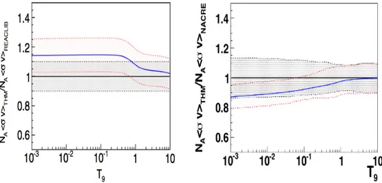
NA < σv >T HM = NA< σv >REACLIB ·fcorr (2.19) where fcorr(T9) = 1.09− 0.48 × 10−1· lnT9− 0.50 × 10−2· (lnT9)2 +0.38_{× 10}−2 · (lnT9)3 + 0.99× 10−3· (lnT9)4 +0.68_{× 10}−4 · (lnT9)5

(36)

with T9 temperature in billions of Kelvin.

Fig.?? shows the relative trend of the two reaction rates: the TH one is more efficient and deviates by ∼15% at T9 = 10−3 and by

∼5% at T9 = 1 with respect to the JINA REACLIB rate.

I updated the FRANEC reaction rate by introducing the TH cor-rection factor, as in Eq.(2.19).

• 7_Li(p,α)4_He

The 7_Li(p,α)4_{He cross section at astrophysical energies has been}

obtained from Lamia et al. (2012) by applying the Trojan Horse Method to the2_H(7_{Li,αα)n QF-reaction, using}2_{H as a TH-nucleus.}

The TH reaction rate can be written by introducing a correction factor fcorr in the analytical expression given in the NACRE

com-pilation (Angulo et al.1999):

NA < σv >T HM = NA< σv >N ACRE ·fcorr (2.20)

where

fcorr(T9) = 0.966− 0.184 × 10−1· lnT9+ 0.545× 10−3· (lnT9)2

with T9 temperature in billions of Kelvin.

Fig.?? shows the relative trend of the two reaction rates: the TH one is less efficient and deviates by ∼13% at T9 = 10−3 and by

∼5% at T9 = 1 with respect to the NACRE rate.

I introduced the TH correction factor in the FRANEC code, as in Eq.(2.20).

(37)

Figure 2.4: Left. From Lamia et al. (2013). The solid blue line rep-resents the trend of the ratio between the adopted THM 6_Li(p,α)3_He

reaction rate and the rate reported in the JINA REACLIB (Cyburt et al.2010). The red dashed line shows the upper and lower limits for the TH rate, the black dashed area indicates the upper and lower limits of the JINA REACLIB rate with the same uncertainties given in the NACRE compilation (Angulo et al.1999). Right. From Lamia et al. (2012), the solid blue line represents the trend of the ratio between the adopted THM 6_Li(p,α)3_{He reaction rate and the rate reported in the}

NACRE compilation (Angulo et al.1999). The red dashed line shows the upper and lower limits for the TH rate, the black dashed area in-dicates the upper and lower limits of the NACRE rate.

(38)

CHAPTER

3

The lithium problem

Theoretical predictions from the Standard Stellar Models1_(SSMs)

tell us that during the PMS stages low-mass stars (M_{≤ 1.3 M}⊙)

are fully convective or have deep convective envelopes . As a consequence of the PMS contraction, their interiors heat up and when the temperature at the base of the convective zone, TBCZ,

reaches that of Li burning, TLB ∼ 2.5 × 106 K, lithium is here

destroyed via (p,α) reactions. Convection is then responsible for the observed lithium depletion, by bringing the processed mate-rial to the stellar surface and the not yet processed one to the inner regions.

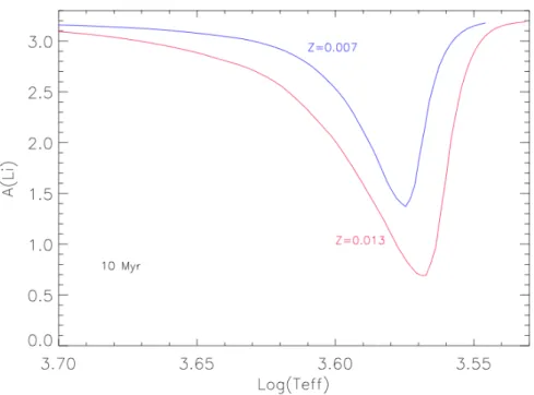
The efficiency of this process strongly depends on stellar metal-licity and mass. Li-burning is faster in metal-rich stars, since the higher opacity and the consequent deeper convective envelope re-sult in a higher TBCZ. This statement is well shows in Figure

??: at a fixed age (10 Myr), the predictions from two different classes of models for the logarithmic surface7_{Li abundace of PMS}

1_{Standard Stellar Models assume a spherically symmetric structure and}

(39)

Figure 3.1: At the age of 10 Myr, the logarithmic surface 7_Li

abun-dances are plotted for PMS stars with masses between 0.2-2.5 M⊙ and

different metallicity. Any star is identified by its effective tempera-ture, Teff. The two set of models have been computed with the same

mixing-length parameter value α=1.74 and Trojan Horse reaction rates for reactions involving lithium.

stars are plotted. Any star is identified by its effective temper-ature. The two set of FRANEC models have been computed in the mass range 0.2 - 2.5 M⊙ with the same input physics, but for

metallicity.

As to the mass, when a fully convective PMS stars (M_{≤ 0.4 M}⊙

for solar metallicity) reaching TLBit completely destroyed the

ini-tial lithium content in few tens-hundreds of Myr (see e.g. Sestito et al. 2008 and reference therein, Tognelli et al. 2015) in depen-dence on the mass: the smaller the stellar mass, the greater the time to reach TLB, the longer the timescale of Li-burning phase.

(40)

grows up as faster as larger is the stellar mass. As a consequence the convective envelope becomes progressively less extended until TBCZ < TLB and the Li-burning is stopped.

It is therefore clear how, for a fixed metallicity, the photospheric lithium content of PMS late-type stars is related to their mass and age. This has been confirmed by the large amount of7_Li

ob-servations collected for isolated stars, binary systems, and open clusters, from pre-MS to the late-MS phase (see e.g. Sestito & Randich, 2005), that showed the strong dependence of 7_Li

deple-tion on mass and age. Then, in principle, the observed surface lithium abundance can be used to derive their (lithium) age, if metallicity and mass are known, by means of theoretical evolu-tionary models.

Unfortunately, despite the well known capability of the current stellar models in reproducing the main evolutionary parameters, up to now comparison between theoretical lithium predictions and observational data may be not in good agreement (Tognelli et al. 2012, hereafter T12, and references therein). This disagreement, refers to the lithium problem, is present in both PMS and MS stars. See, e.g., the case of Pleiades (Fig.3.1), for which the large lithium dispersion observed for stars with (same) effective tem-perature Teff <T⊙is not reproduced from models (T12; Somers &

Pinsonneault 2014a,b, hereafter SP14a,b). Moreover theoretical predictions for PMS lithium depletion from SSMs tend to under-estimate the observed one, while the opposite trend is found for MS stars (Jeffries 2000;T12).

The match between lithium theoretical prediction and observa-tions for MS stars is worst and several authors claimed the in-troduction in the models of not standard physical mechanisms,

(41)

3.1. LITHIUM AND AGE OF PMS STARS

Figure 3.2: From Somers & Pinsennault 2014. Observed (dots) lithium for Pleiades, Hyades and M67 are compared to Standard Stellar Model lithium patterns (solid lines). SSMs under-predict the lithium abun-dance for the PMS stars (Pleiades), and over-predict the oldest one.

as rotationally induce mixings, magnetic fields, etc. (Tognelli et al. 2012 and reference therein). For PMS stars the situation appears better; in general the agreement between theory and ob-servations can be obtained just tuning the external convection efficiency, which often results to be less efficient than in MS stars (Tognelli et al. 2012).

3.1 Lithium and age of PMS stars

Keeping this in mind, in my thesis I test the present capability of lithium to provide an estimation of the age for a sample of PMS stars.

In principle, by exactly knowing metallicity and mass of a star, the values of a set of observational quantities (as effective temper-ature, surface gravity, luminosity, radius) and the observed pho-tospheric lithium abundance, it’s possible to compute the model with the known values of metallicity and mass. Then, one can search into this model for the age at which the values of the ob-servational parameter appear all together (theoretical age) and, independently, for the age at which the observed surface lithium

(42)

value appears in the model (lithium age). However, all the pa-rameters (including metallicity and mass) are affected by errors and one may be in a mistake in choosing exactly the estimated mass and the central value of the observed quantities. There-fore, in order to taking into account all these uncertainties at the same time, I have applied a Bayesian analysis for deriving theo-retical estimation for mass (Mmod) and age (τmod) (J¨orgensen &

Lindegren 2005 hereafter JL05). From the resulting model I have derived the lithium age related to the observed lithium abundance and compared it with the theoretical one.

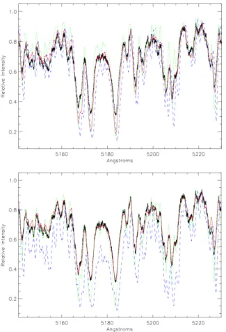
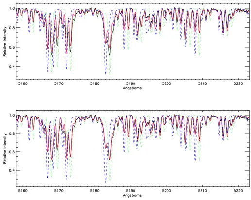
In the comparison between observational data and theoretical pre-dictions a fundamental role is given of course by the reliability of the values to be compared. From the observational point of view, the measurements are often largely uncertain, because of the de-pendence on other observational quantities and so approximated estimation (i.e., the absolute magnitude depends on the assumed distance) and/or because of the instrumental limits (e. g., low-resolution spectroscopy). Fig. 3.2 shows the case of the binary system V773 Tau A. Boden et al. (2007) carried out a spectro-scopic determination of effective temperature and surface gravity for both components, from a spectrum with resolution R=35000. However, Kurucz synthetic spectrum as computed by assuming the authors results doesn’t match the high resolution (R=115000) high signal-to-noise (S/N = 68) HARPS-North spectrum.

From the theoretical point of view, it has to be noted that the adoption of different physical inputs (such as equation of state, radiative opacity, nuclear cross sections, convection efficiency, etc) in computation of stellar evolutionary models lead to different pre-dictions for surface lithium abundance at a fixed mass and age. In particular, the convection efficiency in super adiabatic regions (i.e. the mixing length parameter) and the cross sections for

(43)

nu-3.1. LITHIUM AND AGE OF PMS STARS

clear reactions involving lithium are fundamental ingredients to obtain reliable theoretical predictions. An example is showed in Fig. 3.3: the logarithmic surface 7_{Li abundace is plotted at a}

fixed age (∼10 Myr) by means of two classes of models with solar metallicity and mixing length parameter α=1 (in red) and 1.74 (in purple). Each class has been computed with the same as-sumptions on the adopted input physics, but for nuclear reaction rates for reactions involving lithium, that are from Trojan Horse (empty circles) and NACRE compilation (filled circles).

A constraints for theoretical model results are the binary systems, which have same metallicity and age. Bayesian determinations of stellar mass and age has yet been successfully applied by Gen-naro et al. (2012, hereafter GPT12) to a sample of stars includ-ing detached, double lined, eclipsinclud-ing (EB) binaries, astrometric-spectroscopic (AS) binaries and astrometric-spectroscopic binaries with cir-cumstellar disk (DSK). These classes are the only for which the dynamical mass (Mdyn) of both components are determined. Mdyn

is distance-independent, then it represent a reliable observational estimation, useful in deriving theoretical bayesian results.

Unfortunately the number of known objects belonging to these classes and for which lithium surface abundance is available is small. Anyway, since the radial velocities are nowadays between the most accurate measurements, I suggest to enlarge the sample by applying the method to PMS double lined spectroscopic bi-naries (SB2) by means of the mass-ratio of the two components, which directly follows from their radial velocities.

The use of mass-ratio, however, doesn’t allow to derive the age of each star, but only provides an estimation for the age of the system (coevality). Anyway, the hypothesis of coevality is a good assumption for a binary system.

(44)

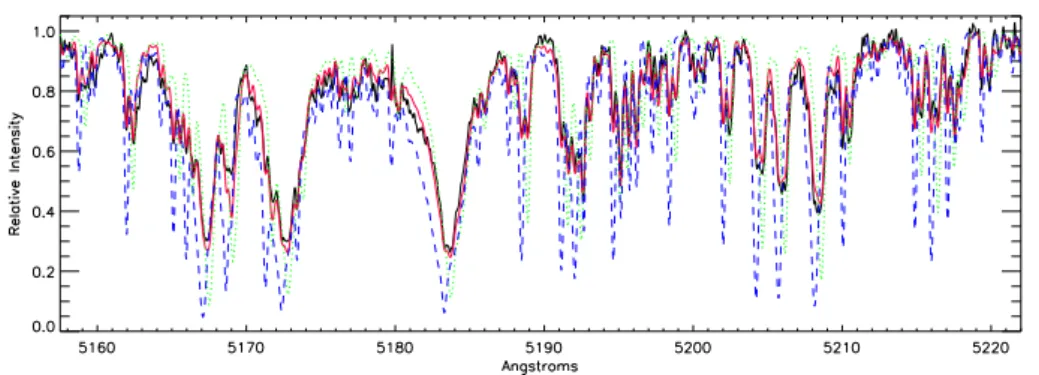
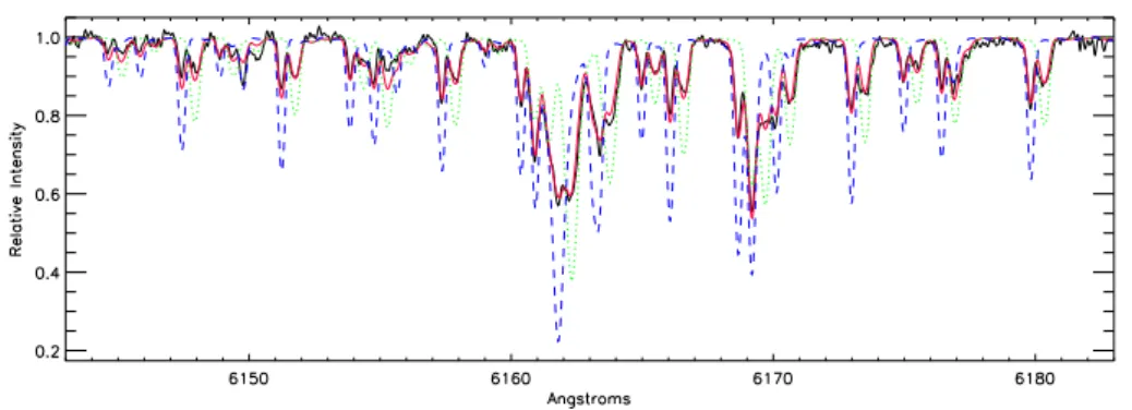
Figure 3.3: U pper panel: HARPS-North spectrum (R=115000, S/N=68) of the binary system V773 Tau A and synthetic one (red) computed with no veiling, Teff=4900 and 4700 K and logg=3.9 and

4.1 for primary (green) and secondary (blue) component respectively. These values have been determined by Boden et al. (2007) from spec-troscopy at R=35000, S/N =35. - Lower panel: synthetic spectrum computed with a veiling of 15%, Teff = 4700 and 4100 K and logg =

3.7 and 3.7 for primary and secondary component fits the observed one at the best.

(45)

Figure 3.4: Logarithmic surface 7_{Li abundace is plotted against T} eff,

at the same age, for two classes of models with solar metallicity and mixing-length parameter α=1 (purple), α=1.74 (red). Each class has been computed with different inputs for cross sections of reaction in-volving lithium, i.e. THM (empty circles) and NACRE (filled circles).

(46)

CHAPTER

4

Stellar evolution modeling

4.1 Stellar structure equations

A star can be defined as a self-gravitational gaseous structure in hydrostatic equilibrium. Under the assumption of spherical symmetry and by neglecting the effects of magnetic fields as a first approximation, the internal stellar structure is described by the following system of four differential equations (see, e.g., Castellani 1985): dP dr = − GMrρ r2 (4.1) dMr dr = 4πρr 2 _(4.2) dLr dr = 4πϵρr 2 _(4.3) dT dr = f (Mr, r, Lr, T, P) (4.4) where

(47)

4.1. STELLAR STRUCTURE EQUATIONS

– P is the total pressure

– Mr is the mass contained inside a shell of radius r

– Lr represents the energy through a surface of radius r (it

indicates the luminosity when r is equal to the stellar radius R)

– T is the gas temperature

– the function f (Mr, r, Lr, T, P) defines the temperature

gra-dient in each region of the star depending on the energy transport mechanism (i.e. radiative/convective heat trans-port).

– ρ is the gas density

– ϵ represents the total energy production per gram and per second

Density and energy production are functions of r, Mr, P , T and

Lr. Generally the mass M is assumed as independent variable,

so that the unknowns are the four quantities P , T , r and L.

The solution of the system allows to derive the trend of the quan-tities characterizing stellar interiors as a function of the mass and for a fixed chemical composition, then representing a powerful tool to explore stellar structure and evolution. This is what stel-lar evolutionary codes do.

In order to solve the equations system, a code needs the following input physics:

– Equation of state, which provides all the thermodynamical quantities required for the integration of a model, such as the density ρ, specific heat at a constant pressure cP , molecular

weight µ, and the adiabatic gradient ∆ad

– Radiative and conductive opacity coefficients. The opacity coefficients determine the transparency level of the stellar

(48)

gas to the energy transport.

The radiative opacity, due to the interaction between radia-tion and matter, depends on several photon absorpradia-tion pro-cesses or scattering on molecules, atoms, ions, or electrons present in the stellar gas. Although the most of these pro-cesses strongly depend on the frequency, stellar evolutionary codes make use of a mean value (Rosseland mean opacity) obtained by averaging the frequency-dependent opacity over the frequency distribution (approximated to a black body). The conductive opacity is related to the electron conduc-tion, which is not negligible when the free electron densities are high and the electrons begin to become degenerate. It mainly regards (low mass stars) and stars in more advanced post-main sequence phases.

– Energy production. The total stellar energy production co-efficient can be written as the sum of three quantities

ϵ= ϵg+ ϵn− ϵν (4.5)

where the first term is related to the energy generated by thermodynamical transformations of the gas (gravitational energy), the second one indicates the energy production by nuclear burnings and the third (important in post main-sequence phases) represents the energy-loss due to thermo-neutrinos, that are neutrinos produced not in nuclear fusions (i.e. photon-, pair-, and bremsstrahlung- production). together with the convection treatment, which is the formalism adopted to treat the convective heat transport inside a star and in particular in the outermost stellar envelopes, and the boundary conditions, that are the physical quantity values at the stellar center and surface. Of course, at the center of a star (M = 0) the boundary conditions can be expressed by setting both radius and luminosity equal to zero, so that r(M = 0) = L(M = 0) = 0.

(49)

For what concerns stellar surface, the usual approach consists in adopting the physical quantities at the base of the atmosphere as boundary condition values.

For this work, I have computed a database of stellar models by means of the Frascati Raphson Newton Evolutionary Code (FRANEC, Degl’Innocenti et al. 2008). The models have been evolved from the early PMS phase up to the end of the central MS H-burning and however not longer than an age of 20 Gyr. FRANEC solves the set of equations by considering two stellar re-gions: the interiors (from the center to a fraction of the total mass ∼99.98%) in which the mass is adopted as independent variable, and the sub-atmospheric region, which represents the remaining ∼0.02% of fractional mass and where the adopted independent variable is the total pressure. The integration procedure adopted by the code is briefly described below.

– Computation of a starting model through the fitting method, which consists, given four boundary conditions, two at the surface (luminosity and effective temperature), and two at the center (central pressure and temperature), in integrating the stellar structure equations from the surface downward and from the center upward. The interior and exterior solu-tions have to match in a given point, the fitting point. With an iterative procedure, the four boundary conditions are ad-justed until the convergence at the fitting point is achieved within a specified tolerance.

Such a model represents the one at time zero (t = 0). – Evolution. The model obtained from the fitting method (t =

0) or the model computed for each time-step (t̸= 0) is then evolved. The evolution consists in computing the structure at the next time-step t + ∆t, where t is the age of the current model. The time does not appear explicitly in the structure equations, given the hydrostatic nature of the code, but it