Campus di Cesena - Scuola di Scienze
Corso di Laurea in Scienze e Tecnologie Informatiche
Design and Implementation of a Testbed
for Data Distribution Management
Tesi di Laurea in Reti di Calcolatori
Relatore
GABRIELE D’ANGELO
Presentata da
FRANCESCO BEDINI
II Sessione
Anno Accademico 2012 - 2013
and is immortal.” - Albert Paine
Data Distribution Management (DDM) is a core part of High Level Archi-tecture standard, as its goal is to optimize the resources used by simulation environments to exchange data. It has to filter and match the set of informa-tion generated during a simulainforma-tion, so that each federate, that is a simulainforma-tion entity, only receives the information it needs. It is important that this is done quickly and to the best in order to get better performances and avoiding the transmission of irrelevant data, otherwise network resources may saturate quickly.
The main topic of this thesis is the implementation of a super partes DDM testbed. It evaluates the goodness of DDM approaches, of all kinds. In fact it supports both region and grid based approaches, and it may support other different methods still unknown too. It uses three factors to rank them: execution time, memory and distance from the optimal solution. A prear-ranged set of instances is already available, but we also allow the creation of instances with user-provided parameters.
This is how this thesis is structured. We start introducing what DDM and HLA are and what do they do in details. Then in the first chapter we describe the state of the art, providing an overview of the most well known resolution approaches and the pseudocode of the most interesting ones. The third chapter describes how the testbed we implemented is structured. In the fourth chapter we expose and compare the results we got from the execution of four approaches we have implemented.
ddmtestbed/. It is licensed under the GNU General Public License version 3.0 (GPLv3).[11]
Questa tesi tratta di diversi aspetti riguardanti il Data Distribution Man-agement (DDM), nell’ambito degli ambienti di simulazione distribuiti ader-enti allo standard High Level Architecture (HLA).
Il DDM si occupa di gestire la trasmissione dei messaggi tra i vari ambi-enti di simulazione, chiamati federati. Il suo compito `e quello di ottimizzare le risorse di rete, facendo in modo che vengano trasmesse soltanto le in-formazioni veramente necessarie ai vari federati, in modo che non vengano saturate.
Abbiamo sviluppato un testbed in C per la valutazione degli approcci di risoluzione in quanto, al momento, non `e liberamente disponibile alcun software super partes riguardante questo campo di ricerca.
La tesi `e cos`ı strutturata: nei primi due capitoli `e descritto lo stato dell’arte, introducendo il DDM e HLA ed evidenziando con particolare cura i pro e i contro di ogni approccio di risoluzione, fornendo lo pseudocodice dei principali. Il capitolo 3 descrive come `e stato implementato il testbed per la valutazione di quest’ultimi. Nel quarto capitolo vengono esposti e confrontati i risultati ottenuti dall’esecuzione di quattro diversi approcci di risoluzione noti in letteratura da me implementati secondo le specifiche del testbed. Questi sono stati poi valutati utilizzando istanze con diverse pecu-liarit`a e dimensioni.
1This section was added to fulfil “Universit`a di Bologna”’s requirements for non-Italian
thesis. The rest of the thesis is written in English.
idioma, la lingua de facto dell’informatica e delle pubblicazioni scientifiche. `
E infatti l’unica che pu`o essere utilizzata per predisporre e consentire la massima diffusione dei risultati scientifici ottenuti.
Abstract . . . I Prefazione . . . IV Table of Contents . . . VI List of Figures . . . VII List of Tables . . . IX 1 Introduction to DDM 1
1.1 High Level Architecture . . . 1
1.1.1 Version History . . . 2
1.1.2 HLA Structure . . . 2
1.2 Data Distribution Management . . . 3
2 The State of the Art 5 2.1 How Information are Matched: the Routing Space . . . 6
2.2 Matching Approaches . . . 7 2.2.1 Region-based Approaches . . . 8 2.2.2 Grid-Based . . . 12 2.2.3 Miscellaneous Approaches . . . 13 2.3 Summary . . . 15 3 The Testbed 17 3.1 The Testbed’s Goals . . . 17
3.2 The Testbed Structure . . . 18
3.3 DDMInstanceMaker . . . 19
3.3.1 DDMInstanceMaker parameters . . . 19 V
3.4 DDMBenchmark . . . 26
3.4.1 DDMBenchmark parameters . . . 27
3.4.2 Evaluation Criteria . . . 27
3.4.3 How the score is computed . . . 32
3.4.4 How to Implement an Approach . . . 34
3.5 Summary . . . 36 4 Implementation Results 39 4.1 DDM Instances . . . 40 4.2 Results . . . 40 4.3 Tables . . . 53 5 Conclusions 59 5.1 Future Works . . . 61 A Approaches Implementations 63 A.1 Brute Force . . . 63
A.2 Sort Based . . . 64
A.3 Binary Partition Based . . . 65
B Testbed highlights 67 B.1 compile.sh script . . . 67
1 DDMTestbed download link . . . II
2.1 Update and subscription extents inside a 2D routing space. . . 6
2.2 Extents edges projection on a given dimension. . . 9
2.3 Binary partition on a given dimension . . . 12
2.4 Comparison between grid-based cells size . . . 14
3.1 Overflow handling . . . 27
3.2 Detailed result example . . . 33
3.3 Rank file example . . . 34
4.1 The profiler result . . . 50
2.1 Approaches comparison . . . 16
3.1 Default Instances . . . 20
3.2 Truth tables . . . 28
3.3 Scripts . . . 36
4.1 Results of optimal approaches - Part 1/2 . . . 54
4.2 Results of optimal approaches - Part 2/2 . . . 55
4.3 Results of approximated approaches - Part 1/3 . . . 56
4.4 Results of approximated approaches - Part 2/3 . . . 57
4.5 Results of approximated approaches - Part 3/3 . . . 58
Introduction to Data
Distribution Management
This chapter explains what Data Distribution Management (DDM) is and why it plays a major role in distributed simulations. To do so we’ll need to quickly explain what is High Level Architecture, the architecture whose DDM belongs to. Afterwards we describe different approaches and algorithms that have been created during the last 15 years to handle DDM.
1.1
High Level Architecture
High Level Architecture (HLA) is a distributed computer simulation stan-dard that allows interoperability between heterogeneous simulation systems.[1] Nowadays simulations can be so high detailed that they can’t be executed on a single machine any longer. Many computers can be linked together via a computer network, forming a cluster, and exchanging information and state updates. HLA ensures that simulation environments built by different manufacturers are able to communicate one another using a common set of rules and protocols.
1.1.1
Version History
The U.S. Department of Defense (U.S. DoD) Architecture Management Group (AMG), under the leadership of the Defense Modeling and Simulation Office (DMSO), started developing HLA baselines in 1995. These baselines were approved by the U.S. Department of Defense in 1996.[23] The first complete version of the standard was published in 1998 and was known as HLA 1.3. It was later standardized as IEEE standard 1516 in 2000[1].
The most recent version of the standard was published in 2010 and it includes the current U.S. DoD standard interpretations.[2]
1.1.2
HLA Structure
HLA is made up of 3 components:
Interface specification: Defines how HLA compliant simulation environ-ments interact using a Run-Time Infrastructure (RTI). RTI is a sup-porting software that consists of an implementation of six groups of ser-vices (whose complete implementation is not compulsory), provided as programming libraries and application programming interfaces (APIs), as defined by the HLA specifications.
Object Model Template (OMT): It states what information are exchanged between simulations and how they are documented.
Rules: Simulations must obey to these rules to be HLA compliant.
In HLA technical jargon, every simulation environment is known as a federate, whereas a collection of federates sets up a federation.
This is all you need to know to understand the topics discussed in the rest of this thesis. Now we can start to introduce the main argument of this thesis: Data Distribution Management.
1.2
Data Distribution Management
A centralized simulation would have full access to the system memory assigned to its process, and so all information are fully available to each task. In a distributed environment, federates would certainly need to exchange information too. This is where Data Distribution Management comes in.[16] DDM is the service included in RTI that provides a scalable, efficient mechanisms for distributing information between federates. Its task is to handle data transmission and state updates that are sent between the various simulations. Its goal is to optimize the available resources, that is minimizing the volume of data transmitted over the network that links the federates together.
In fact it’s very common that a federate only needs a subset of all the available data. For example, if we had a federation that is simulating traffic flow in a big metropolis or in an entire nation, we probably would have a federate that simulates the state of all the traffic lights located in the case in question. A travelling car would only be interested to the state of traffic lights place in the upcoming intersections. The state of all the other traffic lights would be completely irrelevant to that car’s driver.
Federates during each message exchange can be divided in two groups: the ones that publish information, called publishers, and the ones that want to receive that information, called subscribers. DDM has to match their transfer intents in an optimal way in order to minimize network’s usage.
On each transmission session DDM goes through the following steps: 1. Subscribers declare what information they want to receive, publishers
declare what information they intend to send.
2. A matching algorithm detects the intersections between these transfer intents.
3. All subscribers that match with a certain publisher must receive data from the relative publisher. In some implementations,[15] this is achieved
creating multicast groups.1
4. Publishers send their data via their multicast group. Subscribers may need to execute an additional filtering to select the information they wanted.
The final filtering is only necessary if the matching algorithm is not op-timal, that is when is allowed to obtain false positives in the result (i.e. solution provided is sub-optimal). This can be allowed, in certain circum-stances, when a limited amount of superfluous data entails an improvement in the computational complexity of the matching algorithm.
The opposite case is not allowed; all the matching intents has to be de-tected by the matching algorithm, otherwise at least a subscriber won’t re-ceive at least a chunk of information it has legitimately requested.
1Multicast groups allows one-to-many communication over an IP infrastructure. The
The State of the Art
If DDM would not be implemented by RTI, the only way to ensure that each subscriber would receive all the data it needs is that all publishers would send their data to each subscriber. Every subscriber then would waste time filtering the required data by itself, moreover a lot of network bandwidth would be wasted. It’s trivial to see that this method is completely inefficient as it allows to a huge amount of useless data to occupy network’s resources. Let n, m be the number of publishers and subscribers respectively. The amount of data that is transmitted over the network can be quantified as:
n
X
i=0
DataSize(i) ∗ m
This would quickly saturate network’s resources when the number of federates increases.
In order to overcame this waste of resources, many DDM approaches have been developed in the last 15 years. The following sections describe the most well-known.
2.1
How Information are Matched: the
Rout-ing Space
In order to declare what information publishers intend to transmit and subscribers intend to receive, federates generate extents on a routing space. A routing space is a multidimensional coordinate system whereon the sim-ulation takes place. Federates create extents on it to indicate the area they want to receive/provide information. An extent is a rectangular subspace of the routing space; a group of extents sets up a region.1 Regions submitted by publishers are called update regions, regions submitted by subscribers are named subscription regions.
When a subscription region is superimposed to an update region, the subscriber which made the subscription must receive data from the relative publisher.
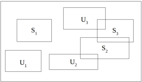
Figure 2.1: Update and subscription extents inside a 2D routing space. Figure 2.1 shows three update extents (marked with a capital U) and three subscription extents (marked by a capital S) placed inside a bidimensional
1It is common practice to consider a region as an indivisible part, making the terms
routing space. U1 and S1 are not overlapped to any other extent, hence they
shouldn’t send nor receive any data in this session. On the other hand, U2 is
superimposed to S2 whereas U3 is overlapped to S3. This means that U2 will
send data to S2 as U3 will provide data to S3. The fact that S2 is overlapped
to S3 is not to be taken into consideration by the matching algorithm as
two subscribers don’t exchange data one another. This would apply to two update extents too.
For example, we could simulate smartphones’ GPS and network reception in a certain area using a 3D routing space. Two dimensions would be used to indicate the position of the smartphones and of the the antennas and GPS satellites, whereas the third would be used to distinguish between between GPS and network coverage. Hence we can treat smartphones as subscribers and the antennas and satellites as publishers. Update extents would represent the coverage area of the publishers whereas the subscription extent would represent the signal strength of the subscribers. When a publisher extent overlaps an update extent the relative mobile phone is considered able to communicate with the relative cell or satellite.
2.2
Matching Approaches
Matching approaches are mainly divided in two categories: grid-based and region-based approaches. In the following sections we’ll describe the most relevant ones. These two categories are not mutually exclusive; they can be combined to appraise their strong points and lessen their weak points. In the following sections, when it will be possible to state the computa-tional cost of an approach, it will be shown consistently using n, m as the number of publishers and subscribers respectively and d as the number of dimensions.
2.2.1
Region-based Approaches
Region-based approaches require that a centralized coordinator compares extents one another, or that each federate compare its extents with the one generated by the others. Region Based approaches usually have a higher computational cost than Grid-based approaches, but they tend to generate less false positives than Grid-based ones (in fact most of them provide an optimal solution).
2.2.1.1 Brute Force
This approach performs all the possible comparisons between every up-date extent and each subscription extent. If two extents are superimposed on every dimension they are considered matched.
Pro: Easiness of implementation, straightforward, provides an optimal so-lution.
Cons: Not scalable; this method produces the maximum number of com-parisons.
Let m be the number of subscribers’ extents and n the number of publishers’ extents. Computational complexity of the brute force approach is:
Θ(d · (m · n))
The pseudocode of a possible implementation of this approach can be found in section A.1 on page 63.
2.2.1.2 Sort Based
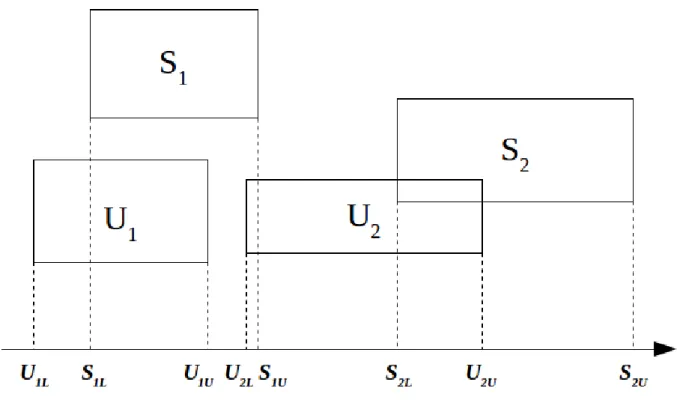
This approach lowers the number of comparisons ordering the extents’ edges.[20] Sort based method works on a dimension at a time, projecting extents’ bounds on each dimension as shown in figure 2.2. We recall that an extent is considered matched to another if and only if is matched on every dimension.
According to this approach a vector for each dimension is created. It contains the relative extents’ edges in a given dimension. Hence edges are sorted and read sequentially.
Figure 2.2: Extents edges projection on a given dimension.
This approach takes advantage of the ordered relation that states that an extent can only precede, include or follow another extent. When we extract edges from the list we can obtain a subscription or an update edge. We can keep trace of the state of the subscription extents using two lists so defined: SubscriptionSetBefore: contains all the subscription extents that are al-ready ended (whose upper edge has alal-ready been pulled out from the vector).
SubscriptionSetAfter: contains all the subscription extents that follows (whose lower edge has not been extracted from the vector yet).
When we extract an edge that is part of an update extent we can draw some conclusions analysing the state of the two lists just described. If we extract the lower bound we can state that all the subscribers in the Subscription-SetBefore are not overlapped to the current update extent, whereas if we extract an upper bound we can say the same for the subscribers that are still in SubscriptionSetAfter.
As scanning the vectors has a linear cost, sort based computational com-plexity depends on the sort comcom-plexity. If we use Introspective sort algo-rithm2 we could consider it linearithmic in the number of edges[17], hence
we get:
Θ(d · ((m + n) · log(m + n)))
Pro: The number of comparison is lowered compared to the brute force approach, so it’s more scalable.
Cons: It requires a little more memory to perform matching (as d additional vectors has to be stored).
Algorithm A.2 on page 64 shows a possible sort based implementation. 2.2.1.3 Binary Partition
This method uses a divide et impera approach, similar to the one adopted by the Quicksort algorithm.[13] As well as the sort based, also binary partition approach examines one dimension at a time. Edges are then sorted and recursively binary partitioned using the median as the pivot value. We obtain two subsets so defined:
Left (L): A set that contains all the extents that terminates before the pivot value.
Right (R): A set that contains all the extents that begin after the pivot value.
2Introspective sort is an improved version of the Quicksort algorithm that has a
This partition would not be complete as it not includes the extents that include the pivot value. We call this group of extent P. These are unnaturally included in the L partition, even if they don’t strictly belong to it. The key factor of this approach is that the extents that belong to this P partition are automatically considered matched as they share a common value. The next step involves the following comparisons:
• L subscription extents with P update extents • L update extents with P subscription extents • R subscription extents with P update extents • R update extents with P subscription extents
After this L and R are recursively partitioned until their both empty. Considering that the computational cost depends on the extents distri-bution in the routing space, it’s difficult to estimate its cost. As the vec-tors are initially sorted, as for the sort based approach, the cost would be ω(d · (n + m) · log(n + m)).
This algorithm works better if the pivot falls in zones where most extents overlaps, as comparison cost is lowered this way. The opposite case is not dramatic either, as the four comparison would not take place if the P partition would be empty. The worst case (i.e. the highest number of comparisons) happens when L, R, and P have a similar size.
Figure 2.3 on page 12 shows a partition example. Extents S1 and U2 are
placed in the L partition as they end before the pivot value. Extent S6 is
placed on the R partition as it begins after the pivot. Extent U3, S4 and S5
are placed in the P partition as they include the pivot value. We get, at no cost, that U3, S4 and S5 are overlapped on the given dimension. The next
step is to check whether S1 is superimposed to U3, if U2 is overlapped to S4
or S5, etc. (i.e. the same goes for the extents in the R set).
Figure 2.3: Binary partition on a given dimension
approach. It works best in clustered instances, as more extents would fall in the P partition.
Cons: More complicated data structures has to be stored. If partition isn’t performed in place six vectors (three for the subscribers, and three for the publishers) has to be allocated on each node of the recursion tree. The pseudocode of a possible implementation of this approach can be found in section A.3 on page 65.
2.2.2
Grid-Based
Grid-based approaches treat the routing space as a chessboard, that is they divide it in a grid of cells. An extent can lay on one or more contiguous cells. Approaches that belong to this categories tend to be less restricting than region-based ones, wasting more network bandwidth. Their advantage is that their computational cost is often lower.
One of the most important element for the success of these approach is to correctly set the size of the cell, in fact this is a key factor and many studies
has been carried out about this topic.[5, 21] Smaller cells bring a higher level of precision in matching detection but they involve the use of more resources during the execution of the matching algorithm. Bigger cells, on the other side, require less matching resources but tend to provide worse results. 2.2.2.1 Static Approach
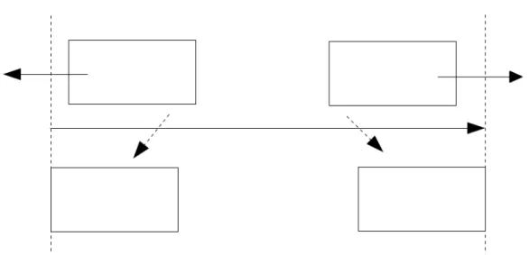
Static approach (also known as Fixed Approach) is the most straightfor-ward grid-based approach. It just considers matched two extents if they lay, even partially, on the same cell. This means that two extents might not be superimposed at all, anyway they would be considered matched if they occupy the same cell, causing the generation of false positives.
There is a multicast group preallocated for each cell. Publishers and sub-scribers join a group if one of the extents they generated lays even partially on the relative cell. This means that publishers who are the only federates in a cell would send data even if there is nobody to receive it in that multicast group.[7]
Figure 2.4 shows how crucial can the dimension of the cells be when using this approach. In figure 2.4(a) small cells are used, whereas in figure 2.4(b) bigger cells are shown. Applying the static grid-based approach, it’s easy to see that the number of false positive increases as the area of the cells grows (see fig.2.4(c) and 2.4(d)).
Pro: No matching performed.
Cons: Lots of wasted bandwidth, depending on the size of the cells and the extents.
2.2.3
Miscellaneous Approaches
This section reports three approaches that don’t lay completely in the previous categories, as they try to get the best from both.
(a) Small cells (b) Large cells
(c) Matches detected using small cells (d) Matches detected using large cells
Figure 2.4: Comparison between large and small grid cells. A dashed arrow indicates an erroneous match whereas a plain one shows a correct match. 2.2.3.1 Hybrid Approach
This kind of approach, in some situation, “can reduce both the number of irrelevant messages of the grid-based DDM and the number of matching of the region-based approach”.[22] It consists in applying a static grid-based and then filtering the result using the brute force region-based approach. This allows to reduce the complexity of the brute force algorithm and decrease the number of false positives identified by the static grid-based approach.
It’s possible to use other region-based approaches to improve the last filtering. When the number of matched extents detected by the static grid-based approach is high enough to justify the overhead of more complex data structures, a more sophisticated approach should be used.
Pro: The second filtering permits to reach an optimal solution. Cons: Its efficiency depends on the grid size.
2.2.3.2 Grid-filtered region-based
This approach is very similar to the Hybrid Approach described in the previous section. The difference is that the region-based matching is not performed on any cell, but only on cells that are occupied over a certain per-centage by extents. Choosing the correct threshold is as thorny as choosing the best cell size in a grid-based approach.[6]
This method should be used when networks’ resources are highly available and a limited amount of false positives can be acceptable.
Pro: It performs less matching than the other miscellaneous approaches. Cons: Produces false positives. It has to be fine-tuned choosing the right
cell size and threshold based on the given instance. 2.2.3.3 Dynamic Approach
Each federate is the owner of one or more cells and knows every sub-scribers’ and publishers’ related activity. This makes a central coordinator unnecessary.
When the owner detects a match it allocs the relative multicast group and notifies the involved extents.[7]
Pro: Distributed, more efficient than grid-based, the second filtering permits to reach an optimal solution.
Cons: Its efficiency depends on the grid size.
2.3
Summary
In this chapter the most well-known matching approaches have been anal-ysed. Table 2.1 shows a quick view of the properties of the approaches we
Table 2.1: Approaches comparison
Approach Matching Performed Distributable Optimal Match Static Grid-Based X Brute Force X X X Sort Based X X Binary Partition X X Hybrid X X Grid-Filtered X X Dynamic X X X described.
There is a huge variety of different approaches, and establishing which one works best on a given instance it’s not so obvious. Choosing the right cell size in grid-based approaches is a key factor that can’t be underrated. The testbed we implemented wants to be useful in making clear when it’s convenient to use a certain approach instead of another.
The Testbed
This chapter explains how the testbed was designed and projected. We start by explaining the testbed’s goals, then we proceed explaining its struc-ture and describing in detail how it is strucstruc-tured and how its components work.
At the end of this chapter, an explanation about how to implement an approach on our testbed can be found.
3.1
The Testbed’s Goals
We wanted to create a testbed to easily compare different approaches and different parameters within the same approach, producing a useful and handy tool that would allow researchers to focus on their innovative approach rather than losing time in implementing a new ad hoc benchmark to execute their evaluation tests.
Moreover, in some papers, it looks like authors simulate a routing space specifically built to just disclose the strong points of their algorithms, with the result that each approach is “better” than all the others.
To remove all doubt, we want to provide a standard and independent measuring instrument to compare the goodness of a proposed approach on a fixed set on instances whose solution is known. Researchers can implement
their approaches, run them on our benchmark and compare their results with the one got by other approaches already implemented. Obviously we encourage researches to share their code to perform efficiency comparisons on a wider set of resolutive methods and instances.
It is however possible to use our tool only to check for the validity of a proposed algorithm; our testbed, among other things, checks that the pro-vided solution is acceptable and returns the number of false positives if the solution is sub-optimal.
As we’re supporting OpenMP[19] too, our testbed can be used to test parallel code and easily test the solutions. Repeating the test an appropriate number of time may unmask the presence of race conditions or other parallel critical situations that randomly cause wrong results.[18]
3.2
The Testbed Structure
The testbed has been written in C (C89 ).[4] It has been mainly devel-oped using Code::Blocks open source IDE[8] running on an Ubuntu 13.04 x64 machine. We chose to use the C language to obtain top performances and full control on the generated code. As we’re working a lot on bitwise operations, we think that the C++ additional features weren’t needed.
At the beginning we tried to keep it Windows R compatible, but as
com-plexity grew we realized that this would be such a huge effort and it wouldn’t be worth it. For this reason, our code is compatible with Unix-like operating systems only.
The testbed is released under the GNU General Public License version 3 (GPLv3)[11] and can be downloaded using the link provided at the end of the abstract.
It is composed by two parts:
DDMInstanceMaker: handles the generation of the instances.
the generated instances at a time, checks for the solution validity and computes a score for the proposed resolution approach.
All the most important parts of the code has been documented using the DoxyGen tool,[9] hence it is possible to find a detailed HTML documentation attached to our project.
3.3
DDMInstanceMaker
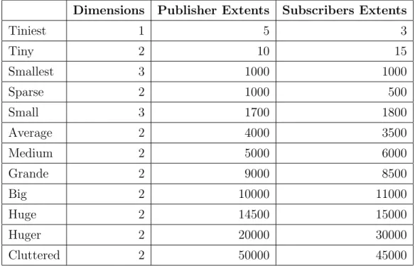
DDMBenchmark comes along with a set of instance already generated. These instances have different size and different peculiarity, so they are per-fect to deeply test a proposed method. Their characteristic are shown in details in table 3.1 on page 20.
Moreover there are some multi-step instances1 that have the same size
of their main instance, but they represent the evolution of the instance in a certain number of consecutive steps. We called them to represent their parameters’ values: for example MEDIUM20U represent a 20 step instance with the same characteristics of the MEDIUM one. The U or S at the end of the name states that update/subscriber extents stand still between all the iterations.
Of course we didn’t want to constraint the final users in using these instances only, so we created DDMInstanceMaker. It allows them to create their own instances providing a rich set of parameters.
3.3.1
DDMInstanceMaker parameters
DDMInstaceMaker accepts the following compulsory parameters:
-d number of dimensions it represents the number of dimensions that are used within this routing space. For efficiency purposes it has to be lower that the MAX DIMENSION define. This allows the proposed methods to
Table 3.1: Default Instances
Dimensions Publisher Extents Subscribers Extents
Tiniest 1 5 3 Tiny 2 10 15 Smallest 3 1000 1000 Sparse 2 1000 500 Small 3 1700 1800 Average 2 4000 3500 Medium 2 5000 6000 Grande 2 9000 8500 Big 2 10000 11000 Huge 2 14500 15000 Huger 2 20000 30000 Cluttered 2 50000 45000 partially declare their data structure statically, reducing the number of dynamic memory allocation and deallocation calls.
-u number of update extents it represents the number of update extents that will be created on this routing space.
-s number of subscription extents it represents the number of subscrip-tion extents that will be created on this routing space.
-n name of the instance it is the name of the instance the user is about to produce. It will be used to create a subfolder called like the given name that will contains all the files related to this new instance. This name has to be unique and a folder with the same name must not exist (otherwise execution will terminate with an error message). Although blank spaces are allowed, we recommend to keep this name short and to use a single word.
And these optional parameters:
-r random seed this is the unsigned int that will be used to initialize the C rand function. If not provided it will be initialized using the current timestamp.
-a name of the instance author This info will be saved as a comment inside the instance info file.
-v version number of the instance It allows you to include a version num-ber to the instance you are generating. If not provided the default value is 1.0.
-l sequence length this positive number represents the number of input instances that will be generated as consecutive steps. If not provided the default value is 1.
-R movement restrictions 0|1|2 Provided as an integer value, in case se-quence length is greater than 1, it is possible to choose to make all the extents move (0, this is the default behaviour), or to move the subscription extents only (1), or to move the update extents only (2). -S averageSize This parameters allows the user to provide the average
ex-tent size. Higher is this value more cluttered will be the result, a lower value would generate a sparser instance. If not provided the extents size will be randomly generated. DDMInstanceMaker will try to create extents whose average dimension is the provided value. We randomly generate the lower bound, then we generate a random value between [0, averageSize ∗ 2], that is the size of the extent (so upperBound = lowerBound + RandomV alue). For the law of large numbers,[10] for an infinite number of extents, the exents’ average size will tend to the expected value of the discrete uniform distribution, that is:
minV alue + maxV alue
2 =
0 + averageSize · 2
For this reason, it is inadvisable to use this parameter on really small instances, as the result may not be accurate (in the worst cases you’ll get an average size of 0 or averageSize · 2).
-k skip confirmation prompt if this parameter is provided DDMInstance-Maker executes in batch mode, without any user interaction.
-h help Provides an help screen.
DDMInstanceMaker firstly evaluates the correctness of the input parame-ters, then it generates an instance that respects the given parameters. The In-stance is resolved using the brute force algorithm described in section 2.2.1.1 on page 8, as it’s the only method known that is guaranteed to produce an optimal solution (as it performs all the possible comparisons).
For each new instance a folder called <instanceN ame> is created. It will contain the text files that stores the generated instances and the binary files that contains the optimal results.
The file that stores the info about the parameters that generated the current instance is named info.txt. We report an example of this file. 1 #I n s t a n c e name : s m a l l 2 #I n s t a n c e v e r s i o n : 1 . 0 3 #C r e a t e d on Tue Jun 11 1 5 : 1 3 : 2 8 2013 4 #Author : F r a n c e s c o B e d i n i 5 #Random Seed : 234 234234 6 #S e q u e n c e l e n g t h : 7 1 8 #D i m e n s i o n s 9 2 10 #S u b s c r i p t i o n R e g i o n s 11 5 12 #Update R e g i o n s 13 10
The lines that start with a # symbol are comments, they won’t be read by the testbed. We use the same format for the input files, the ones that contain the edge state of a given step. They are named input-i.txt, where i is an integer in the interval [0, ..., s − 1], and s is the length of the generated sequence. The same applies to the output files, which are called output-i.dat.
Here’s an example of an input-0.txt file:
1 #S u b s c r i p t i o n s <i d > <D1 e d g e s > [<D2 e d g e s > ] . . . 2 0 522225 6275355 −30396036507 7593553 3 1 −409933 −4169 −249428622392 8 3 4 2 1 6 6 0 0 2 4 2 −66112659340 1503439 −892267956 −66918 5 . . . 6 4 −89869243 4 7 9 5 2 9 5 6 8 8 −5677652 7198 7 #Updates <i d > <D1 e d g e s > [<D2 e d g e s > ] . . . 8 0 −184066 363577 −7957130 569659 9 1 −79366143 47952500 −6260736 71989568 10 . . . 11 9 −5763996 −9770 −6094673 104120
As is shown by the comments in the file, each row represent an extent. The first number represents its ID which is unique between extents of the same type. We guarantee that IDs are in the range [0, m − 1] for the update extents and [0, n − 1] for the subscription extents. This allows users to store the extents in a vector and use the ID as the index to access them.
The following d pairs of value represents the bounds of the extent on each dimension. Regarding the extents’ edges we guarantee that for each dimension they are ordered in non-descending order (i.e we guarantee that the lower bound is always smaller than the upper bound).
3.3.2
How the Optimal Solution is Stored
The result is saved in a data structure called bitmatrix. It consists of a vector of unsigned integers whose bit are referenced as in a matrix, that
is providing a row and a column index. We arbitrarily decided to consider the update extents’ IDs as the rows indexes and the subscribers extents’ IDs as the columns indexes. If the bit placed in the position (i, j) is set to 1 it means that the update extent whose ID is i is matched to the subscription extent whose ID is j.
This is how the coordinates are converted to access a single bit. When we create it, we firstly compute how many 64 bit unsigned integers are needed to store all the subscribers. To do so we simply use this formula to get the ceiling of #Subscribers/DataSizeInBit:
ElementsN eeded = (DataSizeInBit + #Subscribers − 1)/DataSizeInBit Then we alloc sizeof (DataSize) · ElementsN eeded · #U pdates bytes and we create an additional array of #U pdates pointers and we make each element point to a row of subscribers.
Once that the result has been processed, we can store the bitmatrix on a binary file. We decided to use binary file other that text files because, aiming to store and analyse large instances, the size of the result file might be a constrictive factor. Moreover saving the bitmatrix as a text file takes more time (due to the translation from bit to char), and the ability to let the result to be readable from humans would not be useful nor usable at all on bigger instances.
Then, when we need to compare two matching results, we just perform an eXor between the proposed solution and the bitmatrix previously computed by DDMInstanceMaker. The number of ones obtained as result represents the absolute distance between the two solutions.
3.3.3
Multi-step Instance Generation
Usually testbeds tend to be unrealistic when they only generate random instances. In distributed simulation, an update extent might be, for example, the area detected by a radar, whereas the subscription extents might be ships or planes. In a real simulation we could suppose that radars would remain
still, while the latter would move. We took this into account and so we implemented the following criteria:
1. Movement restrictions: It is possible to set which extents will move: subscribers’, updates’ or both.
2. Plausible movements: Extent position is not randomly generated on each step but depends on the extent’s previous location and future destination.
Moreover, as a design choice, we decided that extents can’t disappear during the iterations: all the extents that are declared in the first instance file will persist until the last iteration.
To achieve criteria number 2 we implemented a modified version of a standard random waypoint mobility model.[12]
We first consider as the first waypoint the actual position of the extent, and we mark it as reached. Then for each iteration we generate a random number between RAND MAX and RAND MIN. We take the rest of the division per a given value c. If it equals 0 we generate a new waypoint and the extent will begin to linearly move towards it, else the extent would remain still for another turn.
Assuming the random numbers are generated with a uniform probability between RAND MAX and RAND MIN we can define X ∼ eG(1c), where eG represents the shifted geometric distribution.2
Hence the probability that the extent would start to move exactly on the k − th attempt for k = 1, 2, ..., +∞ is:
P (X = k) = p · (1 − p)k−1 where p = 1c.
2We refer to the probability distribution of the number of X Bernoulli trials needed to
The average number of attempts before the points starts to move again is: E[X] = 1 p = 1 1 c = c
We have implemented it this way in order to allow the extents to start to move randomly, a little at a time.
On each iteration a changelog file is generated. Its format is similar to the one shown on paragraph 3.3.1 on page 23, but it only contains the extents which has been moved on that session. Moreover, as only one kind of extents may be present on a changelog file, we had to put an ’s’ and a ’u’ before listing the subscription extents and the publisher extents to distinguish them (as IDs are not unique).
3.3.3.1 Overflow handling
As we don’t change the original dimension of the extents while we move them, overflow may happens. As we guarantee that the lower edge of an extent is always smaller or equal to the upper edge, we have to handle this situation carefully to avoid undefined results. When we detect an overflow, we place the extent with his original size in the leftmost or rightmost point of that dimension As you can see in figure 3.1 on page 27, we place the extent’s lower edge in SPACE TYPE MIN and its upper edge in SPACE TYPE MIN + Original extent size or we place its upper edge in SPACE TYPE MAX and its lower edge in SPACE TYPE MAX-Original extent size, depending on which side the overflow happened.
It is important to note that this may cause a different density of the ex-tents in the routing space. The central zone might be more densely populated than the borders.
3.4
DDMBenchmark
DDMBenchmark is the core part of the testbed. It executes the proposed algorithm and evaluates it using three different criteria, that are discussed
Figure 3.1: Overflow handling later in this section.
3.4.1
DDMBenchmark parameters
DDMBenchmark accepts the following parameters:
-i name of the instance represents the name of the instance to be solved and it’s a compulsory parameter. A folder containing that instance must exist on the same level of the DDMBenchmark executable file. -h help provides help.
3.4.2
Evaluation Criteria
To appreciate the goodness of a DDM resolution approach we decided to take into account the following parameters:
• Distance from the optimal solution • Execution time
• Memory occupied
The type of the variables can affect the execution time. Double precision operations usually take longer to execute than integer ones. As our goal is to compare algorithms one another rather than different types of data, we arbitrarily decided to use 64 bit signed integers (int64 t, defined in stdint.h header) as our routing space data type. The only important thing is that every approach would use the same data type.
3.4.2.1 Distance from Optimal Solution
Computing the absolute distance from the optimal solution, thanks to the way they are stored, it’s not a difficult problem. We can simply apply an ⊕ (i.e. exclusive or, see table 3.2(b) on page 28) between the optimal solution matrix computed by DDMInstanceMaker and the one computed by the proposed resolver. Then we just have to count the number of ones that we obtain to get the number of matching that differ one from the other.
We must previously check that all bits that are set in the optimal bitma-trix are also set in the second one, otherwise solution is not correct. In order to do so we just apply an ∧ (and, see table 3.2(a)) between the optimal and the second bitmatrix. If the result is equivalent to the optimal solution then the latter is optimal or suboptimal.
Table 3.2: Truth tables
(a) And A B ∧ 0 0 0 0 1 0 1 0 0 1 1 1 (b) eXor A B L 0 0 0 0 1 1 1 0 1 1 1 0
Algorithm 1 Solution distance evaluation
Require: α optimal solution bitmatrix β proposed solution if α ∧ β <> α then
. solution is not acceptable: at least one match was not detected quit
end if
return countOnes(αL β)
Expressing the distance as a pure number is not so interesting as it won’t allow to compare the rightness of a certain approach. For example, in an instance with 5000 subscription extents (S) and 5000 update extents (U ), the number of possible matching (P M ) is S · U = 25000000, whereas in an instance with U = 100, S = 100 P M is 10000. The fact that we get a distance of 1000 running a certain method on both instances, don’t mean the same thing. It is more interesting to get a value that helps to understand how much the solution is wrong. To make it comparable we first need to have the maximum value of the distance (i.e. it is the distance of a full matrix, that is a matrix that states that every update extent is matched with every update extent), from the optimal result matrix.
Hence we can calculate a normalized D using: d : dM AX = x : 1 where dM AX = (S · U ) − OptimalM atches so f (d) = 0 d = 0 d dM AX d > 0
where dM AX = 0 ⇒ d = 0 ⇒ f (d) = 0, otherwise the proposed solution is
3.4.2.2 Execution Time
To gauge execution time we used the OpenMP function omp get wtime that returns the elapsed wall clock time in seconds, as a double value. We implemented two functions, called start time and stop time, that accept as the only parameter the number of the current iteration. They both has to be called inside the execute algorithm function: the first after reading the instance file and allocating required memory, while the latter has to be called before returning to the testbed main procedure.
This parameter is clearly the most hardware dependent. To try to stan-dardize it we thought as it’s referred to a standard cloud instance supplied by a certain provider (for example a dedicated EC2 instance by Amazon[3]). 3.4.2.3 Size of Memory Occupied
Among the three parameters this is the most demanding to obtain. We thought about three different ways to retrieve it:
1. Use a malloc wrapper function that increments a memory counter on each allocation request.
2. Read peak memory from the proc virtual file system. 3. Use a memory profiling tool.
In case 1 the value that at the end of the execution was stored in the counter variable would quantify the size of memory dynamically allocated by the proposed algorithm. The cons of this approach are the impossibility to compute the size of the static memory (reserved by the compiler) and the impossibility to guarantee that the wrapper function would be called instead of the plain malloc. The main advantage is an easy implementation “in process”.
The second possibility was discarded because the value returned by the virtual file system is too inaccurate (and includes the size of the shared libraries used by the process).
We eventually opted for the last option. This allows us to obtain the most accurate result (that includes stack memory too), but unfortunately we have to run a second instance of the testbed under the control of the memory profiler. As a profiler, we are using a tool called “Massif” that is part of the Valgrind open source memory profiler.[24]
From DDMBenchmark we execute the same instance adding the p pa-rameter, which returns the peak memory size. This new DDMBenchmark process executes only the first step and then quits immediately.
Via the following single-line command we are able to return an integer that contains the peak memory size in byte.
1 // Execute V a l g r i n d ’ s t o o l ” m a s s i f ” , measure a l l memory 2 v a l g r i n d −−t o o l=m a s s i f −−pages−as−heap=y e s 3 // S e t t h e name o f t h e temp f i l e g e n e r a t e d by m a s s i f 4 −−m a s s i f −out− f i l e =m a s s i f . out 5 //What d o e s V a l g r i n d e x e c u t e ? 6 DDMBenchmark − i <C u r r e n t I n s t a n c e Name> −p 7 // I g n o r e v a l g r i n d o u t p u t s and e r r o r s 8 1 > / dev / n u l l 2> / dev / n u l l ; 9 // F i l t e r m a s s i f o u t p u t f i l e
10 c a t m a s s i f . out | g r e p mem heap B |
11 //Remove non−n u m e r i c a l t e x t from r e s u l t 12 s e d −e ’ s /mem heap B = \ \ ( . ∗ \ \ ) / \ \ 1 / ’ | 13 // S o r t t h e r e s u l t and t a k e t h e f i r s t one 14 s o r t −g | t a i l −n 1
15 // D e l e t e t h e temp f i l e 16 && rm m a s s i f . out
3.4.3
How the score is computed
When you summarize a group of irregular data into a single value, it is expectable to introduce errors. The only thing we can do is to try to minimize them trying to give a sense to the result weighting the data that make up the final score.
We think that, as we are using DDM to reduce data exchanged in a com-puter network, distance from the optimal solution is the most critical factor, as a higher distance brings more data to be (relatively slowly) transmitted over the network. If two algorithms are optimal, then comes the times. Ob-viously a faster approach is better than a slower one. The less important evaluation criteria, in our opinion, is the memory occupied. Nowadays com-puter memory is becoming greater and greater. Although is still important and wise not wasting it, the memory occupied by a program it’s not as critical as it used to be in the past years.
For these reasons, we decided to weight the three parameters as shown: Distance: (relative distance [0, 1.0]) ×106
Execution time: (in seconds) ×105
Memory peak: (in kB) ×0.5
Then the three values are summed together. A lower result means a better method.
Of course you are not obliged to agree with us, for this reason we always provide a detailed result for each execution that reports the three measured values, so that it will be always be possible to look at the single results in a more critical way.
3.4.3.1 How the results are stored
As we have just said in the previous section, results comes in different levels of details. In the instance folder you can find a subfolder called results. It will contain a file for each method that have resolved it. Each
file contains a list of detailed execution results as shown in figure 3.2 on page 33.
1 −−−−−Matching Bench v . 0 . 5 b Mon Sep 9 0 0 : 2 7 : 1 2 2013 2 3 Average c o m p l e t i o n t i m e : 0 . 9 3 5 s s t d . dev : 0 . 0 2 5 s 4 Memory Peak : 30769152B 5 D i s t a n c e from o p t i m a l s o l u t i o n : 6967783 ( 1 . 1 4 % ) 6 T o t a l s c o r e : 35777 7 8 −−−D e t a i l e d view−−−−−−−−−−−−− 9 I t e r a t i o n E l a p s e d Time D i s t a n c e 10 0 0 . 9 5 6 3206950 11 1 0 . 9 4 4 4547828 12 2 0 . 9 2 4 5595948 13 3 0 . 9 0 6 6498506 14 4 0 . 9 0 5 7230465 15 5 0 . 9 0 9 7798110 16 6 0 . 9 2 0 8287036 17 7 0 . 9 5 5 8572832 18 8 0 . 9 8 3 8865309 19 9 0 . 9 4 3 9074846 20 −−−−−−−−−−−−−−−−−−−−−−−−−−−−−
Figure 3.2: Detailed result example
In the instance folder, there is also a file called rank.txt that contains a line for each execution of that instance, ordered by score in non descending order (see fig. 3.3 on page 34).
Moreover in DDMBenchmark there is a results.csv file, that is a comma separated value file that stores all the execution done by the benchmark in an easily manageable and exportable format:
1 35777 Grid30 ( t : 0 . 9 3 4 5 8 4 s , d : 6 . 9 6 7 7 8 e+06 ( 1 . 1 4 0 7 9 % ) , m: 30048kB ) on Mon Sep 9 0 0 : 2 7 : 1 2 2013 2 37186 Grid10 ( t : 0 . 1 4 2 7 s , d : 1 . 3 0 0 5 9 e+07 ( 2 . 1 2 7 3 7 % ) , m: 28972kB ) on Mon Sep 9 0 0 : 2 4 : 3 9 2013 3 82936 B i n a r y P a r t i t i o n Based ( t : 5 . 9 9 6 8 3 s , d : 0 (0%) , m : 45936kB ) on Sun Sep 8 1 7 : 2 4 : 1 7 2013 4 . . .
Figure 3.3: Rank file example
1 Method , I n s t a n c e , S c o r e , ” Average Time ( s ) ” , ” Average D i s t a n c e ” , ” N o r m a l i z e d D i s t a n c e ” , ” Memory Peak (B) ” , Timestamp 2 ” Grid2 ” , ” TINIEST ” , 1 1 8 8 2 , 0 . 0 0 0 0 0 1 , 4 . 0 0 0 0 0 0 , 0 . 5 0 0 0 0 0 , 1 4 0 9 4 3 3 6 ,Mon Sep 9 0 0 : 2 2 : 1 6 2013 3 ” Grid2 ” , ”TINY ” , 1 3 2 3 1 , 0 . 0 0 0 0 0 3 , 4 0 . 0 0 0 0 0 0 , 0 . 6 3 4 9 2 1 , 1 4 0 9 4 3 3 6 ,Mon Sep 9 0 0 : 2 2 : 1 7 2013 4 . . .
3.4.4
How to Implement an Approach
Users can implement their approach editing the Algorithm.c file that can be found in the Default folder inside the Algorithms one. They should copy this file in a new folder created inside the Algorithms one and name it as their approach name.
DDMBenchmark runs your approach calling the method ExecuteAlgorithm iterationNumber times. This is the prototype of that method:
1 ERR CODE E x e c u t e A l g o r i t h m ( c o n s t c h a r ∗ InstanceName , c o n s t u i n t f a s t 8 t d i m e n s i o n s , c o n s t u i n t 3 2 t
s u b s c r i p t i o n s , c o n s t u i n t 3 2 t updates , c o n s t
u i n t 3 2 t c u r r e n t i t e r a t i o n , b i t m a t r i x ∗∗ r e s u l t ) The benchmark provides to your algorithm the name of the instance it has to solve, the number of the dimensions of the instance, the number of subscription extents, the number of update extents, and the number of the current iteration. If this last parameter is zero, you have to alloc your per-sistent data structures (using the static specifier). The very last parameter is a pointer to a pointer to a bitmatrix. You have to initialize it during the first iteration and then store your result there.
After you have allocated and read the instance parameter from the file, you have to call the function:
1 s t a r t t i m e ( c u r r e n t i t e r a t i o n ) ;
Then you execute your computation and then call the function: 1 s t o p t i m e ( c u r r e n t i t e r a t i o n ) ;
and eventually
1 r e t u r n e r r n o n e ; // i f e v e r y t h i n g went w e l l
Then you’ll return execution to the benchmark that will check for the validity of your solution and eventually it will grade it.
The testbed includes, in the root folder, functions, procedures and dedi-cated data structures that can be used to ease writing the code. A detailed de-scription can be found in the Doxygen folder, opening the html/index.html file in a browser.
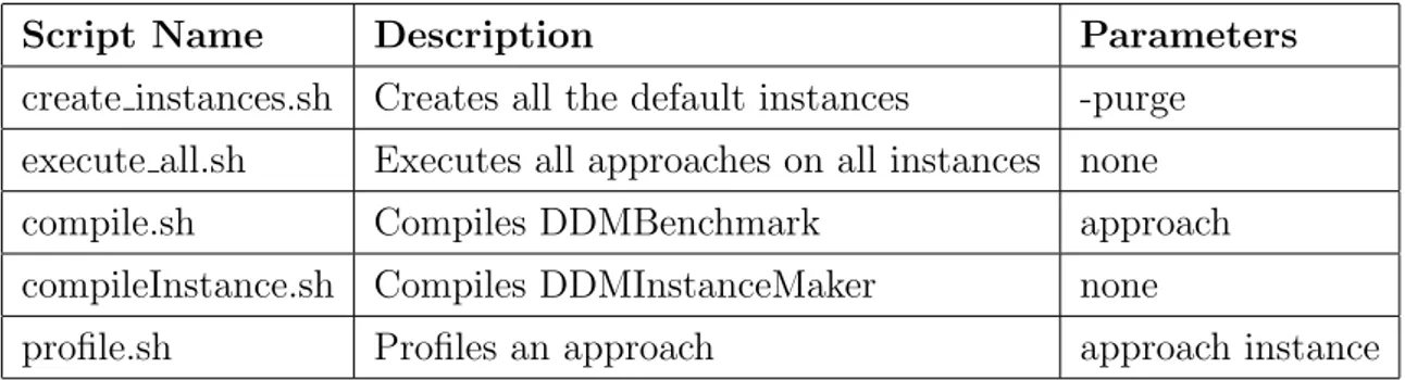
DDMBenchmark comes with some useful scripts that can help you to execute your code more easily. They are shown in table 3.4.4.
It is possible to compile the testbed using the provided compile.sh shell script3 placed in the root folder, and passing to it as the first parameter the
exact same name that has been given to folder that contains the Algorithm.c file. If the compilation succeeds it will be possible to try solving a certain instance running the command:
1 . / DDMBenchmark − i <instanceName>
Script Name Description Parameters create instances.sh Creates all the default instances -purge
execute all.sh Executes all approaches on all instances none compile.sh Compiles DDMBenchmark approach compileInstance.sh Compiles DDMInstanceMaker none
profile.sh Profiles an approach approach instance Table 3.3: Scripts
3.5
Summary
In this chapter we described how the testbed is structured and how its main components work.
We have seen that the testbed is divided in two main components, DDMIn-stanceMaker and DDMBenchmark. The first handles the generation of in-stances with a user provided set of parameters, while the second executes a proposed approach, checks for the validity of the solution and than rates the goodness of the approach using three criteria.
Then we described the evaluation criteria that have been taken into ac-count by our tested (that is distance from optimal solution, execution time and memory occupied), and we show how we compute a representative score. Moreover we discussed how we coped with some issues such as data over-flows and a realistic multi-step instance generation. Then we provided all the useful information to implement a new approach and run it under our DDMBenchmark’s control.
Now we’re ready to create the set of peculiar instances described in table 3.1 on page 20 and to implement some resolution approaches using some of the algorithm we described in chapter 2.
The results we got from our test implementations are shown and discussed in the following chapter.
Implementation Results
After we finished coding the testbed we were looking forward to test it with different kinds of approaches. We implemented three different region-based approaches, the most important ones, and a static grid-region-based one, described in chapter 1. Their commented code can be found within the Algorithms folder.
Firstly we implemented the Brute Force (described in section 2.2.1.1 on page 8), as we use it to solve our instances in DDMInstanceMaker. As we’ll see, it is quite efficient as it doesn’t use any additional data structures to perform the matching, and thanks to a short circuit logic it can avoid some of the overlapping checks.
The second algorithm that we implemented was the sort based (see sec-tion 2.2.1.2 on page 8). It is based on a previous work made by another student,[14] but we adapted it to make it work with our benchmark.
It was implemented in a very efficient way: as the sort based algorithm uses lists of a well known size, it is possible to use bitvectors (that are single lines of a bitmatrix) to store these “lists”, other than dynamically allocate each element. In this way all the operations are executed on a bit level, that are the most efficient, and they don’t require system calls on each insertion. The third one was the static grid-based (see section 2.2.2.1 on page 13). We divide each dimension in PARTS cells (i.e. the total number of cells is
P ART Sdimensions). For efficiency purposes and ease of implementation, we
only support two dimensional instances. To support unlimited dimensions we should change a nested loop with recursive calls, losing in efficiency.
This is the only approach we implemented that is not optimal (see section 1.2 on page 3 to see what we mean for optimal ). For this reason, we have made 4 versions with 4 different values for PARTS (2, 10, 30, 50) to show how much the solution improves increasing the number of cells.
The last approach we implemented is one of the most recent in literature. It is the partition based approach (see section 2.2.1.3 on page 10). In some circumstances it can perform a lot of recursive calls. Moreover it uses dy-namically allocated lists as we have to directly access all the elements of the lists very frequently.
The following section contains the results we got running our algorithms on five representative instances: Sparse, Average, Big, Huger and Cluttered.
4.1
DDM Instances
4.2
Results
The results you are about to read in the next sections were obtained on a PC running Ubuntu 13.04 (x64). It has an Intel core i7 CPU 920R
(@2.67GHz x 8) and 6GB of RAM (5,8GB of which are addressable). The data is the result of an average of three executions ran from text mode.
In the following sections we are going to show a detailed view of the results we got. For each instance we will show a bar graph for the execution time, one for the memory peak and one for the final score they got. As three out of four algorithm are exact, we won’t show a comparison for the distance from the optimal solution for each of them, but we just compare the distance obtained running our four static grid-based approaches.
Sparse
Dimensions: 2
Subscribers’ extents: 1000 Publishers’ extents: 1000
As this instance has a very limited number of extents, and they have a very small size, grid-based approaches are the best choice, as in this case they provide a low distance even when the number of cells is limited. Brute force approach gets the best score overall, as it consumes less memory than the other approaches and provides an optimal solution. It has only been slightly beaten in execution time by the partition based approach, but not that much to justify it’s higher use of memory.
Execution Time 0 2 · 10−2 4 · 10−2 6 · 10−2 8 · 10−2 0.1 0.12 0.14 Grid2 Grid10 Grid30 Grid50 Brute Partition Sort 5.02 · 10−4 6.14 · 10−4 1.02 · 10−3 1.43 · 10−3 4.33 · 10−2 3.49 · 10−2 0.13 Execution Time (s)
Memory Peak 1.45 1.5 1.55 1.6 1.65 1.7 1.75 ·107 Grid2 Grid10 Grid30 Grid50 Brute Partition Sort 1.52 · 107 1.52 · 107 1.58 · 107 1.68 · 107 1.52 · 107 1.74 · 107 1.61 · 107 Memory Peak (B) Distance 0 0.1 0.2 0.3 0.4 0.5 0.6 Grid2 Grid10 Grid30 Grid50 0.25 1 · 10−2 1.11 · 10−3 4.14 · 10−4
Score 0 0.5 1 1.5 2 2.5 3 3.5 ·104 Grid2 Grid10 Grid30 Grid50 Brute Partition Sort 32,364 8,435 7,822 8,251 7,857 8,828 9,135 DDMBenchmark Score
Average
Dimensions: 2 Subscribers’ extents: 4000 Publishers’ extents: 3500As in the SPARSE instance, brute force remains the best choice only looking at the score, but sort based approach executes on average twenty milliseconds faster. As this instance has bigger extents than the Sparse one, the grid-based approaches get worse result because of the higher distance from the optimal solution.
Execution Time 0 5 · 10−2 0.1 0.15 0.2 0.25 0.3 0.35 Brute Grid10 Grid2 Grid30 Grid50 Partition Sort 0.27 8.55 · 10−3 1.66 · 10−3 5.31 · 10−2 0.14 0.35 0.25 Execution Time (s) Memory Peak 1.45 1.5 1.55 1.6 1.65 1.7 1.75 1.8 1.85 1.9 1.95 2 ·107 Brute Grid10 Grid2 Grid30 Grid50 Partition Sort 1.64 · 107 1.65 · 107 1.64 · 107 1.68 · 107 1.76 · 107 1.95 · 107 1.76 · 107 Memory Peak (B)
Distance 0 0.1 0.2 0.3 0.4 0.5 0.6 Grid2 Grid10 Grid30 Grid50 0.58 0.15 5.37 · 10−2 3.16 · 10−2
Relative distance from optimal solution Score 0 1 2 3 4 5 6 7 ·104 Brute Grid10 Grid2 Grid30 Grid50 Partition Sort 10,776 23,460 65,915 14,123 13,138 13,008 11,029 DDMBenchmark Score
Big
Dimensions: 2 Subscribers’ extents: 10000 Publishers’ extents: 11000As the size of the instance increases, sort based runs faster than brute force and gets the best score if we don’t consider grid-based approaches. Partition based dynamic allocation starts to be evident looking at its execution time. Between the grid-based approach, Grid30 was the best compromise between the correctness of the result and the memory and execution time taken. Execution Time 0 0.5 1 1.5 2 2.5 3 3.5 4 Brute Grid10 Grid2 Grid30 Grid50 Partition Sort 2.18 6.15 · 10−2 1.4 · 10−2 0.38 1 4.08 1.92 Execution Time (s) Memory Peak 1.5 2 2.5 3 3.5 4 4.5 5 ·107 Brute Grid10 Grid2 Grid30 Grid50 Partition Sort 2.95 · 107 2.97 · 107 2.95 · 107 3.08 · 107 3.3 · 107 4.7 · 107 3.26 · 107 Memory Peak (B)
Distance 0 0.1 0.2 0.3 0.4 0.5 0.6 Grid10 Grid2 Grid30 Grid50 0.15 0.58 5.27 · 10−2 3.2 · 10−2
Relative distance from optimal solution Score 0 1 2 3 4 5 6 7 ·104 Brute Grid10 Grid2 Grid30 Grid50 Partition Sort 36,182 30,396 72,254 24,071 29,309 63,735 35,091 DDMBenchmark Score
Huger
Dimensions: 2 Subscribers’ extents: 20000 Publishers’ extents: 30000Partition based still gets a very bad score, due to its high use of resources (in time and memory). This is due to the fact that he consumes time dy-namically allocating memory, that is very onerous as implies system calls. As in the Big instance, sort based algorithm gets the best score (and we expect that it will decrease as the size of the instance grows).
Execution Time 0 5 10 15 20 25 30 35 Brute Grid10 Grid2 Grid30 Grid50 Partition Sort 12.07 0.32 6.07 · 10−2 1.95 5.16 33.86 10.4 Execution Time (s) Memory Peak 0.2 0.4 0.6 0.8 1 1.2 1.4 1.6 1.8 ·108 Brute Grid10 Grid2 Grid30 Grid50 Partition Sort 9.33 · 107 9.37 · 107 9.33 · 107 9.67 · 107 1.03 · 108 1.77 · 108 1 · 108 Memory Peak (B)
Distance 0 0.1 0.2 0.3 0.4 0.5 0.6 Grid10 Grid2 Grid30 Grid50 0.15 0.58 5.24 · 10−2 3.17 · 10−2
Relative distance from optimal solution Score 0 0.5 1 1.5 2 2.5 3 3.5 4 4.5 ·105 Brute Grid10 Grid2 Grid30 Grid50 Partition Sort 1.66 · 105 64,084 1.04 · 105 71,904 1.05 · 105 4.25 · 105 1.53 · 105 DDMBenchmark Score
Cluttered
Dimensions: 2 Subscribers’ extents: 50000 Publishers’ extents: 450001 t i m e s e c o n d s s e c o n d s c a l l s ms/ c a l l ms/ c a l l name 2 3 8 . 4 4 6 9 . 0 5 6 9 . 0 5 E x e c u t e A l g o r i t h m 3 3 1 . 6 7 1 2 5 . 9 4 5 6 . 8 9 41006 5408 0 . 0 0 0 . 0 0 i s S e t 4 2 3 . 3 6 1 6 7 . 9 0 4 1 . 9 5 4 5 0 0 0 0 0 0 0 0 0 . 0 0 0 . 0 0 r e s e t b i t m a t
Figure 4.1: The profiler revealed that these two functions took most part of the total execution time.
The CLUTTERED instance is the one that gives us the most interesting results. Its big and numerous extents gives us a lot to think about. Finally the partition based gets the best score with an extraordinary low execution time (only 1.13 seconds) that balances it’s use of the memory.
On the other hand, the sort based algorithm unexpectedly performs worse than the Brute force. This is a clear symptom that something is not working as it should. We profiled our sort based code using the profile.sh script (that runs GNU gprof profiler tool), and we found out that our bit level implementation is inefficient, but luckily it can be easily improved.
This was how the first version was implemented: 1 f o r ( j = 0 ; j <s u b s c r i p t i o n s ; j ++) 2 { 3 i f ( i s S e t ( S b e f o r e , j ) ) // Checks i f t h e b i t i n t h e p o s i t i o n j o f t h e b i t v e c t o r i s s e t 4 { 5 // R e s e t t h e p o s i t i o n j o f t h e b i t v e c t o r t h a t c o r r e s p o n d t o t h e update i d i n t h e r e s u l t b i t m a t r i x .
6 r e s e t b i t m a t ( ∗ m a t c h i n g r e s u l t , /∗ update i d ∗ / , j /∗ i . e . s u b s c r . i d ∗ / ) ;
7 } 8 }
That can be improved in:
1 // Negate t h e S b e f o r e b i t v e c t o r , a s we have t o r e s e t a l l t h e b i t s t h a t a r e s e t i n S b e f o r e
2 n e g a t e v e c t o r ( S b e f o r e , s u b s c r i p t i o n s ) ;
3 // Perform an AND between t h e /∗ update i d ∗/ row o f t h e r e s u l t b i t m a t r i x and t h e S b e f o r e v e c t o r . 4 v e c t o r b i t w i s e a n d ( m a t c h i n g r e s u l t [ / ∗ Update i d ∗ / ] , S b e f o r e ) ; 5 // Negate t h e S b e f o r e v e c t o r a g a i n t o b r i n g i t back t o i t s o r i g i n a l s t a t e ( t h i s a v o i d s c r e a t i n g a n o t h e r temp v e c t o r ) 6 n e g a t e v e c t o r ( S b e f o r e , s u b s c r i p t i o n s ) ;
As this piece of code was the core part of sort based, this small change caused a huge improvement in the execution time on bigger instances. To be coherent with the previous data, in the following graphics we continue to report the standard sort based, in the next section you can see how much the second sort based is faster.
Execution Time 0 10 20 30 40 50 60 Brute Grid10 Grid2 Grid30 Grid50 Partition Sort 22.46 0.15 0.14 0.17 0.17 1.13 55.61 Execution Time (s) Memory Peak 1 2 3 4 5 6 ·108 Brute Grid10 Grid2 Grid30 Grid50 Partition Sort 3.04 · 108 3.04 · 108 3.04 · 108 3.09 · 108 3.18 · 108 6.11 · 108 3.17 · 108 Memory Peak (B)
Distance 0 0.1 0.2 0.3 0.4 0.5 0.6 Grid10 Grid2 Grid30 Grid50 9.99 · 10−3 0.25 1.11 · 10−3 4 · 10−4
Relative distance from optimal solution Score 0 1 2 3 4 5 6 7 ·105 Brute Grid10 Grid2 Grid30 Grid50 Partition Sort 3.73 · 105 1.51 · 105 1.75 · 105 1.53 · 105 1.57 · 105 3.1 · 105 7.11 · 105 DDMBenchmark Score
4.3
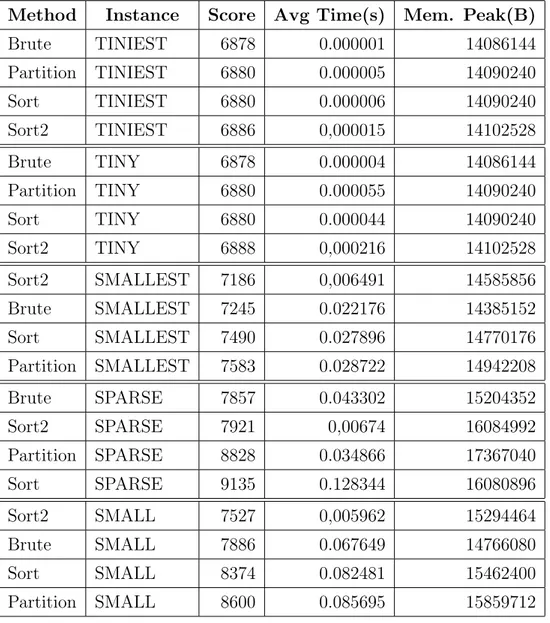
Tables
In this section we include, for completeness, the results we got from the execution of all the single-step instances in a tabular view. As you can see, in bigger instances (starting from SMALLEST, except from SPARSE) sort based 2 is the best choice.
Method Instance Score Avg Time(s) Mem. Peak(B) Brute TINIEST 6878 0.000001 14086144 Partition TINIEST 6880 0.000005 14090240 Sort TINIEST 6880 0.000006 14090240 Sort2 TINIEST 6886 0,000015 14102528 Brute TINY 6878 0.000004 14086144 Partition TINY 6880 0.000055 14090240 Sort TINY 6880 0.000044 14090240 Sort2 TINY 6888 0,000216 14102528 Sort2 SMALLEST 7186 0,006491 14585856 Brute SMALLEST 7245 0.022176 14385152 Sort SMALLEST 7490 0.027896 14770176 Partition SMALLEST 7583 0.028722 14942208 Brute SPARSE 7857 0.043302 15204352 Sort2 SPARSE 7921 0,00674 16084992 Partition SPARSE 8828 0.034866 17367040 Sort SPARSE 9135 0.128344 16080896 Sort2 SMALL 7527 0,005962 15294464 Brute SMALL 7886 0.067649 14766080 Sort SMALL 8374 0.082481 15462400 Partition SMALL 8600 0.085695 15859712
Method Instance Score Avg Time(s) Mem. Peak(B) Sort2 AVERAGE 8707 0,012995 17567744 Brute AVERAGE 10770 0.273851 16449536 Sort AVERAGE 11029 0.245308 17563648 Partition AVERAGE 13008 0.348612 19501056 Sort2 MEDIUM 10165 0,022593 20357120 Brute MEDIUM 15063 0.591967 18726912 Sort MEDIUM 15173 0.523543 20353024 Partition MEDIUM 20693 0.879791 24363008 Sort2 GRANDE 14000 0,04906 27668480 Sort GRANDE 26801 1.329336 27664384 Brute GRANDE 27385 1.514798 25063424 Partition GRANDE 44707 2.631536 37666816 Sort2 BIG 16613 0,067118 32649216 Sort BIG 35091 1.915111 32645120 Brute BIG 36162 2.174285 29532160 Partition BIG 63735 4.076749 47038464 Sort2 HUGE 24641 0,11618 48087040 Sort HUGE 61308 3.783034 48082944 Brute HUGE 64568 4.32241 43712512 Partition HUGE 145863 10.866742 76177408 Sort2 HUGER 51606 0,253202 100503552 Sort HUGER 153056 10.398484 100499456 Brute HUGER 166428 12.087455 93294592 Partition HUGER 425050 33.86481 176951296 Sort2 CLUTTERED 162445 0,746714 317394944 Partition CLUTTERED 309659 1.13438 610951168 Brute CLUTTERED 368221 21.993312 303693824 Sort CLUTTERED 711100 55.612473 317390848