POLITECNICO DI MILANO
Scuola di Ingegneria Industriale e dell’Informazione
Corso di Laurea Magistrale in
Mechanical Engineering
A MODELLING APPROACH TO ESTIMATE
THE IMPACT OF PALLETS WITH ZERO
POINTS CLAMPING IN A FMS
Relatore: prof. Marcello URGO
Correlatore: ing. Walter TERKAJ
Tesi di Laurea di:
Giorgio Luigi MOTTA Matr. 836888
Index
Table of Figures ... IV Table of Tables ... V Table of Graphs ... VII Table of Equations ... VIII Abstract ... IX Sommario ... XI Ampio estratto in lingua italiana ... XIII
1 Introduction ... 1
1.1 Flexible Manufacturing System ...1
1.1.1 Types of FMS ...3
1.2 Reconfigurable Pallet ...4
1.3 Problem Statement ...6
1.4 System Modeling ...7
2 FMS Model ... 11
2.1 FMS Features and Modeling ...11
2.1 Model definition ...13
2.2 Model choice ...14
3 Model Description ... 21
3.1 Introduction ...21
3.2 Algorithm procedure ...21
3.3 Features of the FMS modeled ...22
3.4 Queuing Networks model ...24
3.5 Features and constraints of the algorithm ...27
3.5.1 Events classification ...27
3.5.2 Classification of periods ...28
4 Transition analysis ... 29
4.1 Introduction ...29
5.1 Java Modelling Tools ... 41
5.2 Integration of algorithm and JMT ... 43
5.3 Simulated time and results acquisition ... 44
5.4 Positions of Jobs in the system ... 49
6 Validation of the model ... 53
6.1 KPI (Key Performance Indicators) ... 53
6.1.1 Throughput and Time Elapsed ... 53
6.1.2 Utilization ... 54
6.1.3 PUT (Pallets Unused over Time) ... 55
6.2 Validation Experiments ... 56
6.2.1 Single pallet validation ... 59
6.2.2 Multiple pallets of the same class ... 64
6.2.3 Multiple states with single classes ... 66
6.2.4 Multiple states with multiple classes ... 68
6.3 Conclusion ... 70 7 Performance Evaluation ... 71 7.1 Introduction ... 71 7.2 Performance comparison... 71 7.2.1 Factorial Experiment ... 74 7.2.2 Factors Description ... 76 7.2.3 Performance Indicators ... 77
7.2.4 Experiments Results (Exploitation Factor) ... 79
7.2.5 Experiments Results (Adjusted Throughput) ... 88
III
7.3.2 Performance Comparison ...99
7.3.3 Comparison of costs of different production strategies ...101
7.3.4 Conclusion ...109
Conclusion ... 111
Appendix ... 113
storage unit... 3
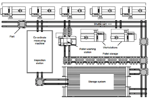
Figure 1.3 Flexible manufacturing cell with three identical processing stations, a load/unload station, and parts handling system ... 4
Figure 1.4 Tombstone with calibrated holes... 5
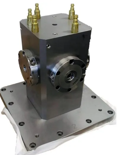
Figure 1.5 Zero point clamp ... 5
Figure 1.6 Tombstone with zero point clamps ... 6
Figure 2.1 Graphical representation of a station in Queueing Theory ... 14
Figure 3.1 Example of succession of periods ... 22
Figure 3.2 Queueing Networks model for FMS (1) ... 24
Figure 3.3 Queuing Networks model for FMS (2) ... 25
Figure 3.4 Blocks’ description of type of events ... 27
Figure 4.1 Graph of transitions between two states ... 31
Figure 4.2 Graph of transitions between two states: compatible transitions (B completed) ... 33
Figure 4.3 Graph of transitions between two states: compatible transitions (A completed) ... 34
Figure 4.4 Transitions tree of a simple system ... 36
Figure 4.5 Evolutions of transitions tree to a Ghost State ... 37
Figure 5.1 Graph of Queueing Network Model used in Java Modelling Tools . 42 Figure 5.2 Logger positions in the model ... 50
V
Table of Tables
Table 2.1 Short description of methods to solve Queueing Networks with
Blocking ...18
Table 2.2 Review of methods to solve Queueing Networks with Blocking ...18
Table 3.1 Description of different kinds of periods ...28
Table 4.1 Sequence of states ...30
Table 4.2 Description of state 1 (Table 4.1) ...30
Table 4.3 Boolean Possibility Matrix ...32
Table 4.4 Fluctuating Demand ...38
Table 5.1 Example of Log file ...44
Table 5.2 Example of Log file for system Throughput of Class 1 ...46
Table 5.3 Example of Log file for system Throughput of Class 2 ...46
Table 5.4 Example of input Log file ...51
Table 5.5 Example of output Log file ...51
Table 6.1 Service Times of Classes in each Station [minutes] ...56
Table 6.2 Probabilistic Routing Matrix (Class 1) ...57
Table 6.3 Probabilistic Routing Matrix (Class 2) ...57
Table 6.4 Probabilistic Routing Matrix (Class 3) ...58
Table 6.5 Demand of each Class ...58
Table 6.6 Capacity of Queues ...58
Table 6.7 Possibility Matrix ...59
Table 6.8 Throughput and Time Elapsed over runs (Single pallet) ...60
Table 6.9 Utilization of Machines (Single Pallet) ...61
Table 6.10 Mean Statistical Value of Throughput and Utilization (Single Pallet) ...62
Table 6.11 Mean Statistical Values (Multiple Pallets) ...64
Table 6.12 States compositions (Multiple states with single classes) ...66
Table 6.13 Pallets Unused over Time (Multiple States with single classes) ...66
Table 6.14 Throughput and Duration over periods (Multiple States with single classes) ...67
Table 6.15 Utilization of machines over periods (Multiple States with single classes) ...67
Table 6.16 States composition (Multiple States with multiple classes) ...68
Table 6.17 Pallets Unused Time (Multiple States with multiple classes) ...68
Table 6.18 Throughput and Duration over periods (Multiple States with multiple classes) ...69
Table 6.19 Utilization of machines (Multiple States with multiple classes) ...69
Table 7.6 2^k Factorial Plan ... 75
Table 7.7 Factors Levels (Factors NS - K - NC - RD - TREC) ... 76
Table 7.8 Factors Levels (Factor TMAC) ... 76
Table 7.9 Experiments Results (Exploitation Factor) ... 81
Table 7.10 Experiments Results (Adjusted Throughput) ... 88
Table 7.11 Experiments Results (PUT %) ... 93
Table 7.12 Couples of Performance Samples with 20 and 0 minutes of TREC (Adjusted Throughput) ... 100
Table 7.13 Extra Pallets percentages of replicates ... 102
Table 7.14 Descriptive Statistics of ΔK% ... 103
Table 7.15 Exact Probabilities for ΔMC values chosen ... 109
VII
Table of Graphs
Graph 5.1 Throughput plot for both classes ...48
Graph 5.2 Pieces-over-Time plot for both classes ...48
Graph 6.1 Throughput Plot ...61
Graph 6.2 Utilization Plot (Single Pallet) ...62
Graph 6.3 Throughput Plot (Multiple Pallets) ...64
Graph 6.4 Utilization of machines (Multiple pallets) ...65
Graph 7.1 Main Effects Plot (Exploitation Factor) ...82
Graph 7.2 Interaction Plot (Exploitation Factor) ...82
Graph 7.3 Main Effects Plot (Adjusted Throughput) ...89
Graph 7.4 Interactions Plot (Adjusted Throughput)...89
Graph 7.5 Approximated Model for Adjusted Throughput ...92
Graph 7.6 Main Effects Plot (PUT %) ...94
Graph 7.7 Interaction Plot (PUT %) ...94
Graph 7.8 Differential Cost ...104
Graph 7.9 Differential Cost Plot (ΔK% min = 0.66) ...105
Graph 7.10 Differential Cost Plot (ΔK% mean = 0.92) ...105
Graph 7.11 Differential Cost Plot (ΔK% max = 1.00) ...106
Graph 7.12 Region of Profitability of Zero Points Clamping ...107
Graph 7.13 Cumulative Probability Plot of ΔK% ...108
Graph 7.14 Probability that zero points are the best choice, in function of ΔMC ...109
Equation 6.1 Throughput ... 54
Equation 6.2 Utilization ... 54
Equation 6.3 Pallets Unused over Time ... 55
Equation 6.4 PUT Percentage ... 55
Equation 6.5 Expected Cycle Time ... 63
Equation 7.1 Reference Machining Rate (RMR) ... 78
Equation 7.2 Mean Machining Rate (MMR) ... 78
Equation 7.3 Adjusted Throughput (THadj) ... 78
Equation 7.4 Exploitation Factor (EF)... 79
Equation 7.5 Approximated Model for Adjusted Throughput ... 91
Equation 7.6 System of Equations for Cost Analysis ... 102
IX
Abstract
This thesis is mainly concerned with assessment of benefits brought by the employment of a new innovative type of pallet for Flexible Manufacturing Systems. This pallet is characterized by peculiar clamps, called zero points, able to decrease considerably the time needed for reconfiguration of the pallet itself. This analysis could be useful for those companies interested in investing in this type of production system.
The main aspect of the thesis is the evaluation of performances of the FMS applying these modern pallets. A tool done for this purpose has been built: it divides the whole production campaign in periods, using an algorithm. A simulation software evaluates performances of each period. The algorithm is implemented in MATLAB software, while the simulation is conducted by Java Modelling Tools, a software developed by Politecnico di Milano.
Several evaluations have been conducted to compare performances achieved using zero points with standard pallets’ ones. The comparison is realized with a statistical analysis, the ANOVA test. It is demonstrated that performances are better when the FMS works with modern pallets. A linear model is built to describe the increment of throughput in function of the reconfiguration time. Then the thesis concerns an additional performance comparison between throughputs achieved with zero points clamps and the highest ones reachable with standard pallets. This comparison proves that there are no differences in throughputs. The research ends with an economic analysis demonstrating that modern pallets are preferable in many cases.
Key words: Flexible Manufacturing System, performance evaluation, pallet, zero points
XI
Sommario
Questa tesi riguarda principalmente la valutazione dell’impatto di un nuovo innovativo tipo di pallet sulle prestazioni dei sistemi di produzione flessibili (Flexible Manufacturing Systems). Questo pallet è caratterizzato da prese particolari, chiamate zero points, in grado di ridurre notevolmente il tempo necessario per la riconfigurazione del pallet stesso. Questa analisi potrebbe essere utile ad aziende interessate ad investire in questo tipo di sistema di produzione. L'aspetto principale della ricerca è la valutazione delle prestazioni del sistema di produzione FMS al fine di stimare i possibili benefici portati dai moderni pallet. È stato appositamente costruito uno strumento di modellazione: esso suddivide la campagna di produzione in periodi, tramite un algoritmo. Per ogni periodo viene condotta una valutazione delle prestazioni tramite un software di simulazione. L'algoritmo è implementato nel software MATLAB, mentre la simulazione è condotta da Java Modelling Tools, un software sviluppato dal Politecnico di Milano.
Sono stati effettuati diversi esperimenti per confrontare le prestazioni ottenute con gli zero points con quelle ottenute con i pallet standard. Il confronto è stato realizzato con un’analisi statistica, il test ANOVA. É stato, quindi, dimostrato che le prestazioni sono migliori quando il sistema lavora con pallet moderni. In seguito è stato costruito un modello lineare per descrivere l’incremento della velocità di produzione in funzione del tempo di riconfigurazione.
La tesi si conclude con un confronto delle velocità di produzione ottenute con gli zero points rispetto alle massime raggiungibili con pallet standard. Questo confronto dimostra che non ci sono differenze di velocità. Infine è stata condotta un'analisi economica che dimostra che i pallet moderni sono preferibili in molti casi realistici.
Parole chiave: Flexible Manufacturing System, valutazione delle prestazioni, pallet, zero points
XIII
Ampio estratto in lingua italiana
La tesi riguarda la valutazione delle prestazioni di un sistema FMS, al fine di stimare i possibili benefici portati dall’utilizzo di un pallet di nuova generazione. Un FMS è un sistema di produzione basato su macchine utensili automatizzate, collegate tra loro da un trasportatore. I pallet sono le strutture che vengono movimentate tra le stazioni, sulla quale sono supportati i pezzi da lavorare tramite determinati agganci e prese. Il progetto mira a valutare l’effetto dell’utilizzo di particolari prese, chiamate zero points: esse permettono di riconfigurare il pallet, quindi modificarne il setup per sostenere parti diverse, molto più velocemente rispetto ai pallet standard.
Per la valutazione delle performance è necessario un modello in grado di riprodurre l’andamento della produzione nel FMS e la riconfigurazione dei pallet. Un metodo ampiamente utilizzato per la valutazione di sistemi di questo tipo è il modello a reti di code (Queueing Networks): è un modello analitico basato su stazioni interconnesse tra loro, ognuna composta da uno o più serventi e da una coda. Sono stati analizzati diversi modelli di Queueing Networks al fine di selezionarne uno aderente al sistema in questione: le caratteristiche principali richieste sono la presenza di blocking (code a capacità finita) e la possibilità di riconfigurazione. Mentre il blocking è presente in diversi modelli, la riconfigurazione dei “clienti”, cioè la modifica delle loro caratteristiche, è attuabile solo con un metodo probabilistico, che non rispecchia il vero andamento di un FMS.
La riconfigurazione dei pallet è stata valutata tramite un particolare algoritmo sviluppato in ambiente MATLAB. Esso divide la campagna di produzione in periodi, ognuno dei quali riproduce la lavorazione di una particolare composizione di pallet nel sistema. Le diverse configurazioni dei pallet sono chiamate “classi” ed ognuna di esse ha una richiesta di produzione. L’algoritmo valuta la composizione e la durata dei periodi basandosi sui risultati delle valutazioni delle prestazioni effettuate sui singoli periodi: ogni periodo finisce quando la domanda di una classe di pallet è stata soddisfatta. I pallet terminati vengono quindi riconfigurati, i rimanenti continuano la produzione fino al loro reinserimento nel sistema. Un esempio è visibile in Figura 1: ogni riga corrisponde a un pallet ed ogni lettera ad una classe. La timeline scandisce il tipo di periodi: semplice (S), cioè di durata variabile in base alla richiesta di produzione, e di riconfigurazione (R), cioè di durata fissata pari al tempo di riconfigurazione dei pallet estratti dal sistema precedentemente.
Figura 1 Esempio di successione dei periodi produttivi
La campagna di produzione è stabilita da una successione di stati predefiniti: ognuno rappresenta un periodo con una particolare composizione di classi di pallet attraverso il quale il sistema deve obbligatoriamente passare. L’algoritmo determina le riconfigurazioni in base a questo input.
La valutazione delle prestazioni dei singoli periodi non può essere effettuata con metodi analitici, in quanto essi calcolano le performance del sistema a regime. La condizione di regime non è verificabile per i singoli periodi, data la loro durata variabile. Per questo motivo è stato adottato Java Modelling Tools, un software di simulazione basato sulle reti di code, opportunamente integrato con MATLAB, in grado di valutare le prestazioni del sistema ad un tempo definito.
Lo strumento di valutazione delle prestazioni è, quindi, composto da un algoritmo per dividere la produzione in periodi e da un software di simulazione per valutare le performance dei singoli periodi. È stato validato tramite casi semplici per verificare l’affidabilità dei risultati.
È stata progettata ed effettuata una campagna sperimentale utilizzando lo strumento costruito: essa è atta a valutare l’eventuale impatto dei pallet di nuova generazione sul sistema. La caratteristica che distingue i pallet moderni è il tempo di riconfigurazione: è stato fissato a 20 minuti, rispetto alle due ore dei pallet standard. Il piano sperimentale scelto è fattoriale di tipo 2^k: sono stati selezionati sei fattori, tra cui il tempo di riconfigurazione, ognuno con due livelli. Per ogni combinazione dei livelli dei fattori sono state valutate le prestazioni di tre diverse campagne di produzione (casi) generate casualmente. L’obiettivo è stimare l’effetto dei fattori sulle prestazioni del sistema, in particolare quello dato dal fattore tempo di riconfigurazione.
XV
adottati sono l’Exploitation Factor (EF), che valuta la frazione di tempo impiegato per la lavorazione dei pezzi rispetto al tempo totale, e l’Adjusted Throughput (THadj), cioè la velocità di produzione del sistema adattata rispetto ai tempi di lavorazione delle macchine utensili.
La prima analisi è stata effettuata utilizzando l’Exploitation Factor. Alcuni effetti sono risultati significativi: i principali sono il numero di pallet nel sistema, il tempo di riconfigurazione e il tempo di lavorazione delle macchine utensili. Le prestazioni migliorano quando aumenta il numero dei pallet od il tempo di lavorazione oppure quando diminuisce il tempo di riconfigurazione. Da un’analisi dell’interazione tra tempo di lavorazione e tempo di riconfigurazione si è scoperto che l’effetto di quest’ultimo è significativo solo per valori bassi del tempo di lavorazione. Per questo motivo, è stata effettuata un ulteriore studio dei dati. La seconda analisi è stata effettuata con l’indicatore THadj. L’ANOVA test è stato svolto su 5 fattori, eliminando il tempo di lavorazione ed utilizzando solo gli esperimenti con il livello più basso di questo fattore. Gli effetti significativi principali sono il numero di pallet ed il tempo di riconfigurazione, confermando i risultati dello studio precedente. L’analisi dimostra che i pallet di nuova generazione migliorano le prestazioni del sistema FMS: è possibile affermare che il loro utilizzo aumenta in media la velocità di produzione dell’8 %. Utilizzando i dati, è stato costruito un modello lineare approssimato che descrive l’andamento dell’Adjusted Throughput in funzione del numero di pallet e dei minuti risparmiati sul tempo di riconfigurazione. Il suo piano è visibile sul Grafico 1.
La tesi si conclude con un’analisi economica relativa all’utilizzo dei pallet con prese “zero points” rispetto a quelli standard. Le prestazioni ottenute da questi ultimi vengono massimizzate tramite una nuova strategia di produzione: essa prevede un tempo di riconfigurazione pari a zero raggiungibile tramite l’acquisto di un numero maggiore di pallet. Le performance raggiungibili con questa nuova strategia sono state confrontate con quelle dei pallet di nuova generazione con un Paired T-test. Il risultato del test dimostra che non ci sono differenze tra le velocità di produzione. L’analisi economica verte, quindi, sul confronto tra i costi prodotti dai pallet standard aggiuntivi richiesti e quelli dati dal prezzo d’acquisto maggiore dei pallet moderni. Tramite i dati degli esperimenti e un’analisi degli andamenti dei costi, è stato possibile sviluppare un modello che descrive la probabilità che i pallet di nuova generazione siano la scelta più redditizia. Esso è costruito in funzione dell’aumento percentuale di prezzo dei pallet moderni rispetto a quelli standard (ΔMC). La curva descritta dal modello è visibile sul Grafico 2. Si nota che per ΔMC minori di 0.75, la probabilità che i pallet con prese “zero points” siano la scelta migliore è maggiore del 90 %.
Grafico 2 Probabilità che i pallet moderni siano la scelta ragionevole, in funzione di ΔMC
È stato dimostrato, quindi, che i pallet di nuova generazione non solo aumentano le prestazioni del sistema FMS ma spesso sono anche economicamente vantaggiosi.
1 Introduction
The object of this thesis is the evaluation of performances of a generic Flexible Manufacturing System and the analysis of the possible improvements brought by the employment of a new kind of pallet.
The main goals are the analysis of the performance of the production program in terms of time elapsed, optimization in utilization of machines and throughputs achieved and the numeric and economic estimation of improvements of the new pallet compared with the utilization of a standard pallet.
1.1 Flexible Manufacturing System
A Flexible Manufacturing System is a composition of different service stations, each one with a different function such as machining, loading/unloading, quality check, connected by a generic vector: its common scope is machining parts that entered in the system. This kind of production system is widely used thanks to its high flexibility that provides capability to manage together a good variety of parts. The idea of an FMS was proposed in England (1960s) under the name "System 24", a flexible machining system that could operate without human operators 24 hours a day under computer control. From the beginning the emphasis was on automation rather than the "reorganization of workflow".
“An FMS consists of a group of processing work stations interconnected by means of an automated material handling and storage system and controlled by integrated computer control system” [1]. A simple scheme of a generic FMS is shown in Figure 1.1.
As already said, at start the idea of FMS was only strictly linked to the one of automation, but after some time the concept of flexibility rose and became more important. Recently, many new manufacturing facilities have been labelled FMS. This has caused some confusion about what constitutes an FMS. Flexibility and automation are the key conceptual requirements. However, it is the extent of automation and the diversity of the parts that are important; some systems are termed FMS just because they contain automated material handling. For example, dedicated, fixed, transfer lines or systems containing only automated storage and retrieval are not FMSs. Other systems only contain several (unintegrated) NC or CNC machines. Still other systems use a computer to control the machines, but often require long set-ups or have no automated parts transfer. The key feature to identify an FMS are automation and flexibility, but it is the definition of that last concept that is not so easy to face. It is an idea that can be linked to multiple situations and sectors. To help clarify the situation, eight types of flexibilities have been defined and described by Browne,Dubois,Rathmill,Sethi and Stecke [1]. Machine Flexibility: the ease of making the changes required to produce a
given set of part types.
Process Flexibility: the ability to produce a given set of part types, each possibly using different materials, in several ways.
Product Flexibility: the ability to changeover to produce a new (set of) product(s) very economically and quickly.
Routing Flexibility: the ability to handle breakdowns and to continue producing the given set of part types.
Volume Flexibility: the ability to operate an FMS profitably at different production volumes.
Expansion Flexibility: the capability of building a system and expanding it as needed, easily and modularly.
Operation Flexibility: the ability to interchange the ordering of several operations for each part type.
Production Flexibility: the universe of part types that the FMS can produce.
Introduction
3
1.1.1 Types of FMS
Flexible Manufacturing Systems are different one from each other because of shape, machines used, handling system, pallets, control system but they can be classified approximately basing on size and productive capability. Three types have been recognized: single machine cell, flexible manufacturing cell and flexible manufacturing system.
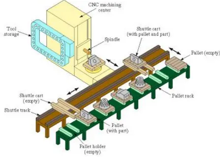
Single machine cell: it contains one machine (often a CNC machining center) connected to a parts storage system, which can load and unload parts to and from the storage system. It is designed to operate in batch mode, flexible mode, or a combination of the two. An example is shown in Figure 1.2.
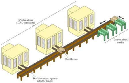
Flexible manufacturing cell: it contains two or three processing workstations (often CNC machining or turning centers), plus a parts handling system. This set-up can operate in flexible mode and batch mode, as necessary, and can readily adapt to evolving production schedule and increased production volumes. Figure 1.3 describes a possible flexible manufacturing cell.
Flexible manufacturing system: consists of four or more processing stations connected mechanically by a common parts handling system and electronically by a distributed computer system. FMS is larger than the flexible manufacturing cell, not only in the number of workstations it may contain, but also in the number of supporting stations in the system, such as part/pallet washing stations, co-ordinate measuring machines, storage stations and so on. Computer control is also more sophisticated; it includes functions not found in the flexible manufacturing cell such as diagnostics and tool monitoring.
1.2 Reconfigurable Pallet
Pallets and baseplates are main actors of a Flexible Manufacturing Systems together with machines. They are responsible for holding pieces and parts perfectly to let them be machined accurately. There are different types of pallets, everyone is studied for a specific group of parts and to be adaptable to a certain genre of machining centers. Baseplates are those metal panels, mounted on pallets, that physically support pieces. The most used pallet shape is the so-called
tombstone: a sort of turret where baseplates can be fixed on each side. An example
of that type can be seen on Figure 1.4.
Figure 1.3 Flexible manufacturing cell with three identical processing stations, a load/unload station, and parts handling system
Introduction
5
The thesis focuses on the utilization of a new tombstone pallet. This pallet is not a specific one, so designed and configured to accept only a certain family of parts or at least to be reconfigured in a long time, but it has been conceived to be reconfigurable in a short time. Different types of baseplates can be mounted on it to achieve setup desired quickly and when it's needed it can be reconfigured with new baseplates and so new part types. This quick setup is made possible by the presence of zero points clamps on tombstone’s surfaces. These kinds of clamps can fix and align baseplates in a perfect way without long mechanical actions or additional checks. This clamp is simply based on hydraulic or pneumatic system to fasten the baseplate with great accuracy. An example of a zero point clamp is visible in Figure 1.5, while a tombstone with them on is shown in Figure 1.6.
Figure 1.4 Tombstone with calibrated holes
The principal aim is to evaluate the gain obtained by the application of this new type of tombstone in terms of time and productivity against its cost, which it is higher than simple pallet’s one.
1.3 Problem Statement
The main issue of this thesis is the performance evaluation of a productive system with reconfigurations of clients. It means that features of pallets are not fixed all
Introduction
7
The first problem is the numeric evaluation of the progress of one or more pallets among stations of the FMS. This aspect can be defined concretely by some performance indicators such as time elapsed into the system or parts’ throughput of the system. Estimation of these values is the critical aspect of the research. It must consider a lot of different aspects: service time, presence of buffers, transportation system, different kinds of stations and parts, human intervention, reliability of machines, scraps.
The second issue is the employment of the new futuristic pallet. As already said, this kind of pallet is not specific for some parts, but it can be configured to accept any kind of parts. This fact implies that pallets in the system can change their classes of parts and so their features when needed. This is the critical aspect of the introduction of this new pallet: the variability in time of its features.
Those two issues must be considered together with the inputs of the performance evaluation; these are the production program, which classes of parts must be produced and their sequence for machining, and the demand, how many parts must be produced for each class. Tools presented in this thesis will be capable to evaluate performances of a production program on a Flexible Manufacturing System.
1.4 System Modeling
The first problem concerns several aspects of the Flexible Manufacturing System. The easiest method to model the system and to evaluate its performances is considering it as a sequence of machining times, each one related to a station where pallets go through. This is clearly an extreme approximation that is never like the real system, because there are several critical aspects about this modeling procedure that should be taken into account.
The first issue is the distribution and features of machining times. This concept is strictly related to the one of human intervention: in an FMS, human role is limited to supervision and loading/unloading. For this reason, times have not a high variance, nevertheless they cannot be considered deterministic and fixed. Even automated machines can incur in some delays provoked by changing tools or whatever similar.
The transportation system cannot be neglected: time elapsed in moving pallets between stations in general is not so low. It is also variable, it depends on type of vector, distances between stations and loading/unloading method.
Another problem is the presence of buffers and so interactions between pallets: pallets can’t be considered as moving in a free system, they can incur in another pallet that occupies the station they need and so their progress delays. The presence of buffers is crucial to manage these situations, so the model must comprehend these features.
Last issues are easier to be governed. Reliability can be approximated to 1 because those types of machines are not often affected by failures, while scraps can be included in demands of parts, after an empirical evaluation of their percentage. A good solution to approximate the Flexible Manufacturing System in these constraints is the employment of Queueing Networks. It is an analytical method that reproduces behavior of clients moving in a network of stations; in every station, each client spends time for waiting, if there are some others clients already in the station, and for service. Results obtained from this type of method concern the steady state condition of the system. Transportation system can be easily approximated as a station: the duration of the travel between stations is emulated by service time. There are several models for Queueing Networks, each one with different peculiarities to be good for different situations; an analysis is done in Chapter 2.
Once chosen a good QN model, the thesis focuses on the next issue, linked to the new reconfigurable pallet. The main constraint introduced is the variability in time of features and data of pallets: this fact modifies completely every interaction between clients and stations of the model. The thesis must take in account that after a certain period, defined in general by demand fulfilling, pallets can be extracted from the system and reconfigured with other fixtures and parts, and so with other characteristics. Some Queueing Network models have the chance to introduce a variability of features of the jobs of the network, but they are not suitable for this research. Those models, indeed, can emulate the change of attributes of clients, but they are governed by a probabilistic law and so they may reproduce some situations of the system which never happen or maybe they could avoid some other ones that will always arise. In other terms, a probabilistic law is not appropriate to reproduce a reconfiguration which is ruled by time. In order to respect the reconfiguration constraint, the performance evaluation has been divided in different time periods, each one with a different configuration of jobs and so with a different calculation of results. The passage between a period and the next one is the result of a reconfiguration of one or more pallets.
This new attribute of the performance evaluation is a strong innovation: the estimation is not done once for each group, made by system, production program and demand, but there are several evaluations to be done for the same group.
Introduction
9
constraint. It is not possible to know a priori the duration of each period, except for some of them, and so it is not easy to guess if system can reach steady state during the period. The thesis needs an evaluation model that gives results obtained after a certain time, even if steady state has not been attained. A possible solution is a simulation model: it can check the trend and values of performance indicators along time and so it can provide results at the end of the period, whatever condition has been reached. The simulation model and software employed in this thesis is Java Modelling Tools (Chapter 5).
This research applies a simulation model, based on Queueing Networks, to evaluate performance of each group composed by FMS, production program and demand; every period, with its unique configuration, is simulated singularly, then results are combined to get an overall outcome.
2 FMS Model
2.1 FMS Features and Modeling
Performance evaluation of productive systems is one of the most critical topics of manufacturing engineering. Especially talking about FMS, it is complicated to manage this type of system because of the quantity of different parameters and features that it involves.
Grieco, Semeraro and Tollio [5] defined that these components can describe a Flexible Manufacturing System:
-Machines
-Transportation System -Control System
-Tools and tool handling system -Parts, pallets, and fixtures
Machines in the system strongly affects performance and functioning. The first FMSs were composed of different machines with different capabilities. Slowly, this diversity was reduced and now many FMSs have identical machines. New machining centers are more versatile and they can work on different part types using different tools. All the operations needed by a part can often be done by a single machine.
The main issue about machines regards setup. In some cases, machining centers are tuned in different ways to have better accuracy on some specific parts. Transportation system is always automated in a FMS. Depending on the type of pallet the system can have different kind of handling system. Modeling this part of the FMS mainly affects the time for handling pallets between stations.
Control System influences behavior of the manufacturing system. At present, the control system of most of the existing FMSs is based on a “supervisor” coordinating the behavior of the various devices (machines, transport system, etc.) and on a set of Computerized Numerical Controls (CNCs) and Programmable Logic Controllers (PLCs), each of which controls a specific device.
The main problem is the integration between software, often supplied by different companies, and hardware, but during last years a great development in terms of standardization of CNC has been made.
Other important issues regarding control system concern how CNC manages part programs and operations. It affects possibility to split part programs over multiple machines, to apply a variable sequence of operations or to define alternative activities for the same product part.
Tools management is a critical issue of Flexible Manufacturing Systems and it is often neglected during performance evaluation or loading decision phase. It's strictly related to its life and tools storing system. Every tool used by machines is worn after some usage and so it should be reconditioned or changed: the main problem is the forecast of the life of the tool. The recent evolution of machining operations has provoked an increased difficulty in this type of analysis, due to the higher cutting speed reached.
Since tools are quite expensive, it is very important to decide how many copies of the same tool the system needs. Furthermore, it is crucial to develop an adequate storage system on every machine and a handling system that brings tools from and to machining centers.
Parts, pallets, and fixtures are different levels of the object that is worked by FMS. Machining centers work on parts, which are hooked to fixtures that are clamped on the pallet. It is important to check how many and which fixtures our parts need. The main issue regards the choice of the “unit” of the model between them and its connection with the other levels in terms of compatibility and time.
FMS Model
13
2.1 Model definition
The most used model to evaluate performance of an FMS is the Queueing Networks.
Queueing Networks is an analytical model based on a group of queues, linked basing on customer routing. Balsamo gave this definition [3]: “Queueing Networks models a set of service centers representing the system resources that provide service to a collection of customers that represent the users”.
Every station is based on the Queuing Theory. Queueing theory is a set of tools to analyze systems where clients arrive at service centers. This theory was initiated by A.K. Erlang in 1908 to solve problems in the telecommunication field. Since then the theory was extended and applied to many different fields including production systems and logistic systems. This theory determines the interaction between customers and a simple system made by a queue and one or multiple server, considering stochasticity of activities' time. The user simply arrives at the station and waits for service in the queue.
A queue is composed by a certain number of servers and the place where clients wait for service. A station is completely specified when six features are defined: statistics of the stochastic arrival, statistics of the stochastic service process, number of servers, queue capacity, total number of clients and dispatching policy. Generally, the Kendall’s notation is applied to describe a queue quickly:
A/S/m/K/N/ω. A and S, respectively statistics of arrival and service, can have
those following values:
M Exponential distribution Er Erlang distribution D Deterministic distribution G General distribution
While m stays for number of servers and it can assume any value between 1 and +∞; the same behavior is assumed by K and N, which are respectively queue capacity and total number of clients in the station (+∞ is the standard value assumed if no amount is defined). The last value ω represents the dispatching policy and it can be designated by any discipline, such as FCFS or similar (FCFS is standard one if it’s not specified). A graphical representation of that kind of queue is shown in Figure 2.1.
Big development introduced by Queueing Networks is that it takes into consideration interactions between stations. It evaluates different parameters of steady state behavior of the model in an analytical way. We can have three different types of Queueing Networks: open, closed and mixed. Open model considers the arrival of jobs from outside of the network, closed one does not accept external arrivals or jobs leaving network, number of jobs is always constant. Mixed model is in the middle between open and closed one.
2.2 Model choice
A lot of different Queueing Networks models has been implemented over years, each one with dissimilar peculiarities. This thesis studied some of them to choose one suitable for this problem.
Jackson's Networks is the oldest and simplest model [6]. It can be used for open models and it is easy to be implemented due to the product-form solution. Product-form networks have a simple closed form of the stationary state probability distribution, which allow the definition of efficient algorithms to evaluate their performance.
FMS Model
15
The first limit could be easily bypassed by approximating different classes of customers into one average class.
This thesis discards this type of network, because an FMS is better to be modeled as a closed model: pallets never go out of the system.
Gordon-Newell's Theorem proposed a closed queueing networks with features very similar to Jackson's ones [7]. Its solution is the same of Jackson's open model removing unfeasible states through a normalization. This normalization is based on a convolution algorithm that could bring to a high computational effort, especially if jobs and stations are several.
Gordon-Newell's model has been widely used for performance evaluation of FMS, due to its simple implementation that suits perfectly a system with low quantity of stations and customers such as Flexible Manufacturing Systems. However, its results are always altered due to limitations. Exponential service times is a feature that can be accepted by our model, but infinite capacity servers are not compatible with an FMS system. Stations have not a storage area before them acting as a queue.
Another model taken into consideration is BCMP Networks (Baskett, Chandy, Muntz and Palacios [8]). This was an important evolution into queueing networks' world, because of its introduction of different types of stations. Jackson's and Gordon-Newell's consider always a FCFS policy (First Come First Served) on stations' queues, BCMP model analyses four types of stations instead. These are: -FCFS discipline where all customers have the same negative exponential service time distribution. (The service rate can be state dependent.)
-Processor sharing queues (Jobs in stations are served contemporarily) -Infinite server queues
-LCFS (Last Come First Served) with pre-emptive resume (work is not lost)
As for Jackson, also BCMP can be considered as a product-form network. It is suitable for open, closed or mixed models with multiple classes of customers and various service disciplines and service time distributions. Its resolution can be achieved as usual with a convolution algorithm, but in 1980 Lavenberg and Reiser [9] developed a new method called Mean Value Analysis (MVA) that avoids the direct evaluation of the normalization constant. This is a recursive computational algorithm based on a set of recurrence equations between average performance
measures. MVA is preferred when the quantity of entities in the system loads heavily computational effort of convolution algorithm.
Another feature of BCMP is the multi-class analysis. Using this type of networks different type of classes can be considered without averaging them into a mean one, but computational cost grows exponentially with number of classes.
Main limit of classic BCMP Theorem is the absence of blocking, as for precedent models. In the recent past several researchers have tried to develop new solutions for these types of networks including blocking evaluation. One of the first was Akyildiz in 1988 [10], he suggested an approximate method to reproduce blocking mechanism. It is based on the application of a non-blocking solution evaluated with a fictitious number of jobs, different from the real one. This quantity of jobs is the one that reproduces several possible states equal to the one of a blocked system, estimated with the real quantity of customers. It is a weak method due to the high level of approximation.
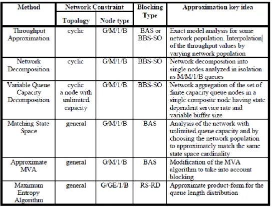
Blocking solutions implemented till now are founded on various methods such as recursive and convolution algorithms depending on type of network studied. Main exponent of this research field is Simonetta Balsamo, who implemented a good convolution algorithm in 1998 [11] suitable for all types of blocking mechanism. Then she collected and compared some blocking solutions for closed queueing networks [2000] [12] as can be seen in Table 2.1 and 2.2 (Tables taken from [12]). These algorithms are:
• Throughput Approximation (Onvural and Perros [13]) • Network Decomposition (Frein and Dallery [14])
• Variable Queue Capacity Decomposition (Suri and Diehl [15]) • Matching State Space (Akyildiz [10])
• Approximate MVA (Akyildiz [16])
• Maximum Entropy Algorithm (Kouvatsos and Xenios [17]).
The first three methods (Onvural and Perros, Frein and Dallery, Suri and Diehl) evaluate the throughput of cyclic networks with exponential service time distribution. The first and the third algorithm compute the throughput as a function of network population. The throughput approximation method applies to cyclic networks with BBS or BAS blocking. It assumes that the throughput is a symmetrical function of the population network. In the Frein and Dallery’s algorithm the throughput of the cyclic network with BBS blocking is
FMS Model
17
BBS blocking and where one node has infinite capacity (B1=¥). The algorithm is based on the network decomposition principle applied to nested subnetworks. The key idea is that given a node i, all the downstream nodes {i+1,…,M} are aggregated in a single composite node Ci+1 with load dependent service rate and a variable queue capacity.
Next three methods (both by Akyildiz, Kouvatsos and Xenios) apply to arbitrary topology networks. The first two methods assume BAS blocking and exponential service time and evaluate the network throughput. The third method assumes RS-RD blocking, generalized exponential service time, and it evaluates the queue length distribution and average performance indices.
The first Akyildiz method has been already explained in this chapter. The Approximate MVA by this author, instead, is different: Network with BAS blocking and exponential service times are analyzed with a modification of the MVA algorithm originally defined for product-form networks with unlimited queue capacities. The MVA algorithm is based in the Little theorem and the arrival theorem (Raiser and Lavenberg). Last method compared, the Maximum Entropy Algorithm, evaluates the queue length distribution and average performance indices of a network with RS-RD blocking and generalized exponential service time. The approximation is based on the principle of maximum entropy and is an extension of an algorithm defined for open networks. It has successively been extended to multiclass exponential networks.
Table 2.2 Review of methods to solve Queueing Networks with Blocking Table 2.1 Short description of methods to solve Queueing Networks with Blocking
FMS Model
19
There are three main blocking mechanism types:
-Blocking After Service (BAS): After a job completion at queue i, if the job attempts to enter to queue j which has reached the capacity constraint, then it is forced to wait at i (i.e. queue i is blocked). When a space becomes available at j, the job goes to queue j and service at queue i is resumed.
-Blocking Before Service (BBS): A job declares its destination queue j before it starts receiving service at queue i. If the job finds node j full, then queue i is blocked.
-Repetitive Service (RS): After a job completion at queue i, if the job attempts to enter to queue j which has reached the capacity constraint, then it starts a new and independent service at i (according to center i discipline).
FMS studied in this analysis can be reasonably modeled with a BAS blocking. In this manufacturing structure, jobs must wait for next machine availability before releasing the actual station. Some methods such as convolution algorithm developed by Balsamo or approximate MVA (Akyildiz) can be adequately used to model Flexible Manufacturing Systems.
Last issue of the system is the possible continuous reconfiguration. The new kind of pallet can be reconfigured as many times as the owner wants, so it is crucial to contemplate a continuous change of conditions into the system. This aspect implies that the performance evaluation cannot be always completed in steady-state conditions, as analytical methods concern, but an analysis of trend of parameters over time must be done. For this reason, the analysis has turned to a simulation model.
A discrete-event simulation approach has been chosen, based on Montecarlo Method, that reproduces stochastic events which happen in the Queueing Network system.
This procedure is well implemented in Java Modelling Tools (JMT). This is a software based on Java language for performance evaluation of any kind of systems using queueing models, born in Politecnico of Milan in collaboration with Imperial College of London [18].
The simulation section of this tool suits perfectly the FMS system, because it has several parameters that can be modified and adapted to situations. Moreover, it can achieve more accurate results.
It is also fundamental to consider a possible continuous change of classes into the system. This situation is accounted into BCMP networks and JMT simulation: it
is possible to study a probabilistic switching of classes. As already said a probabilistic approach does not suit the system in question, because it could reproduce some situations into the manufacturing system that are not possible in the real one.
Therefore, a simple performance evaluation system such as simulation or analytical method is not enough to properly study this procedure.
3 Model Description
3.1 Introduction
This research applies an algorithm that integrates simulation approach with reconfiguration issue. It recreates the production process of the FMS over time, taking into consideration reconfiguration events.
It receives demand and production program as inputs and it releases production performances of the system over time, such as throughput and utilization, and reconfiguration events as outputs. The main idea of the algorithm is splitting time in different periods; in each period a different configuration of the system is simulated.
The algorithm is responsible for periods sequence and succession, basing on analysis of simulation results of periods. It is the agent that links the simulation of a period with the next one. After an examination of performance values of the last simulated period, it generates duration of that period and configuration of the next one to be used as an input for simulation. Its main operations are the estimation of pallets to be extracted from the system: number and type of pallets to be inserted in the system, their composition, and positions of tombstones in the system.
3.2 Algorithm procedure
Sequence of period is defined by scheduling and reconfiguration events, which correspond to start and end of each period.
Periods can be distinguished into two categories: simple and reconfiguration.
Simple ones are those periods when FMS produces parts till fulfilling demand of
one of the pallets’ class. Their lengths are not fixed, but they depend on throughput performance simulated in each period.
Reconfiguration periods are fixed duration ones. They represent those periods in
which the system produces meanwhile reconfiguration takes part on some pallets. A peculiar reconfiguration period is the blank one: it is so called because no pallets are machined in the FMS.
These two types of periods are often alternated, except for periods when no new classes of pallets could be introduced or when a certain class finishes its production during a reconfiguration period. The example in Figure 3.1 demonstrates in a better way the succession of periods.
The example describes an FMS working with three pallets; each blue line in the figure represents one of them. The capital letter on the blue area defines the type (class) of the pallet during each period. Each class represents a certain configuration of baseplates, and so of parts, on a pallet. Orange area means that the pallet is subdued to reconfiguration outside the system.
Trend of different types of periods (‘S’ stands for Simple and ‘R’ for Reconfiguration) can be seen on the timeline.
This model divides evaluation in two activities: algorithm defines the succession of periods and simulation calculates performances in each period.
3.3 Features of the FMS modeled
This model can be adapted to different Flexible Manufacturing Systems, especially thanks to high flexibility of Java Modelling Tools. In this research a certain FMS model has been studied, with these characteristics:
-Machines: any quantity of machining centers can be considered. They are identical machines with different and variable setups, for this reason pallets cannot be sent to any machine but they have a peculiar route. Nonetheless
Model Description
23
-Transportation System: a simple automated carrier is considered. It can handle only one pallet per trip. Its time parameters are evaluated as weighted average values of different trips’ durations, depending on routing of each class and speed of the carrier.
-Control System: type and functioning of CNC are not important for performance evaluation, for this reason Control System is not contemplated into this analysis. -Tools and tool handling system: tool management has not been addressed in this model. Loss of time due to unavailability or change of tools can be approximated to a certain value to be added to processing times.
-Parts, pallets, and fixtures: the model assumes pallets as units of production of the manufacturing system. Each configuration of the pallet is defined as a class: all processing, routing and demand parameters change depending on class. Parts hooked to pallets are not accounted in this model. However, fixtures are a crucial part of the reconfiguration process. Different types of fixtures can be identified and each class of pallets has its own needed fixtures. This connection between pallets and fixtures is the main actor of the reconfiguration events that it is explained later.
-Storage and capacities: there are no external buffers in the system. All the stations of the model (carrier, machines, load/unload) have their own capacity; for this reason, the system can incur into blocking that has been determined as a BAS one. FCFS policy has been chosen for all queues.
3.4 Queuing Networks model
As already said, the FMS system can be modeled as a network of queues. There are two principal ways to model a Flexible Manufacturing System applying Queueing Networks. These two solutions have different features and approximations, but they are both good for FMS modeling.
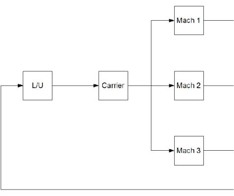
The first model is the one drawn in Figure 3.2.
The reference station is the Carrier, all the other queues are connected to it in the same way and their outputs become the input of the carrier, in order to close the network.
Model Description
25
The second solution for FMS modeling is shown in Figure 3.3.
In this case the reference station is the Load/Unload station: it is directly linked to the Carrier that brings the flow to Machines in the same way. Outputs of machines close the network returning to L/U queue.
These methods have different advantages and disadvantages. The second one is more affected by the route of the single pallet: it is loaded in the L/U station, then it is taken by the Carrier and brought to the Machines. There is no chance that the pallet doesn’t visit the Load/Unload station during each cycle; this fact makes the model more adherent to the real behavior of the system. The great approximation of this model is related to the Carrier: its station connects Load/Unload station to other machines but it doesn’t link the outputs of these machines to the input of L/U. This fact means that the model reproduces a behavior which is not possible in the real system: jobs are transported from machines to load/unload station without any carrier. The absence of the Carrier station after machines is compensated by the duplication of the service time of the Carrier. In this way, the service time of the Carrier simulates not only the travel between Load/Unload and the Machines, but also the inverse trip. Another lack of this model is associated
to number of machines needed by each job for machining: this model permits only one machine per pallet (without considering L/U).
The first model is more affected by the real composition of stations in the Flexible Manufacturing System: every travel between a L/U station and a machine station, or between machines, needs the passage through the Carrier. This fact makes this model more adherent to reality than the second one: there are no approximations from the point of view of the system’s connections between stations.
The main deficiency of this type of model is associated to the route of pallets. Each Queueing Networks cycle does not simulate the whole production cycle of each single pallet, but it represents only a fraction. If each pallet needs to be machined by one machine only, the fraction is one half; if the number of machines needed is two, the fraction is one third. This problem affects inputs and results of the simulation: throughput and demand should be adapted. Throughput, for example, must be halved, if the quantity of machines needed for machining is two. This fact is strictly associated with another feature of this model: there is no obligation for pallets to pass through the Load/Unload station. When each job exits from the Carrier station it’s assigned to a machine station or to load/unload one depending on probabilistic routing. It is obvious that the probability that it goes to L/U station can’t be equal to 1. The unique possible solution is the application of a well thought out probabilistic routing matrix. Visit Ratios are crucial to build it. The Visit Ratio Vi of the i-th queue Qi in the queueing network is defined as the mean number of times Qi is visited by a job for every visit it makes to a given reference queue (in this case the reference station is the Carrier). Visit ratios are linked to probabilistic routing by a simple formula (Traffic Equations), shown in Eq. 3.1.
𝑉𝑖 = ∑ 𝑉𝑗×𝑟𝑗𝑖
𝑀
𝑗=1
Equation 3.1 Traffic Equations
It is trivial to find the solution of this system of equations, only if adequate constraints are imposed. First, the visit ratio of the Carrier is imposed equal to one, in order to make it as the reference for all the other visit ratios. The crucial point is the visit ratio of the Load/Unload station: it represents the mean number of times is visited for each visit to the Carrier. This estimation is linked to the idea of fraction of cycle explained before: if the model cycle is one half of the real pallet cycle, so the visit ratio of the Load/Unload must be one half. In this way,
Model Description
27
Carrier to Machines, which must be decided after an analysis of the real system’s flows. If the system employs identical machines, these values can be simply evaluated dividing percentage by the number of machining centers.
In this thesis, the first model has been chosen. The choice is related to the fact that this model is more adherent to the real system’s possible movements and to the possible utilization of stations. In this way, the simulation model can reproduce real pallets flows without any approximation.
3.5 Features and constraints of the algorithm
3.5.1 Events classification
Crucial point of the process are reconfiguration events. They are distinguished into two categories: start and end events. Start events are those ones that determine the beginning of a Simple period; end ones define the conclusion of a period and the beginning of a Reconfiguration one, as can be seen in Figure 3.4.
Incoming of an event relies on different factors. As already explained Reconfiguration period’s duration is fixed, so the Start event that set the passage from a Reconfiguration period to a Simple period is easy to be determined. Time length of Simple periods is evaluated in a simple way: once known the throughput of each class processed and so the quantity of jobs manufactured during the period, time needed to fulfill demand of each class can be calculated. The shortest time needed fixes the length of the Simple period and so the incoming of an event.
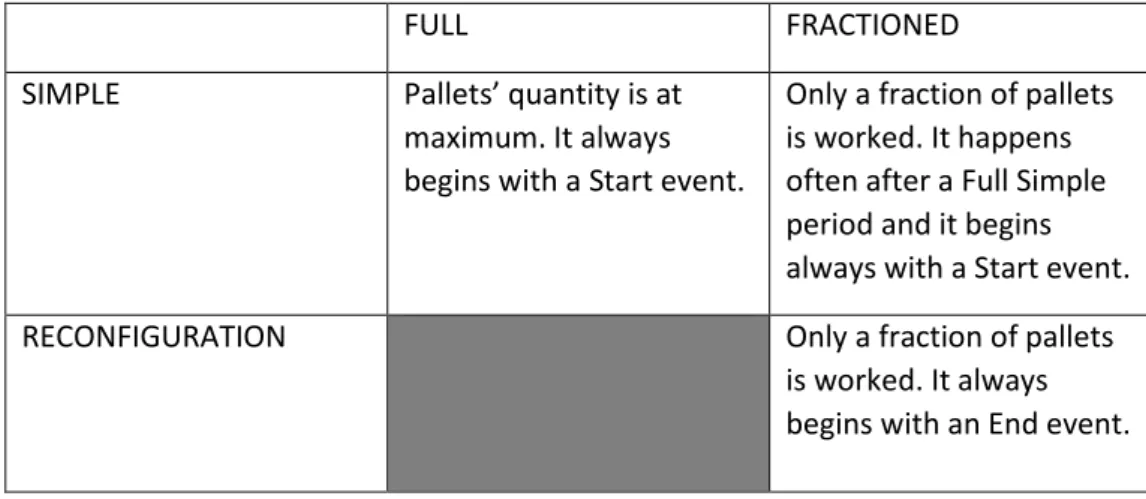
3.5.2 Classification of periods
During each reconfiguration event a certain number of pallet is injected or brought outside the FMS, depending on total number of pallets and ratio of classes in the system. This action provides another classification for periods: full and
fractioned. In a full period, the system operates with the maximum number of
pallets affordable, in a fractioned one only with a fraction of that value.
In Table 3.1 different mixes of period’s types are determined and so all the possible situations in which the system incurs are explained.
The algorithm can approximate adequately the production process of a Flexible Manufacturing System but it is subjected to a simple constraint: Reconfiguration takes part on a whole class each time, so single pallets’ inputs and outputs are not considered.
FULL FRACTIONED
SIMPLE Pallets’ quantity is at maximum. It always begins with a Start event.
Only a fraction of pallets is worked. It happens often after a Full Simple period and it begins always with a Start event.
RECONFIGURATION Only a fraction of pallets
is worked. It always begins with an End event.
4 Transition analysis
4.1 Introduction
The main issue of this analysis and of the algorithm is the transition between periods. This operation must abide by several defined rules. It describes the transition between established periods, called states, which the process must incur. It is connected to the traditional concept of FMS’ production process: production manager defines a list of configurations of the system with their durations and/or demands to fulfill. System is obliged to work following these indications.
This statement can resume transition analysis:
“When a Simple period ends, the transition analysis evaluates which and how many pallets can be introduced in the system: if relationships are compatible with the system state and class suggestion, a Reconfiguration period starts, unless it incurs into a new Simple period or into a blank period.”
4.2 Transition between states
4.2.1 Reconfigurable Transition
This type of method is related to the traditional idea for FMS production that can be resumed as “some pallets for a defined time”. The production is not seen as a continuous and unpredictable change of pallets and periods but it is determined by some fixed periods, called states. The system receives the sequence of states as an input and it analyzes transitions between them. It is crucial to highlight the difference between this method and the previous one: in this case the production process is obliged to pass through predefined states.
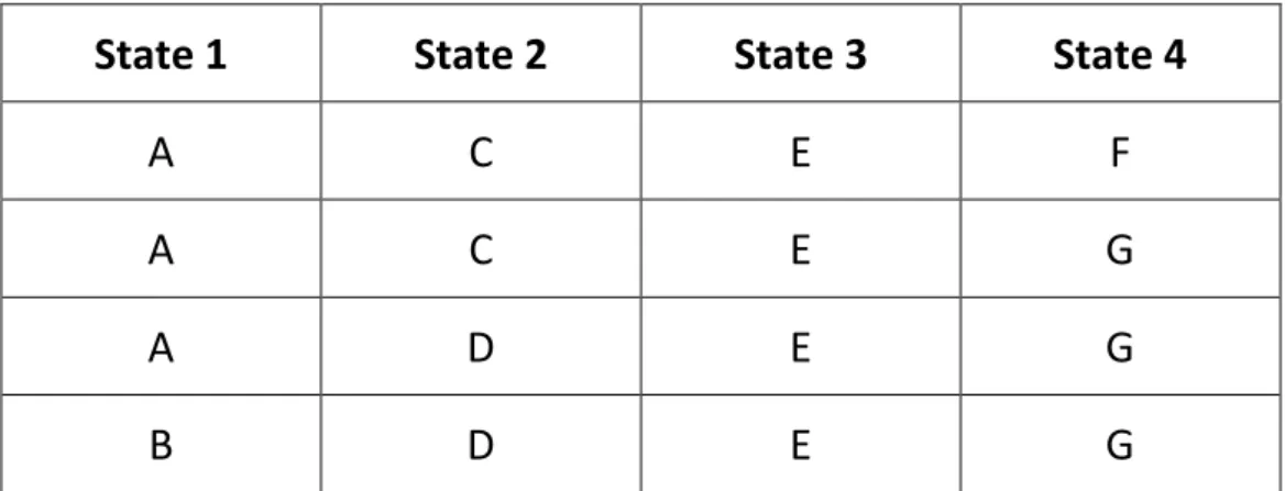
Three elements simply detail a state: type of classes, their ratio, and the total number of pallets. In a simple way, the state designates a set of pallets for each chosen class that should be machined together. The strict rule is that at a certain instant, following the sequence designated, the composition of classes and pallets of the FMS must be the same of the state. A simple example of sequence of states and description of a state can be seen on Table 4.1 and 4.2 respectively.
Once defined these states, that the system receives as an input, the only changeable operation is the passage between a state and the next one.
This method, called Reconfigurable Transition, is adherent to reality and to the actual use of a Flexible Manufacturing System where predefined set of pallets are machined for a certain duration or till the end of demand.
The main criterion used by this method is demand fulfilling: once a class completes its demand, new classes are introduced in the system. The process of introduction of new classes must bring the system to reach a set of pallets and classes equal to the one described by the next state: this procedure can be composed of one or more transitions, depending on states. Since states are fixed, the quantity of possible transitions is fixed and it depends on number of classes and pallets.
The algorithm implemented in MATLAB that manages this transition is
State 1
State 2
State 3
State 4
A
C
E
F
A
C
E
G
A
D
E
G
B
D
E
G
Table 4.1 Sequence of states
Classes
Ratio
Total number of
pallets
A
0.75
4
B
0.25
Transition analysis
31
introduced to reach next state’s composition and it chooses randomly one of them. This list of transitions depends on several factors: the number of free pallets, the number of pallets required in the next state, classes and ratio of actual and next state.
About the number of pallets, it is crucial to consider how many free pallets are available; this number is not always equal to the number of jobs going out of the system. It can be lower if the next state needs less pallets than actual one or it can be higher if the last period is a fractioned one. Classes and ratio of the following state are essential to find a possible transition that brings the system to the next state. The range of transitions between two contiguous states can be easily described by a graph like the one in Figure 4.1.
The set of transitions described in Figure 4.1 is done without regard to the compatibility of classes. Classes are characterized by some relations that determine the chance to machine them together. This research does not face any matter about compatibility, because it is a topic strictly related to specific production processes. For the sake of simplicity, a simple Boolean possibility
matrix is employed, where 1 means that it is possible to machine them together. A simple example is shown in Table 4.3.
A
B
C
D
A
1
0
1
B
1
1
0
C
0
1
1
D
1
0
1
Table 4.3 Boolean Possibility Matrix
The presence of a possibility matrix is a further bond for the algorithm. After the generation of the list of transitions, it analyzes their compatibility using the matrix, to discard inappropriate transitions.
Transition analysis
33
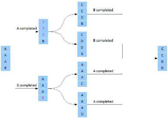
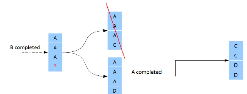
The example of Figure 4.1 can be analyzed using Table 4.3 to get compatible transitions. If the first demand completed is the one of class B, the algorithm must check two couples using the matrix: A-C and A-D. The first one is inappropriate and so the solution A-A-A-C is rejected, while the couple A-D is a possible one and A-A-A-D is a good transition; Figure 4.2 adequately shows the passage.
During this process the algorithm can incur in a remarkable situation: no one of the transitions is compatible. In this case, the number of available pallets is reduced by one unit and the algorithm generates another time a list of transitions and checks their compatibility. This recursive operation could be repeated till the number of pallets becomes equal to zero, in that case the system does not receive any new pallet and it continues production till the end of another class demand. An example of that situation can be taken from example Figure 4.2 when class A is completed. Since there are classes B, C, and D in both the solutions, there is no transition available because A-D is an incompatible couple. The algorithm reduces number of free pallets from three to two and then it creates another time a list of transition. This process is perfectly shown in Figure 4.3.