Alma Mater Studiorum · Universit`
a di Bologna
Scuola di Scienze
Corso di Laurea Magistrale in Fisica del Sistema Terra
Analysis of existing tsunami scenario
databases for optimal design and efficient
real-time event matching
Relatore:
Prof. Stefano Tinti
Correlatore:
Dott. Alberto Armigliato
Presentata da:
Matteo Scarponi
Sessione III
1
Table of contents
1
Introduction
4
2
Case study database
10
2.1 The TRITSU Code 11
2.2 Theory and implementation in brief 11
2.3 Database content 13
2.4 MSDB Content 15
2.5 MSDB storage format 18
2.6 Focus on the Gorringe Bank area 20
3
Analysis of Database
22
3.1 Analysis of frequency content 23
3.2 Analysis of the waveform signals 28
3.2.1 Removing the zeros 30
3.2.2 Shifting procedure 32
3.2.3 Cross-correlation curves 35
3.2.4 Quantifying the relative difference over the fault plane 40
4
The Building algorithm
47
4.1 The reference event 48
4.2 The Building strategy 52
4.2.1 Time gradient 54
4.2.2 Amplitude gradient 54
4.2.3 Exceptions in the building process 57
4.3 The Heart of the work: building the forecast 58 4.3.1 RANDOM1 mode: A completely random selection 60 4.3.2 RANDOM2 mode: A driven selection with some casualties 60
2
4.3.3 ACCURATE SELECTION mode: an ad-hoc built selection 61 4.4 General results for the reference event 63
4.5 Two additional case studies 66
4.5.1 Event located at smaller depth 67
4.5.2 Event located at larger depth 71
5
Focus on the stations with extreme elevations
75
5.1 Top 50 stations 76
5.1.1 Smaller depth event 76
5.1.2 Reference event 86
5.1.3 Larger depth event 93
5.2 Top 2 stations 99
5.2.1 Smaller depth event 100
5.2.2 Larger depth event 103
6
Results and discussion
108
7
References
111
3
Abstract
Pre-computed tsunami scenario databases constitute a traditional basis to the production of tsunami forecasts in real time, achieved through a combination of properly selected Green’s functions-like objects. The considered case-study database contains water elevation fields and waveform signals produced by an arrangement of evenly-spaced elementary seismic sources, covering fault areas relevant in determining the Portuguese tsunami hazard. This work proposes a novel real-time processing for the tsunami forecast production, aiming at the accuracy given by traditional methods but with less time cost. The study has been conducted on the Gorringe Bank fault (GBF), but has a general validity. First, the GBF database is analysed in detail, seeking for remarkable properties of the seismic sources, in terms of frequency content, cross-correlation and relative differences of the fields and waveform signals. Then, a reference forecast for a seismic event placed on the GBF is given, by using all the traditionally available subfaults. Furthermore, a novel processing algorithm is defined to produce approximate forecasts, through a strategic exploitation of the information obtainable by each of the seismic sources, taken in minor number. A further focus on sensible locations is provided. Remarkable results are obtained in terms of physical properties of the seismic sources and time-gain for the forecast production. Seismic sources at depth produce longwave dominated signals, allowing for an optimisation of the database content, in terms of sources required to properly represent seismogenic areas at certain depths. In terms of time cost, an overall improvement is obtained concerning the forecast production, since the proposed strategy gives highly accurate forecasts, using half of the seismic sources used by traditional forecasting methods, which reduces the required accesses to the database.
4
1 Introduction
Over the last 15 years tsunami events have been responsible for a high number of human losses. More than 200,000 people lost their life because of the Indian Ocean tsunami of 26th December 2004 (UNISDR, 2015) and other tsunami events have
severely hit human communities in the following years, e.g. the 29th September
2009 event in the Samoa archipelago, the 27th February 2010 event in Chile, the
25th October 2012 event in the Mentawai islands and the 11th March 2011 event in
Japan. The 26th December 2004 tsunami completely changed the attitude towards
this kind of phenomena and revealed an urgent need for efficient Tsunami Early Warning Systems (TEWS).
Over the years following 2004, many initiatives and coordination groups have been established under the umbrella of the Intergovernmental Oceanographic Commission of UNESCO (IOC-UNESCO) with the aim of improving and developing tsunami warning strategies worldwide. Among these, the ICG/NEAMTWS (see http://neamtic.ioc-unesco.org/) has been established, to develop monitoring and forecasting strategies within the North-Eastern Atlantic, Mediterranean and connected seas area (NEAM).
The NEAM area is characterised by a remarkable distribution of nearshore seismogenic areas, as shown in Figure 1.1, and widespread seismicity, shown in Figure 1.2. Therefore, the time window available for an efficient TEWS to react to hazards is limited to few minutes within this area (e.g. Omira et al., 2009; Tinti et al., 2012a). We stress here that the optimization of time is more than a crucial factor in tsunami early warning practices, which are constituted by hazard detection, impact forecasting, both decision-making and consequent alert dissemination, from local to regional and national level.
5
Figure 1.1: Map of the seismogenic areas of the NEAM region (red areas). The red-coloured polygons represent the seismogenic faults contained in the SHARE-EDSF database (Basili et al., 2013).
Figure 1.2: Seismicity in the southern portion of the NEAM area. The plotted events from the revised ISC Bulletin (http://www.isc.ac.uk,) cover the time period 1960-2016 and are shallower than 50 km.
6
In the early stages of ICG/NEAMTWS, the routinely adoption of the so-called Decision Matrix (DM) has been proposed and it is still used nowadays as a zero-order approximation in the tsunami hazard assessment. The DM is a simple tool, providing the relevant institutions with guidelines to follow in the occurrence of a tsunami hazard. It has the advantage of conveying almost instantaneous instructions, by only requiring the first physical parameters of the new seismic event and it can be used by non-experts in the tsunami-field, as a timely support for decision-making in the hazard occurrence. An example of DM for the NEAM area is given in Appendix A.
Nevertheless, the shortcomings of this approach have been pointed out in various occasions (Tinti et al., 2012b; Tinti et al., 2012c), as the DM approach does not take into consideration the focal mechanism of the earthquake, which strongly determines the tsunamigenic potential of the earthquake itself.
Novel techniques beyond the DM have been investigated over the last years, bringing remarkable improvements towards the production of tsunami forecasts. A possible strategy relies on real-time simulations. This option foresees on-the-fly numerical tsunami simulations as soon as information is provided by the sensor network in the target area. The time needed by the simulations to run depend on a number of factors, roughly belonging to two distinct groups: the first is related to the available hardware and to the software implementation of the desired solving equations, the second has to do with the desired level of detail of the simulations. As for the first group, the continuous and fast improvement of processing units, including the graphical ones (GPUs) and of specific programming languages (e.g. Castro et al., 2015; Macias et al., 2016), the possibility to access small to large computer clusters (e.g. Blaise et al., 2013), are all factors that will allow a continuous reduction of the computation times. On the other hand, the level of detail required for the simulation results represent a key choice: for example, detailed inundation mapping over large coastal areas might request computation times incompatible with the tsunami early-warning needs even when super-computers are available.
7
An alternative approach foresees the building of databases of pre-computed tsunami scenarios. In the emergency phase, suitable forecast algorithms oversee properly selecting and combining the relevant members of the databases in order to forecast the tsunami time evolution in terms of a set of pre-defined metrics. The largest part of the computation time is then shifted to the pre-emergency phase. Several examples of pre-computed databases exist worldwide, built upon different strategies. For instance, the NOAA Center for Tsunami Research has developed the so-called Forecast Propagation Database ( http://nctr.pmel.noaa.gov/propagation-database.html), in which the known earthquake sources over the entire Pacific Basin, the Caribbean and the Indian Ocean have been discretised into unit sources, each consisting in 100-km long and 50-km wide faults with uniform 1 m slip over the fault plane (e.g. Gica et al., 2008). The focal mechanism is determined by the dominating tectonic regime of the area where the sources are found. A similar approach has been adopted by the Center for Australian Weather and Climate Research (Greenslade et al., 2009). A fault-based strategy was also adopted in the framework of the French tsunami warning centre (Gailler et al., 2013): the unit sources are 25-km long and 20-25-km wide, have 1-m uniform slip and their geometries and focal mechanism are tailored on the Mediterranean tectonic sources they discretise. A rather different approach is adopted by other authors (e.g. Molinari et al., 2016 and references therein). The idea is to discretise a given basin into a dense grid of regular cells, each containing an elementary tsunami source which can be Gaussian-shaped, a pyramid, a rectangular prism. In any case, the goal is to make no a-priori assumption about the seismic source geometry, while being able to reproduce any tsunami initial condition by properly combining the elementary cells. Whichever the adopted source selection, the pre-computed databases consist in a number of products regarding different tsunami metrics, typically including water elevation/velocity fields at different times, fields of maximum/minimum water elevation/velocity, water elevation time series at several forecast points. Usually, linear shallow-water wave equations are implemented to compute the tsunami results.
8
The main objective of this thesis is to explore the content of a given database and to seek for its optimization, to minimise the time cost of the associated forecasting procedure, maintaining the accuracy of the forecast itself as high as possible. The case study database has been developed within the European TRIDEC project framework and contains a wide number of pre-computed tsunami scenarios, concerning the North-eastern Atlantic and Western Iberian margin area, obtained by considering multiple elementary seismic sources.
In this case, we decided to focus on the only scenarios related to the well-known seismogenic Gorringe Bank area, located South-West with respect to the Portuguese coasts and presented within Chapter 2.
Together with the description of the focus area, Chapter 2 provides a detailed description of the database content, both in terms of water elevation fields and virtual tsunami waveform signals.
Within Chapter 3, a deep analysis of the properties of the available seismic sources is presented. 2D Fourier analysis is performed over the water elevation fields, while cross-correlation curves and relative differences are computed to the evaluate the similarity between waveform signals produced by different seismic sources. Given the results of these analyses, a consequent strategy is defined within Chapter 4, to understand which aspects of the database can be optimised in terms of accuracy and time cost of the forecast production. Aiming at quantifying how much information can be extracted from a single seismic source, a seismic event of reference and the associated forecast are given.
Then, a building algorithm is strategically defined to produce approximated forecasts, using an increasing finite number of unitary sources, selected via different configurations and criteria. Our main purpose is to evaluate the degree of achievable accuracy in the forecast production, by using the smallest possible number of unitary seismic sources.
This kind of optimisation process has remarkable consequences on the time needed to produce a satisfying accurate forecast in real time.
9
In Chapter 5 a major focus on relevant stations, that produced extreme elevation values within the reference forecast, is discussed to further investigate the performances of the previously defined building strategy.
10
2 Case study database
The case study database, used in this thesis work, is named Matching Scenarios Database (MSDB) and was developed within the European FP7 TRIDEC project (see www.tridec-online.eu).
TRIDEC is a Collaborative project started in 01/09/2010 with a duration of 36 months and ended in 31/08/2013; see Löwe et al. (2013) for a detailed presentation of the project.
TRIDEC had multiple goals, concerning the intelligent management of information during evolving crises, arising both from natural and industrial hazards. It aimed at creating a system-of-services architecture to provide information, decision-making support and careful handling of the warning messages dissemination, with a strong focus also on Information and Communication Technologies (ITC) issues, see Wächter et al. (2012) for ITC aspects within TRIDEC.
Within this project, several efforts have been made towards the tsunami early warning practices and risk mitigation, focusing on certain geographical areas, among which the North-eastern Atlantic and the Western Iberian margin. In this framework, the Tsunami Research Team from University of Bologna developed MSDB as a pre-computed tsunami scenarios database.
The idea underlying this scenario approach (see Sabeur et al. (2013) for a further description) was to use the MSDB to produce real-time tsunami forecasts in terms of waveform signals, by suitably matching a new unkown event with the unitary sources of the database and combining them to produce a real-time forecast. In the following paragraph of this chapter, the fundamental steps in the construction of this database and its content are presented.
11 2.1 The TRITSU Code
As a first step into the description of the Matching Scenarios Database (MSDB), the code used to compute the tsunami scenarios will be briefly presented.
TRITSU code was developed by the Tsunami Research Team of the University of Bologna and ws used to populate the tsunami scenarios database. TRITSU is a slightly modified version of the code called UBO-TSUFD, previously developed by the team and extensively used in several occasions to compute tsunami propagation and inundation, e.g. in the project TRANSFER (http://www.transferproject.eu/), in the project SCHEMA (http://www.schemaproject.org/) and in the study of the 2009 Samoa tsunami as described by Tonini et al., 2011. The main difference between the two codes lie in the fact that TRITSU has been updated to produce standard outputs with agreed format within the TRIDEC project framework.
Beyond this aspect, both codes can compute the solutions of nonlinear shallow-water (NSW) equations over a variable number of nested grids, with different resolutions, depending on the user’s necessities and on the target areas. However, the physical assumptions underlying the implemented model and the numerical techniques used to solve the equations, remain the same in both cases. Hence, the interested reader could be referred to a more comprehensive view of the code development in the work by Tinti and Tonini, 2013.
2.2 Theory and implementation in brief
The code solves both linear and nonlinear shallow-water equations, which approximate the general Navier-Stokes equations. The NSWs are non-dispersive equations as the wave velocity does not depend on the frequency or wavelength but only on the square root of the ocean depth. These equations are obtained under the assumption of fluid incompressibility and pressure hydrostaticity, hence reducing the dimensionality of the problem. In fact, under these assumptions, the vertical component of the velocity becomes negligible and the horizontal
12
components of velocity represent an averaged value over the water column. The NSW equations can be written as:
𝑢𝑡+ 𝑢𝑢𝑥+ 𝑣𝑢𝑦 + 𝑔𝜂𝑥 + 𝑓𝑥 = 0 𝑣𝑡+ 𝑢𝑣𝑥+ 𝑣𝑣𝑦+ 𝑔𝜂𝑦+ 𝑓𝑦 = 0
𝜂𝑡+ (𝑢(ℎ + 𝜂))
𝑥+ (𝑣(ℎ + 𝜂))𝑦 = 0,
with x and y representing the horizontal coordinates, 𝑢 and 𝑣 representing the horizontal components of velocity (averaged along the water column), ℎ the unperturbed height of the water column, 𝜂 the surface displacement from the equilibrium level and 𝑓𝑥 and 𝑓𝑦 the components of the bottom friction.
In these equations, the contribution of the Coriolis term is neglected and therefore their application is valid over spatial domains, whose extension is at most few hundred kilometres and over time domains of few hours of simulation. These conditions adequately suit the NEAM area for the TRIDEC application.
The solution is computed by means of a leapfrog finite-difference numerical scheme over staggered grids, which means that the solutions for velocity components are calculated over a computational grid that is shifted with respect to the computational grid used for sea level elevation. A proper discretization of spatial and time computational domains is essential to guarantee the stability of the leapfrog finite-difference method. The code UBO-TSUFD, which served as a basis for the development of TRITSU, has been tested against different benchmark cases that proved it to be efficient and performant (see Tinti and Tonini, 2013).
TRITSU can furnish the wave propagation solutions both in linear and nonlinear regime over a maximum of eight different nested grids, together with virtual tide gauge records in previously selected grid nodes.
For every run of the TRITSU code, the user should set:
13
The total number of time steps to compute, together with those to be printed as outputs;
The initial condition (also External forcing or landslide sources can be taken into consideration);
other options available, such as deciding whether a smoothing of the initial condition should be performed or not.
For each of the nested grids selected, the associated geographical coordinates must be furnished, together with the spatial and time discretization parameters to define the computational domain and the possible presence of bottom friction.
Eventually, a file indicating the locations at which virtual tide gauge records have to be computed should be included.
2.3 Database content
The parameters of the nested grids used for the MSDB scenarios are given in Table 2.1: Table showing the parameters of the nested grids used for the MSDB database.
Grid Spatial resolution Number of nodes Rows Cols 1 1 km 1342320 1190 1128 2 200 m 4883700 3345 1460 3 200 m 384200 565 680 4 40 m 65550 230 285 5 40 m 54990 234 235 6 40 m 28050 165 170 7 40 m 103750 250 415 8 40 m 60500 275 220
14
The nested grids, shown in Table 2.1: Table showing the parameters of the nested grids used for the MSDB database. have been used to compute the elementary-source water elevation fields for the MSDB database. Grid 1 is the most extended grid with the lowest resolution available. Grid 2 and 3 respectively cover the largest part of the Portuguese coast and Madeira archipelago, with a 200 m resolution. The other 40 m resolution grids have been placed at five target sensible areas: respectively at Cascais, Sesimbra, Sines, Lagos and Funchal, as shown in Figure 2.1.
Figure 2.1: Location of the nested grids presented in Table 2.1.
Furthermore, for each scenario, 1760 virtual tide gauge records have been computed in widespread grid nodes, which we shall call stations from now on. These stations have been distributed along the coastal areas of western Portugal and Gulf of Cadiz, along the north-western coastlines of Morocco and among the coasts of the Madeira archipelago. A few stations have been also deployed in open ocean. The location of the whole set of stations is shown in Figure 2.2.
15
Figure 2.2: The red dots shown in figure, represent the stations at which virtual tide gauge records have been computed for each scenario within the MSDB database.
2.4 MSDB Content
MSDB contains a total amount of 1332 scenarios, each of which has been computed by means of the TRITSU code, within the linear approximation regime of shallow-water equations. Both shallow-water field elevations and tide gauge records have been computed for each one of the scenarios.
Using the linear approximation privileged the aspects regarding open-ocean wave propagation over coastal inundation and run-up, where the nonlinearity would have become a leading factor of the descriptive equations.
16
Within this framework, five seismogenic areas have been defined, based on a previous work by Omira et al. (2009), within which five credible seismic faults have been proposed for the North-eastern Atlantic and Western Iberia region.
The idea, underlying the creation of MSDB, was to use these five seismic faults and their geometry, i.e. strike, dip and rake angles, to define wider planar seismogenic areas, within which tsunamigenic shocks could occur.
Once that the seismogenic areas have been defined, a “tessellation” process has been carried on for each of them. Each area has been divided in a finite number of elementary regular subfaults, with the same geometry of the associated area. The number of subfaults, used to cover a certain seismogenic area, has been fixed by seeking for a compromise between two aspects:
Using numerous subfaults with smaller and smaller dimensions, allows to achieve a higher detail in describing the properties and the behaviour of the target area;
Using a small number of subfaults, hence bigger in dimensions, limits the computational costs required to populate the MSDB database, which becomes smaller in dimensions too. Nevertheless, a too small number of subfaults conveys poor detail in describing the target area.
Based on the magnitude-seismic moment relations by Hanks and Kanamori (1979), designing 20 km long and 10 km wide elementary sources have been regarded as a satisfactory choice. In fact, by assigning an average uniform slip 1.05 over the subfault area and by assuming a rigidity modulus of 30 GPa, each single subfault is comparable to a source of a Mw 6.4 earthquake, which has been considered as a suitable unitary event for the study areas. Given the seismogenic areas of interest and the tessellation parameters, a second tessellation has been defined for every area, by shifting the first one by 10 km along the strike direction. Hence, we have two tessellations for each seismogenic area of interest.
The tessellations are shown in Figure 2.3 and their parameters are given in Table 2.2.
17 MMSFs Number of subfaults Subfaults along the length Subfaults along the width Strike (°) Dip (°) Rake (°) GBF1 & GBF2 108 9 12 53 35 90 HSF1 & HSF2 120 12 10 42.1 35 90 MPF1 & MPF2 108 12 9 20 35 90 PBF1 & PBF2 80 10 8 266.3 24 90 CWF1 & CWF2 250 25 10 349 5 90
Table 2.2: Geometrical parameters for each tessellation in terms of strike, dip and rake angles. The number of subfaults along the length and the width of each tessellation are provided.
Having said that, each subfault has been associated with an initial seafloor vertical displacement, (see Okada,1992), that has been used as initial water elevation field for the TRITSU code.
18
Figure 2.3: MSDB tessellations are shown. For each designed fault, two tessellations have been defined, with one (red one) shifted by 10 km along the strike direction with respect to the other (black one).
2.5 MSDB storage format
To the interested reader, here it is presented how the MSDB content is stored in memory, following the format agreed within the TRIDEC project.
For every tessellation, a folder containing the results of every associated scenario is given. Then, for every single subfault, the results of the computation are stored as follows:
Water elevation fields: We have 8 eight .tar archives containing the solutions computed over the 8 available nested grids. For each grid, the water
19
elevation solution is given every 2 minutes, from the initial condition at time 0 to 240 minutes after the triggering seismic event. Hence we have the results of 4 hours of simulation (the files contain only one sorted column with the elevation values, without the grid coordinates to save storage space). Solutions have been normalised to a 5 m peak-to-peak amplitude to improve the signals to noise ratio.
Virtual tide gauge records: The virtual tide gauge records, at each available station (total number of defined stations is 1760), are given in terms of water elevation values and horizontal velocity components. Here the solutions are given every 15s. Hence, a post-processing interpolation has been performed over the original waveform signal solutions, which are given every 2 minutes.
20 2.6 Focus on the Gorringe Bank area
Despite the large number of studies and of specifically-devised scientific surveys focussing on the SW Iberian margin, the detailed tectonics of the area remains an open and largely debated problem (e.g. Terrinha et al., 2009; Zitellini et al., 2009; Grevemeyer et al., 2017). Similarly, a detailed and widely agreed-upon characterisation of active faults and of their earthquake and tsunamigenic potential is still lacking. The main driving mechanism for the regional tectonics of the area is the NW-SE convergence between the African and Eurasian plates. This convergence does not occur along a single, well-defined tectonic boundary/lineament; rather, the associated deformation appears to be accommodated in a diffuse way along a number of faults placed at different depths and with varying focal mechanism (e.g. Terrinha et al., 2009). On the contrary, seismicity seems to indicate that earthquake occurrence is clustered around a few structures (see Figure 2.4), especially the Gorringe Bank, the Horseshoe Abyssal Plain and the Sao Vicente Canyon (e.g. Custodio et al., 2015; Gravemeyer et al., 2017). Among these, the Gorringe Bank is the most prominent morphotectonic feature observed in the bathymetric maps of the SW Iberian margin. It is an approximately 200-km long, 80-km wide and 5-km high ridge separating the Tagus Abyssal Plain to the NW and the Horseshoe Abyssal Plain to the SE. It strikes approximately normal to the direction of convergence between the African and Eurasian plates.
The Gorringe Bank was taken into account by several authors among the possible structures responsible for the 1755 earthquakes. Some studies, like the one by Grandin et al. (2007) based on the modelling of the distribution of macroseismic intensities reported in SW Iberia, are in favour of the Gorringe Bank as the responsible for the 1755 event, others are instead skeptical on the basis, for instance, of the analysis of tsunami data (e.g. Baptista et al., 2003).
The choice of a fault placed in correspondence with the Gorringe Bank in the present thesis is justified by several reasons. The first is that it is a seismically active structure, as described in Grevemeyer et al. (2017). Secondly, being the most prominent structure in the area, the Gorringe Bank, together with other structures offshore SW Iberia, is being taken into serious account by researchers for both
21
seismic and tsunami hazard assessment for the southern coasts of Portugal, of the Gulf of Cadiz and of Morocco (e.g. Omira et al., 2009; Matias et al., 2013). In particular, Grevemeyer et al. (2017) argue that a fault with approximately the length of the Gorringe Bank has the potential to cause a Mw = 8.7 earthquake, i.e. a 1755 Lisbon-type earthquake and tsunami. Finally, some recent studies (Lo Iacono et al., 2012) mapped and characterised the tsunamigenic potential of a huge mass failure (80 km3 and 35 km of runout), known as the North Gorringe Avalanche
(NGA), along the northern flank of the Gorringe Bank. It is thus evident that the tsunami hazard for the coasts facing the SW Iberian basin is significantly increased in relation of possible large-volume landslides set in motion by moderate-to-large magnitude earthquakes occurring in the Gorringe Bank area (see also Tinti et al., 2012c).
22
3 Analysis of Database
Throughout this chapter, a detailed analysis of the database content properties is presented, focusing on the Gorringe Bank tessellation. The main objective is to study how the waveform signals recorded at stations and the initial water level conditions may vary, by moving the elementary seismic sources over the fault plane.
Each of the initial elevation fields has been subjected to a 2-D Fast Fourier Transform (FFT), while the waveform signals have been compared to each other by means of cross-correlation and relative differences.
The analysis performed has two main purposes:
On one side, we seek for an evaluation of the frequency content of each initial water elevation field. The initial sea level elevation, associated with each tsunami scenario of the database, is determined by the co-seismic seafloor vertical displacement. Comparing the Fourier transforms of different water elevation fields could highlight a dependency of the frequency content on the seismic source parameters, i.e. on the position of the unitary source over the space-oriented fault plane;
On the other side, analysing the waveform signals can let us understand how both the physical propagation process and the position of the seismic source over the fault plane can affect the virtual tide gauge record.
For both aspects, the analysis procedure will be explained and the results relevant to our scope will be highlighted.
23 3.1 Analysis of frequency content
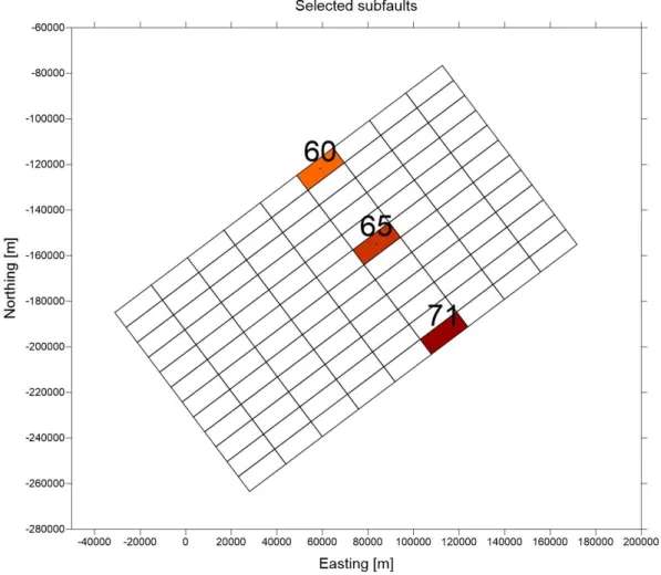
A representative group of three subfaults have been selected, to discuss the results of this preliminary analysis. The subfaults are located over the fault plane at different rows, hence at different depths. The subfaults selected are shown in Figure 3.1.
The depth of the subfaults increases moving down the column, as shown in Table 3.1.
The purpose of this preliminary analysis, is to highlight meaningful differences in the initial sea level conditions, associated with each of the subfaults. It is straightforward that subfaults, located at different depths, induce a different co-seismic vertical displacement of the seafloor. Consequently, we expect that differences in the co-seismic vertical displacement fields, hence in the water elevation fields, can affect the waveforms generated at the various stations.
Figure 3.1: Location of the selected subfaults of the tessellation named GBF1 for this analysis, together with the indexes used to label the subfaults.
24
Subfaults Central Point Depth (m)
60 7868
65 36547
71 70961
Table 3.1: The table presents the depth of the selected subfaults. At the same row, they share the same depth, which increases going down the column.
As expected, initial sea level conditions, shown in Figure 3.2, present remarkable differences in spatial shape and extension. The subfault located in the first row, which is the most superficial one, induce a sea level initial elevation field with smaller spatial extension than the others. The more we move down in the column, and hence the more the seismic source is located at depth, the wider becomes the initial bump at the water surface.
25
Figure 3.2: Initial water elevation fields associated with each of the elementary sources considered. The subfigures present the same spatial arrangement of the subfaults on the fault plane, as shown in Figure 3.1.
26
Each of these initial fields has been subjected to a post-processing procedure to perform a 2-D Fast Fourier Transform (FFT), using the open source python package Numpy for scientific data analysis (see www.numpy.org).
Before computing the FFT, the current fields have been rotated to align their symmetry axis with Easting and Northing directions. Then, a taper has been applied to smoothly bring the elevation field to zero, for elevation values smaller than 1 cm (notice that all the fields from the database present a normalised peak-to-peak amplitude of 5 m).
The 2-D frequency spectrum of each elevation field has been computed and it is shown for each of subfaults considered from Figure 3.3 to Figure 3.5.
By qualitatively analysing the results some remarkable feature can be outlined. As for the elevation fields in Figure 3.2, the frequency spectrum changes with the location of subfaults.
The most remarkable feature is that the frequency spectrum shows a tendency to sharpen and to get close to the origin of the frequency domain, when considering deeper and deeper subfaults (i.e. moving down the column).
The sharpening of the frequency spectrum, around the origin of the frequency domain, means that smaller frequencies, hence longer wavelengths, become increasingly dominant within the frequency content of the initial water elevation field.
This graphical evaluation suggests that the depth of the seismic sources could affect the results of the wave propagation process, in terms of waveform signals recorded at the various stations. In fact, deeper sources produce water elevation fields with higher content of longer wavelengths. Hence, we could expect smaller variations in waveform signals, by moving sources located at larger depth.
This evaluation is meaningful to the purpose of this thesis as, at this step, we shall expect that also the optimal resolution, in terms of fault tessellation, could depend on the location over the fault.
27
Figure 3.3: Frequency spectrum for Subfault 60. Scale is logarithmic to enhance differences. Kx and Ky represent the wavenumber along Easting and Northing direction respectively. This subfault is located at smaller depth with respect to the others.
Figure 3.4: Frequency spectrum for Subfault 65. Scale is logarithmic to enhance differences. Kx and Ky represent the wavenumber along Easting and Northing direction respectively. This subfault is located at medium depth with respect to the fault plane.
28
Figure 3.5: Frequency spectrum for Subfault 71. Scale is logarithmic to enhance differences. Kx and Ky represent the wavenumber along Easting and Northing direction respectively. This subfault is located at the maximum depth availableover the fault plane.
3.2 Analysis of the waveform signals
In this paragraph, the results of the quantitative analyses performed over the waveform signals available are presented. The analyses conducted aim at quantifying the degree of similarity and continuity between signals recorded at the same station, but coming from different seismic sources.
This is rather important to the purpose of this work. In fact, highlighting possible seismic areas over the fault plane, within which the produced waveform signals vary slowly, would help understand how to realise an optimal tessellation of the fault plane.
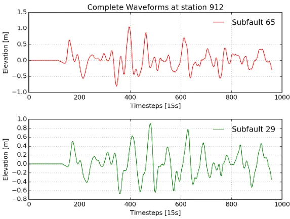
For the sake of clarity, the analysis procedure will be firstly developed over two signals produced at a single station (with index 912), by two different subfaults (with index 29 and 65 respectively).
29
The two subfaults and the station selected, are shown in Figure 3.6.
Figure 3.6: Location of the two subfaults and of the station chosen to illustrate the analysis procedure.
The complete waveform signals produced at the station 912, by the subfaults 29 and 65, as they are stored in the database, are shown in Figure 3.7. The recorded signals range in length from 0 to 961 time steps, each time step having the duration of 15s. Hence, we have four hours of recorded signal.
Before quantitatively comparing the signals to each other, a series of processing operations is required.
30
Figure 3.7: Complete waveform signals produced at the station 912 by the two subfaults considered (29 and 65), for a total duration of 961 time steps (4 hours).
3.2.1 Removing the zeros
A first fundamental operation to perform, is removing the zero-part of the signals, which is present at the beginning of the recording and whose extension depends on the distance of each station from the seismic source associated with the considered scenario.
Concerning the aim of this analysis, we do not want initial zeros to enter the computations over the amplitude of the signals, as we want to perform a meaningful comparison between the oscillations, produced at a single station by different subfaults.
31
Figure 3.8. Complete signals with highlighted initial part constituted by zeros. The blue bar marks the boundary between the oscillations and the part of the signal which has seen no waves yet and hence is cut.
Figure 3.8 shows the zero-part of the signals and the part containing the oscillations, separated by a blue marker. Because of the different location of each subfaults with respect to the same station, the extension of the initial zeros varies from subfault to subfault.
We could refer to the time step, at which the first non-zero signal is detected as the reference time step, which represents a first rough approximation of the tsunami wave arrival time. A precise estimation of the true arrival time would have required a tough frequency analysis, which has not been performed in this work.
Nevertheless, we shall now see the procedure adopted to account for the potential inaccuracy of the reference time step estimation and how to deal with it.
32
3.2.2 Shifting procedure
At the present status, the two signals have been corrected for their initial zeros but they are not yet ready for a meaningful comparison. A further processing is required to account for inaccuracies coming from the cut of the signals at the reference time.
At this part of the analysis, the two signals look like in Figure 3.9 (a).
Figure 3.9: The figure shows: (a) a comparison between the signals that have been corrected only for their initial zeros and (b) a comparison of the two signals after a further processing operation, i.e. a shift to maximise their cross-correlation over the first oscillations.
When comparing two waveform signals recorded at a station, the most meaningful time window is the one containing the first oscillations. This time window, for the considered scenarios within this database, usually extends by no more than one or two hundred time steps from the reference time.
If we look again at Figure 3.9 (a), we can see that the two signals are quite like each other, within the first three or four hundred time steps. Then, the difference starts increasing.
33
In this part of the processing, we should account for the time shift between the two signals, which is clearly visible by looking at the first oscillations in Figure 3.9 (a). Hence, we proceed as follows.
Firstly, we compute the cross-correlation function of the two zero-cleaned signals. Then, we evaluate the necessary shift to align at best the first oscillations of the two signals.
The cross-correlation operation computes an integral, i.e. a summation, over the two signals as a function of their relative shift. For discrete functions f and g, the cross-correlation is defined as follows:
(𝑓 • 𝑔 )[𝑛] = ∑ 𝑓∗[𝑚]𝑔[𝑚 + 𝑛] 𝑚
where f* is the complex conjugate of f, m is the discrete index that ranges through the signals and n the discrete shift between the two signals.
The cross-correlation curve for the two signals previously considered is shown in Figure 3.10. For this computation, the open source python package Scipy for signal analysis has been used (see www.scipy.org/ ).
In this case, cross-correlation is computed only over the first hundred time steps of the zero-cleaned signals, to enhance the weight of the first oscillations.
Once the curve is available as a function of the shift, as shown in Figure 3.10, we seek for the maximum within a suitable window of few steps around the zero shift. The window is used to search for a value of the shift that gives a local maximum, without moving too far from the zero-shift condition.
In fact, our prior-knowledge is that the signals are almost aligned and the correction needed to account for the inaccuracy in reference time step estimation, is likely to be small. Once that we have picked up a suitable maximum, we add in front of one of the signals, depending on the sign of the shift, a shift number of zeros, i.e. we re-define the reference time step.
34
Figure 3.10: Cross-correlation curve for the signal produced at the station 912 by subfault 29 and 65. The curve is computed only over the first hundred time steps of the two signals, to enhance the importance of the fist oscillations recorded. The blue bars represent the window within which we seek for the maximum of the cross-correlation.
Once the cross-correlation over the first hundred time steps of the signal has been maximised through shifting, the two signals look like in Figure 3.9(b). At this point, they are ready to be compared by means of two indicators:
Relative difference: given the two processed signals f and g, we define the relative difference of g with respect to f as:
∆𝑓,𝑔 =
√∑𝑁−1(𝑔𝑖 − 𝑓𝑖)2 𝑖=0
√∑𝑁−1𝑖=0 𝑓𝑖2
Cross-correlation value: it is the cross-correlation computed over the two processed signals with no shift, i.e. we calculate the cross-correlation function over the whole duration of the final processed signals (shown in Figure 3.9(b)) and we take the zero-shift value of the cross-correlation. This is useful to quantify the degree of similarity of the oscillations produced at a single station by two different sources;
35
For the processed signals at the station 912, produced by subfaults 29 and 65, we have the value of relative difference and cross-correlation:
∆29,65= 0.71 𝑥𝐶𝑜𝑟𝑟 = 0.75
3.2.3 Cross-correlation curves
In this paragraph, the xCorr, as previously defined, has been computed over the fault plane.
This time, several couples of subfaults have been strategically selected and the cross-correlation have been computed for each of them.
In this case, all the stations available have been used. Hence, given a single couple of seismic sources, a cross-correlation curve has been generated, showing how the waveform signals produced by the two sources cross-correlate at the various stations.
To show the main results of this analysis, two different subfaults, located at different depth, have been selected as reference subfaults. Their location over the fault plane is shown in Figure 3.11.
36
Once that a reference source has been fixed, we are interested in quantifying how the cross-correlation changes, by computing it with subfaults at increasing distance with respect to the reference.
To this aim, three different configurations have been designed for a single reference subfaults as shown in Figure 3.12.
In these cases, we managed to use both tessellation GBF1 and GBF2, which are shifted by 10 km with respect to each other, providing us with a 10 km per 10 km regular grid, over which every point represents the epicentre of an elementary seismic source.
For each configuration, four subfaults are chosen equidistant from the reference, with the distance being 10 km, 20 km and 30 km for each configuration.
The results are shown for the considered reference subfaults, 75 and 80, as their behaviour well represents the behaviour seen along their rows during this work. By looking at the subfault 75, we see that values of the cross-correlation curves are close to one within the first configuration (Figure 3.13), i.e. when the neighbour subfaults are at 10 km distance. Values become lower when the distance of subfaults increases to 20 km and 30 km (Figure 3.14 and Figure 3.15). The waveforms concerned with the Madeira archipelago (from 1400 on in the previous figures), show a tendency of decreasing faster in terms of cross-correlation. A
Figure 3.12: The figure shows the three configurations adopted for calculating the cross-correlation curves. The central shaded subfault is the reference one. As can be seen, by using GBF1 (red shaded grid and red subfaults) and GBF2 (green shaded grid and green subfaults) tessellations, we have a 10 km per 10 km grid. The subfaults to be cross-correlated with the reference are chosen at increasing distances every 10 km, as can be seen from left side to right side of the figure.
37
common feature throughout the three configurations, is that cross-correlation computed with subfaults located higher (i.e. at smaller depth) than the reference cell, shows the lowest values. While cross-correlation computed with faults located on the left and on the right, i.e. at the same depths the reference subfault, presents the highest value of cross-correlations throughout the three configurations. The features can be seen also by looking at three figures concerning the reference subfault number 80, which is located deeper in the fault plane than subfault 75. A remarkable feature is that, given a fixed configuration and a given choice of the subfault to correlate with the reference, the subfault 80 shows cross-correlation values systematically higher than the ones shown by subfault 75.
This demonstrates that at major depths, the closer the subfaults are, the more similar are the signal they produce, hence revealing that the tessellation of the deeper area of the fault could be subject to an optimization process.
Figure 3.13: Cross- correlation curves for reference subfault number 75, obtained in the first configuration (10 km separation). The legend tells which subfault has been cross-correlated with the reference.
38
Figure 3.14: Cross- correlation curves for reference subfault number 75, obtained in the second configuration (20 km separation). The legend tells which subfault has been cross-correlated with the reference.
Figure 3.15: Cross- correlation curves for reference subfault number 75, obtained in the third configuration (30 km separation). The legend tells which subfault has been cross-correlated with the reference.
39
Figure 3.16: Cross- correlation curves for reference subfault number 80, obtained in the first configuration (10 km separation). The legend tells which subfault has been cross-correlated with the reference.
Figure 3.17: Cross- correlation curves for reference subfault number 80, obtained in the second configuration (20 km separation). The legend tells which subfault has been cross-correlated with the reference.
40
Figure 3.18: Cross- correlation curves for reference subfault number 80, obtained in the third configuration (30 km separation). The legend tells which subfault has been cross-correlated with the reference.
3.2.4 Quantifying the relative difference over the fault plane
Similarly to the previous sections, relative differences in waveform signals, produced by different seismic sources over the fault, have been computed. To this aim, a reference row and a reference column over the fault have been chosen as shown in Figure 3.19.
41
Figure 3.19: The figure shows the reference column (green column on the left) and the reference row (blue row on the right), chosen as references in computing relative differences between subfaults. Once a row has been chosen, we calculate differences between the green reference of subfaults for that row, at increasing distances. Similarly, once that a column has been chosen, we calculate differences selecting subfaults at increasing distances from the blue reference for that column.
Then, we proceed as follows in selecting the subfaults to be compared:
In this case, we proceed by taking a single row at a time and, successively, a single column at a time.
For every fixed row, we have a reference subfault, i.e. the central one, and we start computing relative differences in waveform signals, by considering subfaults of increasing distance from the reference.
By using both tessellation GBF1 and GBF2, we manage to achieve 8 different selections of subfaults at gradually increasing distance from the reference.
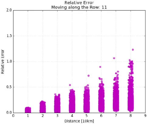
The relative errors along a fixed column are computed selecting subfaults in a similar manner, by increasing the distance from the central row of reference. The results are shown from Figure 3.20 to Figure 3.25. They are given as scatter plots representing the relative difference between a subfault, at a given distance with respect to the reference, for every single station available.
42
Figure 3.20 Relative difference at various distances from the central element of the first row, moving along the same row. Each dot represents the relative difference associated with a single station.
Figure 3.21: Relative difference at various distances from the central cell of the fifth row, moving along the same row. Each dot represents the relative difference of a single station.
43
Figure 3.22: Relative difference at various distances with respect to the central element of the last row.
Figure 3.23: Relative difference with respect to central element of the first column at various distances, moving along the column. Each orange dot represents a single station.
44
Figure 3.24: Relative difference with respect to central element of the fourth column at various distances, moving along the column. Each orange dot represents a single station
Figure 3.25: Relative difference with respect to central element of the eighth column at various distances, moving along the column. Each orange dot represents a single station.
45
Some remarkable results can be highlighted by looking at the relative differences computed both along the columns and the rows:
As expected, the relative difference in produced signals, with respect to central reference, increases at increasing distances, both along the columns and the rows. In fact, at a certain distance, the relative difference reaches high values around 1 or more than 1, as can be seen by inspecting graphs from Figure 3.20 to Figure 3.25. Even if all configurations, both along columns and along rows, present increasing relative differences at increasing distances, the rate at which the difference increases may change, depending on the configuration considered. In fact:
Moving along different columns does not provide any remarkable difference in the difference growth, as can be seen in Figure 3.23, Figure 3.24 and Figure 3.25.
Moving along different rows provides very different growing trends for the relative differences. In the most superficial row, the average difference is very high, and some stations present differences over 1 also at a 10 km distance, as can be seen in Figure 3.20.
By considering a deeper row, shown in Figure 3.21, we can see that the growth of difference in waveform signals, obtained while moving along the row itself, is a minor growth and differences are generally lower than the ones obtained at the first superficial row.
By considering the deepest row available, shown in Figure 3.22, we can see that relative differences have sharply decreased with respect to the previous cases and their growth is smaller when moving along the same row.
46
The results of these analyses, conducted both over the water elevation fields and over the waveform signals generated by the elementary sources, suggest that an optimization of the unitary sources’ arrangement can be achieved, especially working along the rows.
In fact, subfaults along the same rows share remarkable properties. On one side, along the same row we have the same average frequency content and we have seen that, moving along a single fixed row, cross-correlation values are higher and differences are smaller.
Moreover, these analyses show that the signals produced by deeper rows present larger values of cross-correlation and lower differences, even with respect to the rows located at smaller depths.
These evident features have directly affected and driven the development of our optimization strategy as we have chosen to work mainly along the rows to search for suitable optimizations.
Given these preliminary results, in the following chapters our work and its main results are presented.
47
4 The Building algorithm
Producing a forecast in terms of waveform signals at sensible locations, e.g. along the coast, is a novel approach with respect to the routinely adopted Decision Matrix.
In the first part of this chapter, a reference tsunamigenic event is proposed and its expected waveform signals are produced, by matching the event with the elementary seismic sources of the MSDB database.
Based on the results of the previous analyses, a “Building” algorithm is designed and suggested to optimise the forecast production.
The main objective is to approximate at best the reference forecast, by using a smaller number of subfaults upon a strategic processing.
The goal of the Building process is to search for a better exploitation of the information, obtainable from a smaller number of elementary sources. Different configurations of subfaults will be considered to eventually define a strategy towards the optimization of the forecasting procedure.
The first paragraph of the chapter is devoted to the description of the reference event and the associated reference forecast.
In the second the strategy of the building process is explained by means of a simple case with two subfaults and a single station.
In the third paragraph the strategy is applied and generalized all over the surface of interest and the results are discussed.
48 4.1 The reference event
The reference event is a Mw 8.1 earthquake located over the GBF plane. It is modelled as a homogeneous slip distribution over a rectangular area. The source parameters are given by Hanks and Kanamori (1979) and shown in Table 4.1, together with easting and northing coordinates.
Reference Event Mw 8.1 Slip (m) 5.4 Length (m) 189670.6 Width (m) 51404.4 Easting (m) 72755.16 Northing (m) -173304.1 Depth (m) 42282.5
Table 4.1 Source parameters of the reference seismic event
The considered event is consistent with the tsunamigenic potential of the area and its historical events (Johnston, 1996). The horizontal projection of the seismic source is shown in Figure 4.1 The figure shows the reference event located over the GBF plane, matching the underlying unitary sources. In this figure, the projection at the horizontal surface is shown both for the considered seismic event and the GBF tessellation. The epicentre location is shown, together with some sample stations along the coastal line. together with some sample stations located along the coast.
49
The reference event is matched with the underlying 45 regularly-spaced subfaults, that have been highlighted in red in Figure 4.1.
Figure 4.1 The figure shows the reference event located over the GBF plane, matching the underlying unitary sources. In this figure, the projection at the horizontal surface is shown both for the considered seismic event and the GBF tessellation. The epicentre location is shown, together with some sample stations along the coastal line. The epicentre is far no more than few hundred kilometres from the Portuguese coast and the North-western Morocco coast. The subfault in red have been selected to produce the reference forecast.
50
Being the tsunami equations linear, the expected signals induced by the waves propagation are obtained by summing over the matched unitary sources’ signals, whose amplitude has been corrected to guarantee the conservation of seismic moment (before correction, the elementary signals are associated with 1 m slip over the elementary sources).
In this way, a reference forecast is produced by summing over the elementary sources involved in the event.
An example of forecasted waveform signals at four stations is shown in Figure 4.2
Example of waveform signals forecasted for the new event using all the 45 subfaults available, at four different stations.
51
Figure 4.2 Example of waveform signals forecasted for the new event using all the 45 subfaults available, at four different stations. shows the forecasted signals concerning four sample stations, two of which, the 651 and 901, are located at the Portuguese coast, while the other two, the 1251 and the 1351, are located at the Morocco coast.
By looking at these reference forecasts, tsunami waves are expected to impact Portuguese coasts within 20-minute time and Morocco coasts within 50-minute time.
Producing these forecasts has a time cost. Accessing the database for the 45 matched elementary sources and reading the associated 1760 signals (one for each station available), has required 62.17 seconds, hence little more than a minute. The specification of the used CPU is:
Intel ®Core™i7-4790 CPU @ 3.60GHz
The order of the minute becomes relevant when compared to an expected impact within 20 minutes.
This thesis work suggests that this time cost can be reduced, by paying an affordable price in terms of accuracy with respect to the reference forecast. To explore this possibility, a building algorithm is presented in the next paragraphs. The purpose of the algorithm is to use a smaller number of subfaults (less than 45) to approximate the refence forecast. Different configurations of subfaults are tested and the performance of the building process evaluated.
52 4.2 The Building strategy
We refer to a building process when, given an unknown subfault, we try to reconstruct the signal it produces at a certain station, using the signals produced by neighbour subfaults.
We start considering a simple case with two known subfaults, i.e. 28 and 52, and a single station, 901. They are shown in Figure 4.3.
Figure 4.3 Simple configuration to explain the Building strategy. We consider a single station (901) and two known subfaults (ruby red ones), which we want to use to build the waveform signal associated with the unknown target subfault 40 (sea green).
By using the signals produced by subfaults 28 and 52 at the given station, we want to build an approximation of the signal, that would have been produced by the unknown subfault 40.
The known signals produced by 28 and 52 are shown in Figure 4.4, where the blue bar represents the reference time step as defined in paragraph 3.2.2. In this case, we have:
𝑡28= 150 time steps 𝑡52= 140 time steps
53
To build the signal of the subfault 40, we must account for two fundamental aspects:
The reference time: The oscillations produced at the given station, by the three different subfaults, begin after a suitable amount of time, necessary for the tsunami wave to travel from the source to the considered station. Hence, we must define a proper reference time for the unknown subfault when building its signal;
The oscillations: The oscillations produced at the given station vary with a certain continuity throughout the elementary sources (as analysed in chapter 3) and we have to define a proper interpolation/extrapolation operation to build the oscillations of the unknown subfault;
Figure 4.4: The figure shows the known waveform signals of subfaults 28 and 52, together with the blue bar that marks the first non-zero value of the signal.
54
We take care of these two aspects in a separate way by defining two gradients and the target signal is built by merging the results of two linear expansions.
4.2.1 Time gradient
Given two known subfaults, the 28 and the 52 in this case, we define time gradient as the difference of reference time steps over the distance of the two subfaults:
𝑔𝑟𝑎𝑑𝑡 = 𝑡52− 𝑡28 𝑥52− 𝑥28
Where 𝑥52 , 𝑥28 represents the position of the subfaults along the row.
The gradient is defined with an orientation as we take the first subfault along the row and we subtract it to the second.
In this way, we can compute the approximate time reference by means of a linear expansion starting from the first subfault:
𝑡40= 𝑡28+ 𝑔𝑟𝑎𝑑𝑡 ∗ ( 𝑥40− 𝑥28 ) = 145 𝑡𝑖𝑚𝑒 𝑠𝑡𝑒𝑝𝑠
where 𝑥40 is the position of the target subfault along the row. We obtained a first estimate for 𝑡40 , which may need a little further correction, depending on the shift between the oscillations of signals 28 and 52.
4.2.2 Amplitude gradient
We then define a second gradient in terms of the amplitude of the oscillations. To this purpose, we consider only the oscillatory part of the signals, delimited by the blue bar in Figure 4.4.
Let 𝑓52 and 𝑓28 be the non-zero signals associated with subfaults 52 and 28
respectively. We then define the amplitude gradient as:
𝑔𝑟𝑎𝑑𝑓 = 𝑓52− 𝑓28 𝑥52− 𝑥28
This is a point-to-point difference and, before computing it, the two signals are normalised in length and subjected to the same shifting procedure described in paragraph 3.2.2, to account for possible shifts between first oscillations. If a shift is required, hence a time reference of the two signals is re-defined, and 𝑡40 is properly
55 Therefore, we can write:
𝑓40= 𝑓28+ 𝑔𝑟𝑎𝑑𝑓 ∗ (𝑥40− 𝑥28)
An example of gradf for this sample case is given in Figure 4.5. Point-to-point
difference between the non-zero signals produced by subfaults 28 and 52. As it can be noticed, the gradient is small within the few first hundred time steps, then it reaches instability as the signals become different.
At this point the target signal for subfault 40 is obtained by merging the oscillatory part 𝑓40, with a suitable number of zeros given by 𝑡40.
56
Figure 4.6 Comparison between the true signal produced by the subfault 40 at the station 901, with its approximation shows the comparison between the true forecasted signal for subfault 40 at station 901 and its approximation, built by using the known neighbour subfaults.
The approximate signal shows some inaccuracies, but it performs well in recovering the true reference time step, the frequency and the amplitude of the oscillations within the first few hundreds time steps.
This is a remarkable result in terms of optimization of the forecasting procedure as we managed to obtain three useful signals by accessing the database only twice, for subfault 28 and 52.
Figure 4.6 Comparison between the true signal produced by the subfault 40 at the station 901, with its approximation.
57
In the next paragraphs, we will generalise this approach over the 45 matched subfaults, used to produce the reference forecast, and we will try to approximate it by using a smaller number of subfaults from the database.
4.2.3 Exceptions in the building process
Every time an amplitude gradient is computed between two known subfaults, the cross-correlation is computed over the first oscillations to account for a potential shift, for every station available.
If the normalised cross-correlation maximum is below the threshold value of 0.5, neither amplitude or time gradients are defined between the two subfaults for the considered station. In this case, the target signal is estimated as the simple mean of the two known signals.
Adopting a simple mean in building an unknown signal coincides with performing no building at all and just increasing the amplitude of the known signals. When building a forecast, this means only accounting for the conservation of the seismic moment without any further operation.
58
4.3 The Heart of the work: building the forecast
In this chapter the generalization of the building process over the fault plane is presented.
To understand the functioning of the algorithm, let us suppose we have a certain amount of missing subfaults, underlying a tsunamigenic event as shown in Figure 4.7: The reference seismic event is shown over the tessellation. Some subfaults, underlying the seismic event area, are supposed to be missing for this example. The building process is applied over the fault area to fill the relevant vacancies:
Figure 4.7: The reference seismic event is shown over the tessellation. Some subfaults, underlying the seismic event area, are supposed to be missing for this example. The building process is applied over the fault area to fill the relevant vacancies.
The reference forecast is produced by summing over all the complete set of 45 subfaults from the database. Our objective is then to estimate the waveform signals, associated with the missing subfaults, and to produce an approximate version of the original forecast.

![Figure 2.4: Seismicity map for the SW Iberia [ISC bulletin].](https://thumb-eu.123doks.com/thumbv2/123dokorg/7427008.99337/22.892.151.743.538.1025/figure-seismicity-map-sw-iberia-isc-bulletin.webp)