Bayesian Hierarchical Gaussian Process Model: an Application to Multi-Resolution Metrology Data

(1)

POLITECNICO DI MILANO

Scuola di Ingegneria dei Sistemi

Corso di Laurea Specialistica in

Ingegneria Matematica

Bayesian Hierarchical Gaussian Process Model:

an Application to Multi-Resolution Metrology Data

Relatore: Ch.ma Prof. Bianca Maria COLOSIMO

Tesi di Laurea Specialistica di:

Lucia DOLCI Matr. 675215

(2)

Ringraziamenti

Ringrazio la mia relatrice Prof.ssa Bianca Maria Colosimo, della Sezione Tecnolo-gie e Produzione del Dipartimento di Meccanica, per la ﬁducia che ha riposto in me nell’assegnarmi questo stimolante progetto di ricerca, nonostante il mio “tormen-tato percorso accademico”. Le sono grata inoltre per le appassionate discussioni in occasione dei nostri incontri e per avermi introdotta, con il suo corso di Ge-stione Industriale della Qualit`a, al mondo della statistica applicata ai problemi industriali.

Ringrazio l’Ing. Paolo Cicorella, studente della Scuola di Dottorato, insostituibile aiuto in questi questi mesi di lavoro presso la sezione Tecnologie e Produzione del Dipartimento di Meccanica. La sua disponibilit`a, la sua grinta e i suoi consigli sono stati indispensabili.

Un grazie sincero all’Ing. Luca Pagani, per la sua pazienza e il suo inesauribile interesse per qualunque problema sottopostogli.

Un aﬀettuoso pensiero va anche a tutti gli studenti e ricercatori, conosciuti presso il laboratorio della Sezione, per la compagnia di questi mesi.

Dedico questo traguardo a mia mamma, a mio fratello e a mia zia, ai quali spetta il ringraziamento più grande: per essermi stati accanto in ogni momento, per le infinite possibilità che mi hanno riservato e per aver creduto in me.

Ringrazio inﬁne i miei amici storici dell’arte, per avermi sopportata in questi ul-timi “mesi bayesiani”, nonostante non abbia fatto altro che parlare di cose a loro incompresibili.

(3)

List of Figures

1.1 The eﬀect of varying the power parameter on the sample paths of a GP with power exponential correlation function. Four draws from a GP(µ, σ2, θ, p), with µ = 0, σ2 = 1.0, θ = 1.0 and respectively

p = 2.0 (a), p = 0.75 (b) and p = 0.2 (c) [SWN03]. . . . 23 1.2 The eﬀect of varying the scale parameter on the sample paths of a

GP with power exponential correlation function. Four draws from a GP(µ, σ2, θ, p), with µ = 0, σ2 = 1.0, p = 2.0 and respectively

θ = 0.5 (a), θ = 0.25 (b) and θ = 0.1 (c) [SWN03]. . . . 24

3.1 Histograms of β_l and σ2

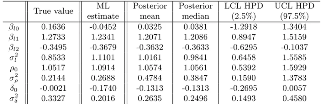
l. The purple lines represent the posterior medians, the cyan lines the true values of the parameters, the red lines their ML estimates, the black lines the 95% credibility HPD limits (Simulated data - I). . . 70 3.2 Histograms of ρ0, δ0, σρ2 and σδ2. The purple lines represent the

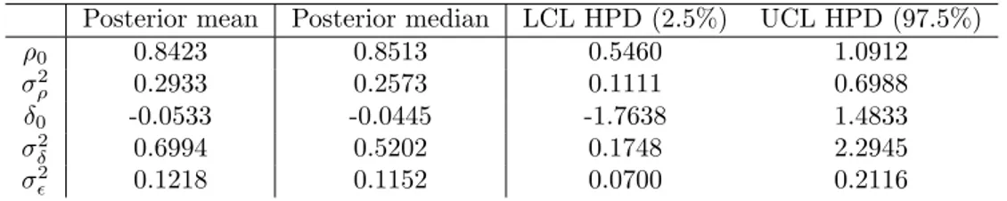
posterior medians, the cyan lines the true values of the parameters, the red lines their ML estimates, the black lines the 95% credibility HPD limits (Simulated data - I). . . 71 3.3 Histograms of ρ0, δ0, σρ2 and σδ2. The purple lines represent the

posterior medians, the black lines the 95% credibility HPD limits (Example 1 from [QW08]). . . 74 3.4 Graphical representation of the central portion of the Matlab

func-tion peaks. . . 78 3.5 Representation of the simulated LE and HE data with respect to

the wireframe surface of the analytic function. . . 78 3.6 Histograms of ρ0, δ0, σ2ρ and σδ2. The purple lines represents the

posterior medians, the black lines the 90% credibility HPD limits (Simulated data - II). . . 81

(8)

LIST OF FIGURES 7

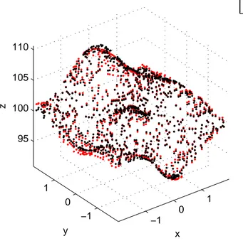
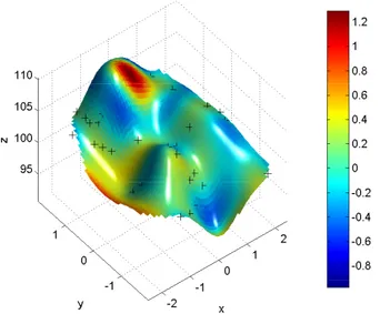
3.7 Representation of the clouds of the predicted points (red) computed using the BHGP model and the corresponding points of the true function (black) (Simulated data - II). . . 82 3.8 Interpolated error plot: it displays the magnitude of the

predic-tion error ytest− ˆyBHGPh on the shape of the interpolated predicted surface. Cold colors indicate negative prediction errors, i.e. the predicted points are overestimates of the testing measured points. Warm colors indicate positive prediction errors, i.e. the predicted points are “impossible” as they lie under the measured surface (model validation with simulated data - II). . . 83

4.1 Methods of geometric data acquisition [Wec+09]. . . 90 4.2 MScMS-II architecture. The dashed lines represent visual links

be-tween sensor nodes and retro-reﬂective markers (indicated as A and B) of the handheld probe. The Bluetooth connection is established between each node and the processing system [GMP10a]. . . 94 4.3 IR sensor: an IR camera is coupled with an IR LED array to locate

passive retro-reﬂective targets [GMP10a]. . . 96 4.4 Virtual reconstruction of the working layout. The black lines

rep-resent the camera “ ﬁeld of sensing” and the pink lines identify the working volume that, according to the triangulation principles, is the volume of intersection of the ﬁeld of sensing of at least two cameras.[GMP10a]. . . 97 4.5 Mobile measuring probe. [GMP10a]. . . 97 4.6 Scheme of the data processing system. The calibration procedure is

responsible for determining positions and orientations of the IR sen-sors within the working environment. The localization procedure, implementing a triangulation method, reconstructs the 3D coordi-nates of the touched point by locating the passive markers on the measuring probe. A further step of data elaboration is implemented to coordinate the data processing operations (acquisition and elabo-ration), according to the purpose of the measurements (single-point, distance or geometry reconstruction). In this process, n is the num-ber of measured points and np is the number of points needed to perform the processing. [GMP10a]. . . 99

(9)

LIST OF FIGURES 8

4.7 Graphical representation of the localization problem when a setup of four cameras (nc = 4) is used to reconstruct the 3D position of two markers (m = 2). xci (with i = 1, , 4) and xM j (with j = 1, 2) refer to the 3D coordinates of the i-th camera center and the j-th marker, respectively. Point uij represents the 2D projection of

xM j onto the image plane of the i-th camera. It corresponds to the intersection of the camera view plane πi with the projection line of

xM j (i.e., the line passing through the 3D point and the camera center) [GMP10a]. . . 100 4.8 Coordinate-Measuring Machine CMM DEA Iota 0101 used at the

metrology laboratory of DISPEA, Torino. [Fra+10]. . . 102

5.1 The measured object [Fra+10]. . . 106 5.2 The detail of the measured surface of the hood and the front bumper

[Fra+10]. . . 107 5.3 Representation of the point clouds of the measurements acquired

with the MScMS-II system (red) and the CMM (blue). Their re-spective markers are represented as black Xs and stars. . . 108 5.4 Representation of the point clouds of the measurements acquired

with the MScMS-II system (red) and the CMM (blue) after the registration procedure with the Matlab function procrustes. . . . 109 5.5 Representation of the point clouds acquired with the MScMS-II

(red) and the CMM (blue) in the three data conﬁgurations. . . 112 5.6 Representation of the clouds of the predicted points (red) and the

corresponding testing set of CMM points (blue) for all the three analyzed data conﬁgurations. . . 116 5.7 Interpolated error plot: it displays the magnitude of the

predic-tion error ytest− ˆyBHGP_h on the shape of the interpolated predicted

surface. Cold colors indicate negative prediction errors, i.e. the predicted points are overestimates of the testing measured points. Warm colors indicate positive prediction errors, i.e. the predicted points are “impossible” as they lie under the measured surface (Data conﬁguration 1). . . 117

(10)

LIST OF FIGURES 9

5.8 Interpolated error plot: it displays the magnitude of the predic-tion error ytest− ˆyBHGPh on the shape of the interpolated predicted surface. Cold colors indicate negative prediction errors, i.e. the predicted points are overestimates of the testing measured points. Warm colors indicate positive prediction errors, i.e. the predicted points are “impossible” as they lie under the measured surface (Data conﬁguration 2). . . 118 5.9 Interpolated error plot: it displays the magnitude of the

predic-tion error ytest− ˆyBHGP_h on the shape of the interpolated predicted

surface. Cold colors indicate negative prediction errors, i.e. the predicted points are overestimates of the testing measured points. Warm colors indicate positive prediction errors, i.e. the predicted points are “impossible” as they lie under the measured surface (Data conﬁguration 3). . . 119 5.10 Box-plots of the Square Root Squared prediction Errors computed

(11)

List of Tables

3.1 Sampled values for the parameters (Simulated data - I). . . 62 3.2 True values, posterior means and medians of the parameters β_l, σ2_l,

ρ0, δ0, σρ2 and σδ2 and their respective 95% credibility HPD limits (Simulated data - I). . . 69 3.3 Posterior mean and median of the parameters ρ0, δ0, σρ2 and σδ2

and their respective 95% credibility HPD limits (Example 1 from [QW08]). . . 73 3.4 Prediction results at the ntest = 12 testing points. yh test is the

true HE response; ˆyBHGP

h test is the response predicted using the BHGP model LPL and UPL are the 95% prediction limits (Example 1 from [QW08]). . . 76 3.5 Prediction results at the ntest = 12 testing points computed using

the BHGP model are compared to the other two predictions ˆySWN_test and ˆyRasmussen

test . Such responses are computed using only the LE data

with the predictive density proposed by [SWN03] and the method proposed by [RW06] respectively (Example 1 from [QW08]). . . 76 3.6 Posterior means and medians of the parameters ρ0, δ0, σ2ρ and

σ2_δ and their respective 90% credibility HPD limits obtained with BHGP model (Simulated data - II). . . 80 3.7 Ranking of the compared prediction methods sorted by decreasing

predictive performance according to the results of the Sign Tests performed on the diﬀerences of the SMPs (Simulated data - II). . . 86

4.1 Deﬁnition and description of LMS basic requirements [Fra+09], [GMP10a]. . . 91 4.2 Innovative technical and operational characteristics of the

MScMS-II [GMP10b]. . . 93

(12)

LIST OF TABLES 11

4.3 Qualitative comparison of optical-based distributed systems for large-scale metrology and quantitative estimate of their economic impact [GMP10a]. . . 95 4.4 Technical characteristics of the sensors in the MScMS-II [GMP10b]. 96 4.5 Technical characteristics of the CMM DEA Iota 0101 used at the

metrology laboratory of DISPEA, Torino. . . 103

5.1 Comparison of the prediction results in terms of Square Root Mean Squared Prediction Error. . . 120 5.2 Ranking of the compared prediction methods sorted by decreasing

predictive performance according to the results of the Sign Tests performed on the diﬀerences of the SMPs (Data conﬁguration - II). 122 5.3 Ranking of the compared prediction methods sorted by decreasing

predictive performance according to the results of the Sign Tests performed on the diﬀerences of the SMPs (Data conﬁguration - II). 123

(13)

Abstract

In the present work we discuss and extend an existing Bayesian Hierarchical Gaus-sian Process Model (BHGP) used to integrate data with different accuracies. The low-accuracy data are the deterministic output of a computer experiment and the high-accuracy data come from a more precise computer simulation or a physical experiment. A Gaussian process model is used to fit the low-accuracy data. Then the high-accuracy data are linked to the low-accuracy data using a flexible ad-justment model where two further Gaussian processes perform scale and location adjustments. An empirical Bayesian approach is chosen and a Monte Carlo Markov Chain (MCMC) algorithm is used to approximate the predictive distribution at new input sites. The existing BHGP model is then extended in order to model the more general situation where also the low accuracy data come from a physical experiment. A measurement error term needs to be included in the model for the low-accuracy data and the MCMC prediction method is accordingly adjusted. The BHGP model is implemented in Matlab and a validation study is performed to verify the developed code and to evaluate the predictive performance of the model. The extended BHGP model is then applied to a set multi-sensor metrology data in order to model the surface of an object. The low-accuracy data are measured with an innovative optical-based Mobile Spatial Coordinate Measuring System II (MScMS-II), developed at Politecnico di Torino, Italy, and the high-resolution data are acquired with a Coordinate-Measuring Machine (CMM). Comparing the BHGP model with other existing methods allows us to conclude that significative improvements (by 11%− 22%) in terms of prediction error are achieved when low-resolution and high-low-resolution data are combined using an appropriate adjustment model.

(14)

Sommario

Nel presente lavoro si analizza e si estende un modello bayesiano gerarchico che sfrutta i processi gaussiani (BHGP) con lo scopo di integrare dati con diversa accu-ratezza. I dati a bassa accuratezza provengono da un esperimento computazionale deterministico, mentre quelli ad elevata accuratezza da una simulazione numer-ica più precisa o da un esperimento fisico. Un processo gaussiano modella i dati a bassa accuratezza, mentre un modello flessibile di aggiustamento collega i dati molto accurati a quelli poco accurati, sfruttando due ulteriori processi gaussiani che svolgono la funzione di parametri di scala e di localizzazione. Si adotta un approccio bayesiano empirico per fare inferenza sui parametri del modello e si sfrutta un algoritmo Markov Chain Monte Carlo (MCMC) per approssimare la distribuzione a posteriori predittiva in corrispondenza di nuovi punti sperimentali. Il modello BHGP esistente viene esteso in modo da poter essere applicato al caso più generale in cui anche i dati a bassa accuratezza provengono da un esperimento fisico. Un temine di errore casuale è introdotto nel modello dei dati a bassa ac-curatezza e i passi dell’algoritmo MCMC devono essere corretti di conseguenza. Dopo aver implementato il modello in Matlab, si svolge uno studio di validazione per verificare la correttezza del codice e le prestazioni del modello in termini pred-ittivi. Il modello BHGP viene infine applicato a dati di metrologia, provenienti da due distinti strumenti di misura a coordinate. I dati a bassa accuratezza sono misurati con un innovativo dispositivo portatile per la misura a coordinate su larga scala (MScMS-II) sviluppato presso il Politecnico di Torino, mentre quelli ad ele-vata accuratezza sono acquisiti con una macchina di misura a coordinate (CMM). Paragonando il modello BHGP ad altri modelli analizzati, si riscontra un signi-ficativo miglioramento delle prestazioni (dall’11% al 22%) in termini di errore di predizione, quando i dati multi-risoluzione sono combinati usando un opportuno modello di aggiustamento.

(15)

Introduction

In any scientific context researchers often have to deal with the analysis and syn-thesis of data from different types of experiments. Integrating data from distinct sources in an efficient way is a challenging topic.

Such data usually represent the same response of interest but they may be generated using diﬀerent mechanisms (physical or computational) or diﬀerent nu-merical methods. Qian and Wu [QW08] describe three situations that occur in general:

1. data sets generated from each mechanism have the same characteristics and share the same trend, so that it would be almost impossible to discern the sources;

2. data from each source share no similar patterns, have diﬀerent magnitudes and appear to have very little in common;

3. each data set has diﬀerent characteristics but shows similar trend and be-havior.

In the first case the differences between each data set can be ignored and a single model could be used to fit data from all the available sources. Unfortunately this does not happen often in practice.

When we face data from the second category it is reasonable to infer that no eﬃcient method could be adopted to integrate such data. Further investigation on the experiments is required. Researchers should try to consider again the underlying assumptions and better understand the diﬀerences in the mechanisms of data generation.

The last situation is the one that mostly occurs in practice and is the one discussed in the present work. The standard approach consists of analyzing data from each source separately. However, it has been acknowledged in a variety of situations

(16)

Introduction 15

that performing integrated analysis may lead to stronger conclusions than distinct analysis. The methods of data analysis that use all the available information from every data source is often referred to - in literature - as combining information,

borrowing strength or meta-analysis.

As pointed out in the report from US National Science Council (1992) [US 92],

combining information has quite a long history. It dates back to the XIX century,

when Legendre and Gauss invented the Least Squares. While trying to estimate the orbit of comets and determine the meridian arcs in geodesy they used astro-nomical observations from diﬀerent observatories.

In the XX century techniques for integrating information from separate stud-ies were developed by researchers in many scientific fields, from agriculture to medicine, from physics to social sciences. These methodologies are very similar one another, sometimes even identical, but the terminology differs from field to field.

In the last few decades the problem of efficiently integrating multi-source data has become the subject of increasing interest in many different contexts. Advance in computer sciences and development of efficient numerical methods has recently allowed researchers to develop several ways of modeling such data.

Here we illustrate and extend the model developed by Qian and Wu [QW08] to integrate low-resolution and high-resolution data.

The authors treat the common situation in which two data sets coming from sources with diﬀerent accuracy are available. One source provides data with high accuracy, but it is expensive to run and also time-consuming. It is the case of physical experiments or complex detailed computer simulations. The other source may be another computer experiment that is faster and cheaper to run but gives more approximate results.

[QW08] uses a Gaussian process model to smoothly ﬁt the low-resolution data from the approximate computer experiment. Then, in a second step, the high-resolution data are linked to the low-high-resolution data using a ﬂexible adjustment model where two Gaussian processes perform scale and location adjustments. In order to predict the output of the high-resolution experiment at untried points the authors adopt a hierarchical Bayesian approach. This choice has the main advantage of incorporating the uncertainty on the unknown model parameters directly in the Bayesian formulation. In addition, it allows to compute a Bayesian predictive distribution for the high-resolution output at untried points given the

(17)

Introduction 16

training data.

The purpose of the present work is to discuss and extend the model by [QW08] in order to deal with the the more general situation where the low-accuracy data also come from a physical experiment.

The model will be implemented in Matlab and a validation study of the developed code will be performed.

Finally the extended Bayesian Hierarchical Gaussian Process Model will be applied to a set of coordinate metrology data coming from measuring systems with diﬀerent accuracies.

(18)

Chapter 1

Gaussian process models for

multi-resolution data

In the present chapter we address the matter of integrating multi-resolution data using Gaussian process models.

This topic of study arises as a part of a research project (Progetto Integrato 2008) on Large Scale Metrology that involves Politecnico di Milano, Politecnico di Torino and Universit`a degli Studi del Salento.

First of all, we introduce the Gaussian random Process and we show how it is used to model the output of computer experiments or, more in general, correlated data. Then, we introduce two Gaussian process models for integrating multi resolution: the data fusion model by [Qia+06] and the Bayesian Hierarchical Gaussian Process (BHGP) model in the version proposed by [QW08].

1.1 The role of experimentation in scientiﬁc research

The aim of experimentation is to answer speciﬁc research questions.

In order to study complex systems, the ﬁrst step is to collect data to analyze. Statistics has provided the methodologies for designing and carrying out empirical studies.

Design of Experiments (DOE) is a discipline that dates back to the beginning of the XX century. Earliest techniques were developed by Fisher in the 1920s and the early 1930s, while he was working as a statistician at the Rothamsted Agricultural Experimental Station near London, England. He introduced the systematic use of Statistics in the design of experimental investigations and his pioneering work set

(19)

1.2 Literary review 18

the foundations for modern DOE [Mon01].

Later on, designed experiments were used in a wide variety of scientiﬁc contexts and new techniques were developed. For instance, the Response Surface Method-ology (RSM), developed by Box and Wilson in chemical and process industry in the 1950s, or case-control clinical trials in medical research are still largely used.

Once experimental data are collected, appropriate techniques are required for data synthesis and analysis. For example, Fisher developed techniques to deal with physical experiments. Analysis of Variance (AnOVa) is a systematic technique to separate treatment eﬀects from random error. Replication, randomization and blocking are used to reduce the eﬀect of random error.

In any scientiﬁc or technological context, most of the systems studied are ex-tremely complex. For this reason, the task of performing physical experiments to analyze complex processes is rarely achievable. This is due to the high costs or the long time required by the experimentation. Sometimes, for instance in the case of large environmental systems, such as weather models, it is even impossible to design and carry out the experiment procedures [Sac+89].

In the last few decades a new way of conducting experiments, i.e. via numerical computer-based simulations, has become increasingly important.

1.2 Literary review

A significative number of studies by different authors has proven that an integrated analysis of data with different scales and resolutions leads to better results than a separate analysis, combining strength across multiple sources.

The research topic addressed in the present work arises as a step of a PRIN (Pro-getto Integrato) research project titled “Large-scale coordinate metrology: study and realization of an innovative system based on a network of distributed and cooperative wireless sensors”. This project is characterized by a tight collabora-tion between three Research Units. The first one, based in Politecniclo di Torino is mainly involved in the development/adjustment and metrological characteriza-tion of the wireless sensor system. The second, based in Politecnico di Milano, focuses on the metrological performance evaluation of the system and in the inte-gration with a further optical system. The third, based in Università degli studi del Salento, is mainly involved in the study and development of mathematical models for integrating data obtained from systems with different resolutions.

(20)

1.2 Literary review 19

The Bayesian approach for treating multi-resolution models that use Gaussian Processes to ﬁt the observed data has raised increasing research interest in the last ten years.

Xia, Ding, and Mallick, in their recent work submitted to Technometrics [XDM08], provide a detailed review on methodologies developed to integrate deterministic computer simulations with diﬀerent accuracies or computer simulations with data from physical experiments. They distinguish two main schools of thought on the matter.

They cite the work by Reese et al. [Ree+04] as an example of the first kind of approach identified in literature. Reese et al. analyze data sets observed from three distinct sources: computer experiment, physical experiment and expert opinion. First, they fit an appropriate model for data from each source. Then, they combine all the three sources of information, after using an appropriate flexible integration methodology that takes into account uncertainties and biases in the different data sources. They analyze all the data simultaneously using a Recursive Bayesian Hierarchical Model (RBHM).

In the second kind of approach identiﬁed by Xia et al., ﬁrst a single-resolution model, typically for the low-resolution data, is developed, then a model for high-resolution data that uses low-high-resolution data as input variables is built. Such model is often called linkage model as it connects high resolution to low-resolution data by performing a scale transformation and a shift of location.

This is exactly the approach proposed by Qian and Wu in [Qia+06] and [QW08], that we decided to follow in the present work.

Kennedy and O’Hagan [KO01] build a Gaussian Process model to fit the data from a computer experiment then, they use the data from a physical experiment to adjust the model parameters in order to fit the model to the observed data. This process, known as calibration, is implemented in a Bayesian framework. The work by Higdon et al. [Hig+04] is quite similar to [KO01]. Again a Bayesian approach combined with the use of Gaussian Process aims to calibrate the param-eters of a computer simulator using field data (from a physical experiment). The authors mainly stress the role of uncertainty quantification in the whole Bayesian construction.

Finally, [XDM08] is a very interesting work itself. Xia, Ding, and Mallick provide a real case application of [QW08] in metrology, i.e. the same ﬁeld of the applica-tion study we faced. They use high-resoluapplica-tion data measured with a highly precise

(21)

1.3 The Gaussian random process 20

Coordinate Measurement Machine with a touch probe (CMM) and low-resolution data acquired with a less precise CMM with optical/laser sensor (OCMM). They develop a Gaussian-process model that is more suitable to ﬁt data measured with a coordinate measurement systems compared to the usual universal kriging model [XDW07]. Like we do in the present work, they build a BHGP model that takes into account the measurement error for both the low-resolution and high-resolution data, but they mainly focus on the problem of the misalignment of the experimen-tal points of the two measurements sets.

Though it does not use a Bayesian approach, the work by Qian and Wu, to-gether with Seepersad, Joseph and Allen [Qia+06], deserves to be mentioned. The work [QW08] that followed, consists of a further development of this 2006 paper. First, a Gaussian Process model is used to approximate the low-resolution data. Then, a location-scale adjustment model that uses information from a small set of high-resolution data is used to improve the accuracy of the prediction. In [Qia+06] the scale change is modeled using a linear regression that can only account for lin-ear changes in the scale parameter. In the case of [QW08], the use of a Gaussian process model for both the scale and location parameters allows to take into ac-count more complex changes from low-accuracy and high-accuracy data.

In the present work we focus our attention on the model illustrated in [QW08] and we follow the Bayesian approach proposed by Qian and Wu in their 2008 work.

1.3 The Gaussian random process

Suppose X is a ﬁxed subset of Rd having positive d-dimensional volume. We say that Y (x), for x ∈ X, is a Gaussian random Process (GP) provided that for any k ≥ 1 and any choice of x1, ..., xk in X, the vector (Y (x1), ..., Y (xk)) has a multivariate normal distribution.

As a direct consequence of this deﬁnition, GPs are completely determined by their ﬁrst and second order moments, i.e. their mean function

µ(x) = E[Y (x)]

and covariance function

(22)

for x1, x2∈ X.

In practice, GPs are required to be nonsingular, i.e. for any choice of in-put x the covariance matrix of the associated multivariate normal distribution is nonsingular. This property brings great advantages in calculating conditional distribution (of Y (xi)|Y (xj)).

To fulﬁl the objective of being good interpolators (predictors), Gaussian Pro-cess models must assure that their sample path exhibits certain regularity and smoothness properties. Smoothness is achieved with separability (Doob, 1953). Thus the GPs we use are chosen to be separable.

Another issue concerns the fact that the output of a computer experiment at training input points represent a single draw of a stochastic process. When predicting the output at a new point, the process must exhibit some regularity over X. Thus, in order to allow valid statistical inference about the process based on a single draw, ergodicity is a required property.

Therefore we restrict our attention to strongly stationary GPs.

The stochastic process Y (·) is strongly stationary if, for any h ∈ Rd, any x1, ..., xk∈ X with x1+ h, ..., xk+ h∈ X, then (Y (x1), ..., Y (xk)) and Y (x1+ h), ..., Y (xL+ h) have the same distribution.

When applied to GPs the above deﬁnition is equivalent to requiring that (Y (x1), ..., Y (xk)) and (Y (x1+h), ..., Y (xk+h)) always have the same mean and covariance, i.e. they have the same marginal distribution for every x.

Moreover it is not diﬃcult to show that the covariance function of a stationary GP must satisfy:

Cov(Y (x1), Y (x2)) = C(x1− x2)

i.e. every couple of points with the same orientation and the same distance will have the same covariance.

An even stronger requirement is isotropy, which means that a GP is invariant under rotations. This property can be expressed as:

Cov(Y (x1), Y (x2)) = C(∥ x1− x2 ∥)

where ∥ · ∥ is the Euclidean Distance, ∥ h ∥= (∑_ih2_i)1/2.

Isotropic Gaussian processes imply that the associated multivariate normal vectors have the same covariance for any couple of equidistant input points.

(23)

A GP is completely deﬁned by its mean and covariance function C(·). In many applications the covariance structure of the process is expressed in terms of both the process variance σ_Y2 and the process correlation function deﬁned as follows:

R(h) = C(h) σ2

Y

for h∈ Rd.

Correlation functions of stationary GP must be symmetric about the origin and positive semideﬁnite.

A typical class of desirable correlation functions is the one that links the correlation between errors to the distance between the corresponding points. Euclidean dis-tance is not adequate for this purpose because it equally weights all the variables. The following weighted distance is preferred:

d(x1, x2) =

k ∑ j=1

ϕj|x1j − x2j|pj ϕj > 0, pj ∈ (0, 2].

Given this distance deﬁnition, a whole class of correlation functions is introduced under the name of power exponential correlation functions:

R(x1, x2) = exp{−d(x1, x2)} = exp   − k ∑ j=1 ϕj|x1j− x2j|pj    (1.1) where ϕj > 0 and pj ∈ (0, 2].

Parameters ϕ = (ϕ1, ..., ϕk), called scale correlation parameters, control how fast the correlation decays with distance, i.e. the activity of correlation along the coordinate directions as a function of distance, and p = (p1, ..., pL), called power parameters, control the smoothness of the sample path of the GP.

Every power-exponential function, for ph ∈ (0, 2], is continuous at the origin, though none, except the one with ph= 2, is diﬀerentiable at the origin. When the correlation function (1.1) has ph= 2 it is called Gaussian correlation function:

R(x1, x2) = exp   − k ∑ j=1 ϕj|x1j − x2j|2    (1.2)

Figures (1.1) and (1.2) from [SWN03] show the eﬀect of varying the power ad scale parameters on the sample paths of a GP over [0, 1] with the Gaussian

(24)

correlation function (1.4).

For power parameters p∈ (0, 2) the sample paths are non-differentiable as seen in the panels (b) and (c) from figure (1.1). For p = 2 the sample paths, represented in the panel (a), are infinitely differentiable.

Figure (1.1) shows that, when the scale parameter θ decreases, the correlation decreases as well and the sample paths show a behavior closer to the one of random noise (panel (c)). As θ increases, the correlation increases (panel (b)). When the correlation parameters approaches 1 the sample path become closer to the process mean 0.

Figure 1.1: The eﬀect of varying the power parameter on the sample paths of a GP with power exponential correlation function. Four draws from a GP(µ, σ2, θ, p),

with µ = 0, σ2 = 1.0, θ = 1.0 and respectively p = 2.0 (a), p = 0.75 (b) and

(25)

1.4 Computer experiments 24

Figure 1.2: The eﬀect of varying the scale parameter on the sample paths of a GP with power exponential correlation function. Four draws from a GP(µ, σ2, θ, p),

with µ = 0, σ2 = 1.0, p = 2.0 and respectively θ = 0.5 (a), θ = 0.25 (b) and

θ = 0.1 (c) [SWN03].

1.4 Computer experiments

Thanks to the advance in mathematical and computational modeling techniques, the technological progress and the enhancement of computational power, the use of computer experiments has become widespread in the last few decades. Mathe-matical modeling of complex systems and their implementation as computational codes has become common practice in any context of scientiﬁc research. Computer experiments allow one to obtain precise and reliable results, with signiﬁcant sav-ings in time and resources. In addition an important advantage is the possibility of running simulations with the desired level of accuracy.

1.4.1 Characterstics of computer experiments

Computer experiments are designed to have highly multidimensional input, that consists of scalar or functional variables. The output may be multivariate as well and usually represents the response of interest. Most of the cases treated in literature involve a small set of k input variables, usually denoted with xi = (xi1, ..., xik), i = 1, ..., n, and a single scalar output variable y(xi) [Sac+89].

(26)

de-1.4 Computer experiments 25

terministic. This means that the response variable is not aﬀected by random mea-surement error and if such a computer code is run with the same input variables it gives the same response.

The lack of random error makes computer experiments diﬀerent from physical ones and ad hoc techniques are required to analyze and model the output of com-puter experiments. As a matter of fact replication, randomization and blocking are of no use in the design and analysis of computer experiments and the adequacy of a model to ﬁt the data depends only on the systematic bias.

Modeling computer experiments as realizations of random processes allows one to tackle the problem of quantifying the uncertainty associated with predictions using ﬁtted models.

1.4.2 Modeling computer experiments outputs with a Gaussian Process model

Works by Sacks et al. [Sac+89], Santner, Williams, and Notz [SWN03] and Jones, Shonlau, and Welch [JSW98] illustrate a very popular statistical model for ﬁtting the deterministic output of computer experiments. The goal is predicting the response at untried input and estimating prediction uncertainty.

The response of the computer experiment is modeled as the the realization of a random process. This approach is adopted from a branch of Statistics known as Spatial Statistics where it goes under the name of kriging. (see the work by Cressie [Cre93])

The stochastic process is described as the combination of a linear regression term that depends on the input variables xi and a stochastic process Z(·):

Y (xi) = k ∑ j=0

fj(xi)βj+ Z(xi) = f (xi)Tβ + Z(xi) i = 1, ..., n (1.3) where f (xi) = (f0(xi), f1(xi), ..., fk(xi))T is a vector of known linear or non-linear functions of the input variables and β = (β0, β1, ..., βk)T is a vector of unknown regression coeﬃcients.

Z(·) is a zero mean stochastic process completely characterized by its ﬁrst and

second order moments.

In Spatial Statistic literature model (1.3) is known as universal kriging.

(27)

1.4 Computer experiments 26

described. Gaussian Process models work as good interpolators when modeling the deterministic output of computer experiments. Moreover they are very ﬂexible when representing complex nonlinear dependencies.

The GP model illustrated in equation (1.3) has the mean term that is a linear function of f (xi). This implies that Y (xi) is a non-stationary process according to the deﬁnition provided in Section 1.3. This particular form of the GP model allows us to have more ﬂexibility. Stationarity properties are though retained by the GP Z(·) that models the residual part.

Jones, Shonlau, and Welch [JSW98] give some intuitive justiﬁcations of the modeling choice of (1.3), in particular of the choice of assuming a correlation structure for the residual term Z(·).

For instance, assume that the residual term of the linear regression model (1.3) is a normally distributed i.i.d. error, Z(·) ∼ N(0, σ2). Suppose we have determined some suitable functional form for the regression terms. The assumption of Z(·) to be a random error does not stand when modeling the output of a computer code. As said above the output of computer experiment is not affected by random inde-pendent error due to measurement or noise. Since the output is deterministic, any lack of fit comes exclusively from modeling errors, i.e. incomplete set of regression terms fj(xi), j = 1, ..., k. This allows us to write the residual term as a function of the input, Z(xi). Moreover if Y (xi) is continuous, the error is also continuous as it is the difference between Y (xi) and the continuous regression terms. So, if x1

and x2 are two close experimental points, then the errors z(x1) and z(x2) should

also be close. Thus it is reasonable to assume that the residues are correlated.

A typical choice for the correlation structure is the Gaussian correlation func-tion: R(x1, x2) = exp   − k ∑ j=1 ϕi|x1j − x2j|2   , ϕi> 0, ∀j = 1, ..., k (1.4)

where the scale correlation parameters ϕ = (ϕ1, ..., ϕk) control how fast the correla-tion decreases with distances, i.e. the “activity” of correlacorrela-tion along the coordinate directions as a function of the distance.

As stated in Section 1.3, the correlation function belonging to the this class are continuous and infinitely differential at the origin and determine the sample path of the corresponding GP to be smooth (infinitely differentiable).

(28)

1.5 Gaussian Process models for multi-resolution data 27

1.5 Gaussian Process models for multi-resolution data

Here we illustrate the two Gaussian Process models developed by Qian and Wu [QW08] in both their works [Qia+06] and [QW08].

As previously outlined, the authors consider the situation in which two kinds of experiments provide data with diﬀerent resolutions. There is a low-accuracy experiment (LE), fast to run, but approximate, and a high-accuracy experiment (HE), detailed but expensive.

LE and HE are supposed to have a common set of k factors x = (x1, ..., xk). The set of design variables for LE is denoted with Dl={x1, ..., xn}. The corresponding low resolution data are indicated with yl = (yl(x1), ..., yl(xn))T. The design set for HE is denoted with Dh ={x1, ..., xn1} and the corresponding high-resolution data are yh = (yl(x1), ..., yl(xn1))

T_{. We assume that the number of available LE} data is greater than the number of HE data (n > n1), since HE data require longer

times and more resources to be computed. Thus we assume that Dh⊂ Dlwithout loss of generality.

The main purpose of these model is prediction of the HE response at untried input points (x0̸∈ Dh).

1.5.1 Low-accuracy experimental data

The authors treat the case in which LE data come from a computer experiment. Thus the modeling techniques described in Section 1.4.2 apply.

The model for LE response is:

yl(xi) = fTl (xi)βl+ ϵl(xi) i = 1, ..., n, (1.5) where f (xi) = (f0(xi), f1(xi), ..., fk(xi))T is a vector of known functions and

β_l= (β_l0, β_l1, ..., β_lk)T _{is a vector of unknown regression coeﬃcients.}

ϵl(·) is assumed to be a zero mean Gaussian Process. Its covariance function depends on the process variance σ_l2 and ϕ_l, a vector of unknown correlation pa-rameters. These parameters are the scale correlation parameters that appear in the Gaussian correlation function in the form (1.4):

Rl(xj, xm) = exp { − k ∑ i=1 ϕli(xji− xmi)2 } , j, m = 1, ..., n (1.6)

(29)

where ϕli > 0,∀i = 1, ..., k and the power correlation parameter is set to 2. As previously explained this particular class of correlation functions produces sample paths of the corresponding GP that are infinitely differentiable. Given that R(·, ·) belongs to the Gaussian correlation functions class, the GP ϵl(·) is completely defined by its mean µ (which is 0), its variance σ_l2 and its correlation parameters

ϕ_l. For simplicity we will refer to it as GP (0, σ_l2, ϕ_l). It directly follows that yl(xi)∼ GP (fTl (xi)βl, σ2l, ϕl).

[Qia+06] and [QW08] introduce the assumption that the factors considered in the experimentation have linear effect on the output, i.e. f_lT(xi) = (1, xi1, ..., xik)T. Moreover, they state that “[...] inclusion of weak main effects in the mean of a Gaussian Process can have additional numerical benefits for estimating the corre-lation parameters. [...] For a large number of observations [the likelihood function of yl] can be very small regardless the values of ϕl. As a result, ϕl cannot be estimated accurately”. This statement is confirmed by results of the numerical examples provided in the paper.

[SWN03] speciﬁes the following prior distributions on the unknown parameters of the model:

p(σ_l2)∼ IG(αl, γl)

p(β_l|σ_l2)∼ N(ul, vlI(k+1)×(k+1)σl2) p(ϕli)∼ G(al, bl) ∀ i = 1, ..., k.

(1.7)

with the following structure:

p(β_l, σ_l2, ϕ_l) = p(β_l, σ_l2)p(ϕ_l) = p(β_l|σ2_l)p(σ2_l)p(ϕ_l) (1.8) assuming that β_l and σ2_l are both independent of ϕ_l.

If LE were the only source available, given the Gaussian process prior for the true realization of the computer experiment and the priors for the unknown model parameters, it would have been possible to compute the posterior predictive distribution of y(x0)|yl, ϕl as the following noncentral t distribution [SWN03]:

(30)

where the correlation parameters ϕ_l are known and ν1, µ1 and σ12 are deﬁned as:

ν1 = n + ν0, ν0= 2al, c0= √ bl/al, µ1 = fl(x0)µ + rl 0R−1_l (yl− Flµ), µ = ( FT_l R−1_l F + 1 vl In×n )₋₁( FT_l R−1_l yl+ ul vl In×n ) , ˆ β_l =(FT_l R−1_l F)−1(FT_lR−1_l yl ) , σ₁2 = Q 2 1 ν1  1 − [ fT l (x0) rTl 0 ] [ − 1 vlIn×n F T l , FT_l Rl ]₋₁[ f_l(x0) rl 0 ]  , Q1 = c0+ yTl [R−1l − R−1l Fl(FlTR−1l Fl)−1FTl R−1l ]yl+ (ul− ˆβl)T[vlIn×n+ (FlTR−1l Fl)−1](ul− ˆβl), rl 0 = [Rl(x0, x1), ..., Rl(x0, xn)]T. (1.10)

The probability density function of (1.9) is:

p(z) = Γ((ν1+ 1)/2) σ1(ν1π)1/2Γ((ν1/2) [ 1 + 1 ν1 (z− µ1)2 σ2 1 ]−(ν1+1)/2 . (1.11)

1.5.2 High-Accuracy experimental data

Since LE data are not very accurate and HE data are available, it is convenient to integrate the two data sets in order to improve the quality of the prediction model.

Qian and Wu propose two diﬀerent adjustment models: Adjustment model I, described in [Qia+06] and Adjustment model II, described in [QW08].

1.5.3 Adjustment model I (“QW06”)

In [Qia+06] the following adjustment model to link the high-resolution data to the low-resolution is proposed:

yh(xi) = ρ(xi)yl1(xi) + δ(xi) (1.12) where the scale parameter ρ(·) is a linear regression function:

ρ(xi) = ρ0+

k ∑ j=1

(31)

and the location parameter δ(·) is assumed to be a stationary GP (δ0, σ2_δ, ϕδ), with mean δ0, variance σδ2 and correlation parameters ϕδ. The correlation structure is deﬁned by the Gaussian correlation function:

Rδ(xj, xm) = exp { − k ∑ i=1 ϕδi(xji− xmi)2 } j, m = 1, ..., n1. (1.14)

We address Adjustment Model I as “QW06”.

1.5.4 Adjustment model II (“QW08”)

In the paper [QW08] the high-resolution data are connected to the low-resolution data using a ﬂexible adjustment model in the form:

yh(xi) = ρ(xi)yl(xi) + δ(xi) + ϵ(xi) i = 1, ..., n1. (1.15)

Here ρ(·) ∼ GP (ρ0, σ2ρ, ϕρ) and δ(·) ∼ GP (δ0, σ_δ2, ϕδ). They respectively work as scale and location parameters. Their Gaussian correlation functions are respec-tively: Rρ(xj, xm) = exp { − k ∑ i=1 ϕρi(xji− xmi)2 } , (1.16) Rδ(xj, xm) = exp { − k ∑ i=1 ϕδi(xji− xmi)2 } j, m = 1, ..., n1. (1.17)

If HE data come from a physical experiment, measurement error must be taken into account and it is modeled by ϵ(·) ∼ N(0, σ_ε2), such that ϵ(xi)⊥ϵ(xj), ∀i ̸= j. yl(·), ρ(·), δ(·) and ε(·) are assumed independent.

We address Adjustment Model I as “QW08”.

1.5.5 Speciﬁcation of prior distributions of the unknown param-eters

The model deﬁned by equations (1.5) and (1.15) includes several unknown pa-rameters θ. [QW08] addressed the inferential analysis on such papa-rameters in a Bayesian framework and they call the model a Bayesian Hierarchical Gaussian Process Model (BHGP).

(32)

The unknown parameters θ are grouped into three sets:

θ1= (βl, ρ0, δ0)

θ2= (σl2, σ2ρ, σ2δ, σϵ2)

θ3= (ϕl, ϕρ, ϕδ)

respectively mean, variance and correlation parameters.

If we make the assumption that the mean and the variance parameters are both independent of the correlation parameters, the prior distribution of θ can be assumed to have the following structure:

p(θ) = p(θ1, θ2, θ3) = p(θ1, θ2)p(θ3) = p(θ1|θ2)p(θ2)p(θ3) (1.18)

where the last equality is true because p(θ1, θ2) = p(θ1|θ2)p(θ2) always holds.

This choice simpliﬁes a lot the deﬁnition of the parameter priors.

The problem of choosing an adequate set of prior distributions for the model parameters is not trivial at all. In the hierarchical framework, the choice of a set of adequate parameter values for the priors could be diﬃcult. For this reason it is tempting to use non-informative priors. The problem with non-informative priors is that they often lead to improper posterior distributions, that are completely useless for inference purposes.

Given these observations, [QW08] selects the following proper priors:

p(σ_l2)∼ IG(αl, γl) p(σ_ρ2)∼ IG(αρ, γρ) p(σ_δ2)∼ IG(αδ, γδ) p(σ_ϵ2)∼ IG(αϵ, γϵ) p(β_l|σ_l2)∼ N(ul, vlI(k+1)×(k+1)σl2) p(ρ0|σρ2)∼ N(uρ, vρσρ2) p(δ0|σδ2)∼ N(uδ, vδσδ2) p(ϕli)∼ G(al, bl) p(ϕρi)∼ G(aρ, bρ) p(ϕδi)∼ G(aδ, bδ) ∀ i = 1, ..., k.

(33)

IG(α, γ) denotes the Inverse-Gamma distribution with density function: p(z) = γ α Γ(α)z −(α+1)_exp{₋γ z } z > 0.

G(a, b) is the Gamma distribution with the density function: p(z) = b

a Γ(a)z

(a−1)_exp_{{−bz} z > 0.}

It can be noticed that the prior structure of the mean and variance parameters is the same of the well known Normal-Inverse Gamma conjugate model.

The speciﬁcation of the prior of the correlation parameters ϕ_l, ϕ_ρand ϕ_δ depends on the choice of the correlation function. In the case of the Gaussian correlation function a common choice is a Gamma prior distribution [BCG04]

Now that the BHGP model is completely deﬁned the next step is the prediction of yh at untried point x0, given the training data yh and yl.

(34)

Chapter 2

Bayesian prediction and

MCMC sampling in

multi-resolution data modeling

In the present chapter we focus our attention on the Bayesian Hierarchical Gaus-sian Process (BHGP) model by [QW08] introduced in Section 1.5.

Once the Gaussian Process model for LE data and the linkage model for HE data are deﬁned and the prior distributions for the unknown parameters θ are cho-sen, the BHGP model is complete. In order to predict yh(·) at untried point, the Bayesian posterior predictive density function p(yl(x0)|yh, yl) needs to be com-puted.

Here we describe the method proposed in [QW08] to approximate the posterior predictive density function.

Then we extend the BHGP model proposed in [QW08], in order to model the more general situation where both the low-accuracy data and the high-accuracy data come from a physical experiment, i.e. they are aﬀected by measurement error. We also modify the procedure for approximating the posterior predictive density function to take into account the introduced modiﬁcations.

At ﬁrst we assume that the untried input point x0 belongs to Dl, but is not a point in Dh. Later on we will relax this assumption.

(35)

2.1 Bayesian predictive density function 34

2.1 Bayesian predictive density function

The prediction of yh(x0) given the LE and HE training data is computed with the

The integral in θ1, θ2, θ3(2.1) of the joint posterior distribution of (yh(x0), θ1, θ2, θ3)

is quite complicated. It could even be impossible to compute analytically. A Markov Chain Monte Carlo (MCMC) algorithm is used to approximate such pre-dictive distribution.

2.1.1 MCMC algorithm to approximate the Bayesian predictive density

Banerjee, Carlin, and Gelfand [BCG04] describe a two-step algorithm to estimate the predictive Bayesian density (2.1).

1. First M posterior samples (

θ(i)₁ , θ(i)₂ , θ(i)₃

)

, i = 1, ..., M , are drawn (after a

properly chosen burn-in period) from the joint posterior distribution of the parameters p(θ1, θ2, θ3|yh, yl).

2. Then the predictive Bayesian density p(yh(x0)|yh, yl) is computed as a Monte Carlo mixture of the form:

ˆ pm(yh(x0)|yl, yh) = 1 M M ∑ i=1 p ( yh(x0)|yl, yh, θ (i) 1 , θ (i) 2 , θ (i) 3 ) . (2.2)

The posterior sampling in step one requires some care.

It would be preferable to marginalize the joint posterior distribution of the param-eters p(θ1, θ2, θ3|yh, yl) and compute independent estimates of (θ1, θ2, θ3) directly

using their marginal posterior distributions. Unfortunately closed form marginal-ization of posteriors is rarely achievable in practice. As a result the posterior sam-pling of (θ1, θ2, θ3) needs to be carried out using an MCMC sampling method.

For an overview on MCMC sampling techniques applied to Bayesian Inference re-fer to Appendix A.2.

(36)

2.1 Bayesian predictive density function 35

In this particular case, we have to sample 7 + 3k parameters (3 mean parameters, 4 variance parameters and 3k correlation parameters, where k is the number of regression variables).

2.1.2 Joint posterior distribution of the model parameters The joint posterior distribution of the unknown parameters (θ1, θ2, θ3) is:

p(θ1,θ2, θ3|yl, yh)∝ 1 (σ_l2)n/2 exp { − 1 2vlσ_l2 (β_l− ul)T(βl− ul) } × × 1 (σ2 ρ)1/2 exp { −(ρ0− uρ)2 2vρσ2ρ } · 1 (σ_δ2)1/2exp { −(δ0− uδ)2 2vρσ2_δ } × × (σ2 l)−(αl+1)exp { −γl σ2 l } · (σ2 ρ)−(αρ+1)exp { −γρ σ2 ρ } × × (σ2 δ)−(αδ+1)exp { −γδ σ_δ2 } · (σ2 ϵ)−(αϵ+1)exp { −γϵ σ2 ϵ } × × k ∏ i=1 ( ϕ(αl−1) li exp{−blϕli} · ϕ (αρ−1)

ρi exp{−bρϕρi} · ϕ_δi(αδ−1)exp{−bδϕδi} ) × × 1 |Q|1/2exp { −1 2(yh− ρ0yl1 − δ01n1) T_Q−1_(y h− ρ0yl1 − δ01n1) } × × 1 (σ_l2)n/2_|R l|1/2 exp { − 1 2vlσ2_l (yl− Flβl)TR−1l (yl− Flβl) } (2.3) where Q = σ_ρ2A1RρA1 + σ2_δRδ+ σϵ2I(k+1)×(k+1), A1 = diag{yl(x1), ..., yl(xn1)} and the correlation matrices Rl, Rρand Rδ depend respectively on the unknown correlation parameters ϕ_l, ϕ_ρ and ϕ_δ, as shown in Equations (1.6) and (1.16). Refer to Appendix C.1 for the intermediate computations.

The posterior distribution (2.3) has a very complicated form. Sampling of all the 7 + 3k unknown parameters from such a distribution, i.e. performing a fully Bayesian analysis, arises several computational issues, in particular for the set of 3k correlation parameters θ3 = (ϕl, ϕρ, ϕδ). In fact, the correlation parameters all appear in (2.3) as elements of four complicated matrix determinants and in-versions: |Q|, Q−1, |Rl| and R−1_l . This makes the fully Bayesian analysis nearly impossible to carry out in reasonable computational times.

(37)

2.2 The empirical Bayesian approach 36

case are computed in Appendix C.4

In particular, what makes the sampling of the correlation parameters in the fully bayesian framework really awkward can be summarized as follows:

- the full conditional distributions of ϕ_l, ϕ_ρ and ϕ_δ do not belong to any known family of distributions, so an MCMC algorithm should be used;

- in order to minimize the number of matrix determinants and inversions at each iteration of the MCMC algorithm, multivariate sampling of ϕ_lﬁrst and then (ϕ_ρ, ϕ_δ) may seem the most reasonable choice. On the contrary having to simultaneously draw several parameters with the Metropolis algorithm cause the acceptance rates to be too small, and consequently the convergence times are very slow.

To overcome this diﬃculty, [QW08] proposes to implement an empirical Bayesian analysis by previously computing posterior point estimates of the correlation pa-rameters θ3 for computational convenience.

2.2 The empirical Bayesian approach

The empirical Bayesian approach is quite popular in every context that uses (hier-archical) Gaussian process models for ﬁtting functional responses (see for instance [SWN03], [KO01], [Bay+07]).

See Appendix A.4 for a brief explanation of empirical Bayesian approaches to Bayesian inference.

In [QW08] the analysis is carried out in two subsequent steps:

a. First the correlation parameters are estimated for computational convenience by setting them at the values of their posterior modes, that are computed by solving an optimization problem that will be discussed in subsection 2.2.1.

b. Then the estimates of the correlation parameters are plugged into the BHGP model and from now on (ϕ_l, ϕ_ρ, ϕ_δ) will be considered as they were known. The authors justify such approach quoting what [Bay+07] says on the matter:

Full justiﬁcation of the use of the plug-in maximum likelihood estimates for the (correlation parameters) is an open theoretical issue. Intuitively, one expects modest variations in parameters to have little eﬀect on

(38)

2.2 The empirical Bayesian approach 37

the predictors because they are interpolators. In practice,“Studentized” cross-validation residuals (leave-one-out predictions of the data nor-malized by standard error) have been successfully used to gauge the “legitimacy” of such usage (...). Only recently, Nagy, Loeppky and Welch [NLW07] have reported simulations indicating reasonably close prediction accuracy of the plug-in MLE predictions to Bayes (Jeﬀreys priors) predictions in dimensions 1− 10 when the number of computer runs = 7×dimension.

This approach of course implies that the estimation uncertainty of the correlation parameters is not taken into account in the prediction process.

2.2.1 Estimation of the correlation parameters

The correlation parameters θ3 = (ϕl, ϕρ, ϕδ) are estimated using the their pos-terior modes, i.e. the values that maximize their marginal pospos-terior distribution (assuming it is unimodal). Such approach is chosen because it is the easiest way to compute a point estimate of unknown parameters in the Bayesian framework because it provides the answer to the point estimation problem by solving an optimization problem [BCG04], once the marginal posterior distribution is known.

The marginal posterior distribution of θ3 is:

because p(θ3) is independent of θ1 and θ2.

To ease the load of the MCMC computations a new parametrization for the variance parameters θ2 = (σ2_l, σ2ρ, τ1, τ2) is introduced:

(σ2_l, σ_ρ2, τ1, τ2) = (σ2l, σ2ρ, σ_δ2 σ2 ρ ,σ 2 ϵ σ2 ρ ). (2.5)

Such reparametrization eases the sampling of σ_ρ2 from its full conditional distri-bution. In fact the Bayesian computations lead us to a set of full conditional distributions belonging to known distribution families for both σ2_l and σ_ρ2. If we