Università degli Studi di Salerno
Dipartimento di Ingegneria dell’Informazione ed Ingegneria Elettrica
Dottorato di Ricerca in Ingegneria dell’Informazione IX Ciclo – Nuova Serie
T
ESI DID
OTTORATOModelling and Performance
Analysis of A
Neurostimulation System
C
ANDIDATA:
S
IMONAELIA
T
UTOR:
P
ROF.
V
INCENZOTUCCI
C
O-T
UTOR:
I
NG.
P
ATRIZIALAMBERTI
C
OORDINATORE:
P
ROF.
A
NGELOMARCELLI
“The important thing is not to stop questioning.”
Albert Einstein
Dedication
Acknowledgments
Un ringraziamento di cuore va al Prof. Tucci, al Prof. Egiziano e all’Ing. Lamberti, per la disponibilità e il supporto con cui in questo periodo di studio hanno fatto crescere in me la voglia di maturare e di prendere consapevolezza dei miei pregi, per potenziarli e dei miei limiti, per superarli.
Un sincero grazie va poi a Biagio De Vivo e a Raffaele Raimo, con cui ho condiviso bei momenti di serenità e che mi hanno spesso stimolato con riflessioni di vita sempre affettuose e partecipi.
Un grazie davvero speciale va al Dott. Antonio Starita per il “supporto tecnico” che mi ha dato e per le “illuminanti perle di saggezza informatica”.
Un grazie va ad Annamaria, una persona speciale che ha saputo interpretare questo periodo della mia vita con la simpatia, il garbo e la generosità, che solo i veri amici sanno dimostrare.
Grazie alla mia famiglia che mi ha lasciato essere chi sono, sopportando anche qualche “leggera” intemperanza, ma sempre vicina nel momento del bisogno.
Un grazie profondo e velato di una certa malinconia, va, poi, a chi in vario modo ha intrecciato le sue vicende personali con le mie in questo intenso periodo presso l’Università di Salerno, con la consapevolezza che tutto ciò che le persone ci lasciano è sempre prezioso bagaglio e le fa vivere dentro di noi anche quando la vita ci tiene lontano.
I
Table of Content
Table of Content ________________________________________ I List of Tables __________________________________________III List of Figures _________________________________________ V Chapter 1 Introduction ___________________________________ 1
1.1Interest of the matter_____________________________________ 1
1.2Finite Element modelling and sensitivity analysis on the
neurostimulating system_____________________________________ 4
Chapter 2 A brief review on retina and neuron electrophysiology 6
2.1Anatomy of vertebrate retina ______________________________ 7
2.2Anatomy of vertebrate retina: the nervous cell ______________ 10
Chapter 3 Modelling of the Neurostimulation System ________ 12
3.1Neurostimulation system issues and choices _________________ 12
3.1.1 The necessity of a modeling approach _____________________ 13 3.1.2 The field solution and the Finite Element Method adoption ___ 14
3.2Hodgkin-Huxley lumped circuit set of differential equations translated into field ones (2D case).___________________________ 23
3.2.1 The extrusion tool in FEM modelling _____________________ 24 3.2.2 Membrane nonlinearity exploitation for propagative effect simulation. ________________________________________________ 28 3.2.3 Thin layer approximation_______________________________ 33 3.2.4 Comparison between the two 2D models___________________ 35
3.33D model of the neurostimulation system ___________________ 47
3.3.1 Single axon segment FEM model _________________________ 47 3.3.2 Model with soma, axon hillock and axon initial segment______ 60 3.3.3 Thin layer approximation in 3D whole neuron modelling_____ 79 3.3.4 Comparison between models implementing membrane domain and those exploiting the Thin Layer Approximation in 3D ________ 80
3.4The selectivity problem: verification of the selective neuron triggering (the biaxonal model). _____________________________ 84
3.4.1 A couple of axons 3D FEM model ________________________ 85 Chapter 4 Performance analysis for Neurostimulation________ 88
4.1Design of Experiment Technique Adoption _________________ 88
4.1.1 Some details for Design of Experiments (DoE)______________ 90
4.2Sensitivity Analysis on the neural membrane main
II
4.2.1 Analysis of Simulations Results__________________________ 95 4.3.1 Analysis on a single axon segment _______________________ 96 4.3.2 Analysis on the model with soma, axon hillock and axon initial segment (in the thin layer approximation) ____________________ 116 4.3.3 Analysis on the biaxonal model for the selectivity (parameters design to avoid crosstalk among neurons) _____________________ 120 Conclusions and future work ____________________________ 124 References ___________________________________________ 128
III
List of Tables
Table 1 Extrusion general transformation in the most general form:
when the source domain is 3D ... 27
Table 2 Parameters appearing in the model. ... 31
Table 3 Expressions of the transfer rate coefficients. V’=Vm–Vsta represents the TMV deviation from the resting value [mV]. ... 31
Table 4 Extrusion transformation from 1D boundaries 4 and 6 of Fig. 9 to 2D membrane domain. ... 33
Table 5 Parameters used for comparing the two models ... 35
Table 6 Figures of merit concerning the two models... 36
Table 7. Simulation times in [s]. Stimulus duration: short (d), long (D). Stimulus amplitude: low (a), high (A) ... 37
Table 8. Simulation times in [s]. Stimulus duration: short (d), long (D). Stimulus amplitude: low (a), high (A) ... 50
Table 9 Extrusion transformation from n the most general form: when the source domain is 3D ... 52
Table 10 Boundary conditions assignments for the model depicted in Fig. 17... 53
Table 11 Summary of equations, variables, boundary and initial settings imposed on the different Dm sections... 62
Table 12 Extrusion implemented for the membrane areas... 72
Table 13 Boundary conditions assignments for the model depicted in Fig. 29... 74
Table 14 Comparison of the MODEL1 with MODEL2. Main simulation parameters (Overthreshold stimulation). ... 82
Table 15 Comparison of the MODEL1 with MODEL2. Main simulation parameters. (Underthreshold stimulation) ... 83
Table 16 Adopted ranges for first trial DoE iteration ... 100
Table 17 New adopted ranges for the second DoE iteration... 103
Table 18 Best solution set of parameters minimizing tth... 107
Table19 Adopted ranges for the quadratic regression model fot tth. ... 108
Table 20 Adopted ranges for the quadratic regression model for tth. ... 111
IV
Table 21 Range of parameters adopted for the analysis on the initial zone of the axon near the soma. ... 118
V
List of Figures
Fig. 1 Section of retina. [40] ... 7 Fig. 2 The nervous cell ... 10 Fig. 3 Geometry approximation by meshing... 16 Fig. 4 The philosophy and also terminology of FEM borrowed from the mechanics ... 17 Fig. 5 Simple example of an ill conditioned problem ... 17 Fig. 6 An example showing the degree of approximation due to
different orders of the elements... 18 Fig. 7 The axon slice under analysis (3D sketch). The section in r-z plane is highlighted in pink ... 23 Fig. 8 Example of a general transformation mapping from a 2D to a 3D domain [51] ... 25 Fig. 9 (a) Axisymmetric 2D section in r-z plane, with boundary
conditions chosen: model version A, (b) model version B ... 29 Fig. 10 Mesh in the model a) with membrane and b) without
membrane using thin layer approximation... 36 Fig. 11 (a),(b),(c),(d) Membrane response (T= 6.3°C) in cases da, dA
,Da, DA, respectively. Inset in (a): input stimulus parameters... 39
Fig. 12 Temporal shape of the GNa (magenta), GK(green), G (blue), total membrane conductance in [mS/cm2] vs [ms] , for Upper:
T=18.5°C (also an initial phase of the second triggering is observed at
the end depending on the stimulus time duration). Lower T=6.3°C .. 41 Fig. 13 [56] T=18.5°C ... 42 Fig. 14 a) Multiple APs at different temperatures b) Zoom on the first AP peak c) at a particular temperature: T=18.3°C ... 44 Fig. 15 Propagation phenomenon: the moving active zone. Potential map at three different times of pulse conduction (Axes [m], Voltage [V]) ... 45 Fig. 16 Figure 6. a) Simulation results for local currents in an
activated zone compared with literature behaviour in the inset [56]. b) Zoom on active zone: electric potential lines inside and outside
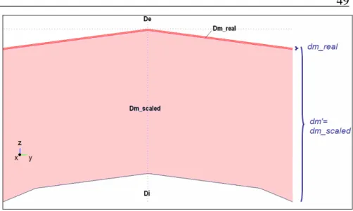
membrane, for model A. (Axis [m], Voltage [V]) ... 46 Fig. 17 Sketch of the modeled neurostimulation system (when only the axon segment is taken into account)... 48 Fig. 18 Zoom at the top of the implemented membrane domain: visual
VI
comparison (in plane y-z) between the real value of the membrane domain thickness dm_real and the actually implemented scaled one dm’
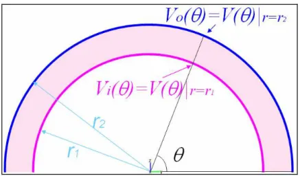
... 49 Fig. 19 Definition of inner and outer potential Vo and Vi for extrusion
... 52 Fig. 20 Input voltage waveform ... 54 Fig. 21 Correct underthreshold behaviour of the axon. Colormap: Vm [mV] at t=1.4ms, near the time in which the maximum voltage is reached. In red current density flux lines ... 54 Fig. 22 Vm(t) [mV] vs t[ms]. Understimulation: only electrotonic passive response ... 55 Fig. 23 Correct overthreshold behaviour of the axon. Vm [mV] at
t=0.525ms, near the time in which the maximum voltage is reached.
In red current density flux lines... 56 Fig. 24 Elicited AP in correspondence of a point 2.5µm translated along x from the projection of the nanoelectrode on the axon.
Vm[mV], t[ms]... 56
Fig. 25 Pink (Vm(t)[mV] vs t[ms]): two APs elicited (the second lower in amplitude as expected). Blue: input voltage stress... 57 Fig. 26 Two nearer pulsed (blue) elicit only one AP: Vm(t)[mV] vs t[ms] (pink). The second peak is an electrotonic potential... 57 Fig. 27 APs (Vm(t) [mV] , t[ms]).
∆
t is the delay between two pointsshifted by a couple of microns... 58 Fig. 28 From up to down, structure at t=0.5ms, t= 0.78ms, t=0.98ms: colormap Vm [mV]. Moving active zones (fluxes lines of current density in red) ... 59 Fig. 29 Sketch of the modeled neurostimulation system when the neuron is stimulated in proximity of the soma( axes are in µm) ... 60 Fig. 30 Piece of the transversal section (in plane x-z) of the model depicted in Fig. 29. Different sections are highlighted whose union constitutes membrane domain Dm. Inner Vi(x,y,z) (pink) and outer voltage Vo(x,y,z) (blue) ... 61 Fig. 31 Sketch of the rototranslated axis to define axon hillock
variables and to perform extrusion along normal direction to the axon hillock membrane domain (pink) ... 70 Fig. 32 Sketch of the rototranslated axis [X3 Y3 Z3]to define junction section variables and to perform extrusion from boundary delimiting the bottom of Dm_j domain (whose section in plane x-z is colored in
VII
Fig. 33 Understhreshold expected behaviour Vm[mV]. No active zone
... 75
Fig. 34 Vm(t)[mV] vs t[ms].Underthreshold correct behaviour... 75
Fig. 35 Overthreshold behaviour. Colormap: Vm [mV]. Red fluxes lines : current density ... 76
Fig. 36 Transmembrane voltage Vm(t) [mV], t[ms] ... 76
Fig. 37 Propagative effect: colormap of TMV [mV] at a) t=1ms and b) t=1.5ms... 77
Fig. 38 Very narrow AP (Vm[mV] vs t[s]) elicitation due to a triangular waveform. As expected when the stimulus is very strong a block of the action potential generation occurs... 78
Fig. 39 Figure extracted from [46] ... 78
Fig. 40 Overthreshold behaviour. Colormap TMV [mV]. Input stress: symmetric triangular waveform (peak amplitude -100mV, absolute value of slope 200V/s)... 80
Fig. 41 Comparison between the two different TMVs Vm1(t) and Vm2(t) [mV] vs t[s] (@ point of coordinates (2.88µm,0,0.72µm). simulated with MODEL1 (with membrane- magenta) and MODEL2 (with thin layer approximation-blue) ... 81
Fig. 42 Relative error of the Vm [mV] vs t[s]: only in a very few points there is a significant difference between the the two models predictions, thus leading to an RMSE of almost 4mV... 82
Fig. 43 Vm(t) [mV] vs t[s] according to MODEL1 (magenta) and MODEL2 (blue) ... 83
Fig. 44 Relative error on the calculation of Vm(t) vs t[s]... 84
Fig. 45 Ps are triggered on both axons: no selectivity obtained. Color map:Vm [mV]. Fluxes lines in red: current density entering also the second neuron are sufficient to elicit an AP also in the latter ... 86
Fig. 46 TMV [mV] vs t[ms], evaluated across the membranes of the two axons. Vm(t) in the target cell (green) and in the “victim” cell (blue) ... 87
Fig. 47 Schematic diagram of an elaborated advanced numerical prototyping algorithm [59]. ... 89
Fig. 48 A schematic representation of experiments main features and applications for the DoE technique [60] ... 90
Fig. 49 Notation for the 3k Design... 94
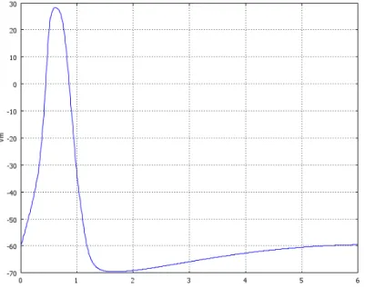
Fig. 50 Definition of tth... 98
Fig. 51 Time shape of Vin(t) ... 99 Fig. 52 Plane y-z: a simulated particular stimulation condition for the
VIII
geometrical parameters, reproduced as an example to graphically
represent Dy, r and ln and d(axis values are expressed in µm) ... 100
Fig. 53 Dex scatter plot representing PF values when a variable is fixed to its extreme values (minimum and maximum), while the others are free to vary... 103
Fig. 54 Number of triggered APs when each parameter is at its minimum (blue) or maximum (pink)... 104
Fig. 55 Dex scatter plot for tth PF [s] ... 105
Fig. 56 Linear prediction plot t_th (measurement units: 0.1ms) ... 106
Fig. 57 Quadratic prediction plot tth [0.1ms] ... 108
Fig. 58 Response surface as deduced by quadratic regression model for tth [s] ... 109
Fig. 59 Definition of PF w... 111
Fig. 60 Quadratic prediction of the PF w (measurement units: 0.1ms) ... 112
Fig. 61 Response surface as deduced by quadratic regression model for w[s]... 113
Fig. 62 Dex scatter plot for VmM PF [mV]... 114
Fig. 63 Linear prediction plot for VmM at the optimum solution[mV] ... 115
Fig. 64 Example figure with an activated AP under the electrode (TMV is higher toward the red color) used to show parameters definition: Dx, ln... 117
Fig. 65 Dex scatter plot for VmM PF [mV] in the case of a stimulation near the soma ... 118
Fig. 66 Linear prediction plot for VmM at parameters best solution[mV]... 119
Fig. 67 Dex scatter plot for Vm2M PF [mV] ... 121
Fig. 68 Linear prediction plot for VmM at parameters best solution[mV]... 122
Chapter 1
Introduction
1.1
Interest of the matter
Computational modelling and analysis in biology and medicine have received major attention in recent years. The interdisciplinary efforts developed so far aimed at elucidating structures and functions of living systems with major challenges in computational modelling and analysis to understand, analyze and predict the complex mechanisms of biological systems. Continued research investigations in computational biology and physiology have addressed important issues across many applications spanning from molecular dynamics, biological signalling pathways, cellular biology and communication, tissue mechano-biology, organ function and performance, systemic auto regulation, all the way up to lifestyle and environmental influences and behavioural responses. Researchers are now beginning to address the grand challenge of multi-scale computational modelling and analysis: effectively capturing biological and physiological interdependencies across multiple observational scales –not only in time and space, but also in physiochemical modality– and doing so in a computationally efficient manner. The development of many such models involves the design of multimodal data acquisition instrumentation and systems capable of measuring and monitoring of structural and functional properties in vivo and in minimally invasive manner [1],[2]. Over the last few years, the research work is being extended not only to further improve the basic understanding of biological and physiological models but also to explore translational biomedical research. For example, multi-scale and multi-modal modelling approaches are now paving the way to better understanding of the mechanisms of disease and its treatment, thus helping to
establish diagnostic biomarkers, physiology-based patient selection criteria, and more principled strategies for choosing, personalizing and optimizing therapeutic options.
Multi-scale computational modelling [3] promises to become a fundamental contributor to future biomedical sciences and technologies, and personalised predictive healthcare.
In particular, current and emerging neural prostheses and therapies based on nerve stimulation and recording involve electrodes chronically interfaced to the central and peripheral nervous systems.[4]-[11] Applications include theoretical understanding on how networks of neurons develop over time and change in response to stimuli. Because of the interest in this field, many scientific studies have been carried out of neural development and plasticity focus on the spatiotemporal dynamics of neural activity.
Although neurons are complex electrochemical systems, they encode a large portion of the information that they process in quick voltage transients, known as action potentials (APs) [12]; thus, the ability to accurately measure the effects of stimulating and recording neural tissue main activities is essential to many scientific and engineering efforts.
From a much more practical point of view, other applications include upper and lower limb prostheses for spinal cord injury [13] and stroke; bladder prostheses, cochlear and brain-stem auditory prostheses, cortical recording for cognitive control of assistive devices [10], vagus nerve stimulation for epilepsy and depression and deep brain stimulation (DBS) ([14]-[17]) for essential tremor, Parkinson’s disease, epilepsy, dystonia or depression, as well as the design of biosensors for research aims and retinal and cortical visual prostheses.
All these research fields strongly require electrodes characterized by low impedance for recording or safe reversible charge injection for stimulation.
In particular, as far as retinal prosthetics are concerned, since photoreceptors may degenerate or cease to exist, as in age-related macular degeneration (AMD) and in retinitis pigmentosa (RP), leading to partial or complete blindness, great effort in research field([18],[27]), indeed, has been taken in the last years to tailor devices, capable of partly restoring sight, bypassing the
photoreceptors retinal layer[28].
There are two main approaches to retinal implants currently being studied by scientists across the globe; subretinal and epiretinal [29]. The subretinal approach [19],[24],[30] involves implanting the chip underneath the retina, specifically in the macular region. In this case, the macular region is believed to be the ideal location because this is the most sensitive area, which is responsible for producing clear images in sighted people. Instead, the epiretinal approach involves placing the chip on top of the macular region of the retina and requires additional equipment—like cameras or special glasses—to properly function.
Therefore, while subretinal prosthesis relay signals to the bipolar cells, epiretinal ones pass them directly to the ganglion cells, in turn, carrying them to specific brain areas for elaboration.
Focalizing on this latter case, passing through various stages of development, since the 70s-80s, plenty of studies have been conducted on arrays of microelectrodes (MEAs) [4],[30], for interfacing with the Central Nervous System (CNS) in general and with retina, in particular. Nevertheless, because of this technology intrinsic limitations (large size of the electrodes, causing pour spatial resolution, lack of control on the local electrical and chemical activity of axons and their neurotransmitters as well as the open-loop nature of the stimulation), new solutions have been sought and have emerged recently, thanks to the ongoing development of nanotechnology [1],[31]-[38].
In addition to this, for further improving retinal stimulation effectiveness, other constraints must be taken into account, concerning its main electrophysiological features.
Since as we will briefly discuss in Chapter 2, retina performs an encoding (compression) of images to fit the limited capacity of the optic nerve and this is necessary since there are almost one hundred times more photoreceptors than ganglion cells. Indeed, in correspondence with fovea (retinal area responsible for sharp central vision, necessary for any activity where visual detail is strongly required) there are relatively few ganglion cells, leading APs to brain areas through their axons (Fig. 1).
Moreover, an increase in stimulation intensity does not proportionally change the intensity of the singular AP (which depends
non linearly by various parameters), but it is, instead, translated into an increase in the number of transmitted pulses per unit of time
(all-or-nothing axon response, frequency codification).
This implies that, especially in epiretinal stimulation devices, the primary goals are multiple.
First of all they can be identified in gaining axon spatial selectivity [39], as well as in the ability to elicit APs as readily as possible: in response to a change of the visual scenario the coded information the neuron has to carry to the brain changes and thus the ideal triggering should be as prompt as possible, because instead information distortion can be generated.
This objective is, in turn, in trade-off with the other fundamental aim: the respect of axonal refractory periods, which prevent, after a first AP elicitation, a further excitation stimuli to be effective in producing new APs. Thus, it is clear how, especially in ganglion axons stimulation, in order to reduce information distortion, it is of paramount importance to accurately (and possibly systematically) investigate the effectiveness that the excitation instrumentation gains when it is interfaced with the cells. In literature, indeed, as we have seen, many investigations can be found differently addressing the topic of the neurostimulation and its effectiveness but less is done to precisely evaluate nanoscale effects (the system has intrinsically high nonlinearities thus severe reduction in some of its geometrical parameters -nanoelectrode vs microelectrode- are likely to lead to different system responses) or to approach the topic from a more analytical/systematic point of view.
1.2
Finite Element modelling and sensitivity
analysis on the neurostimulating system
This thesis is focussed on the description of the main results obtained applying Design of Experiment procedures on Finite Element Method (FEM) models, on purpose implemented, of a simple neurostimulating nanoelectrode system. Thus particular focus is cast on the description of the activity devoted to obtain the model tools on which to perform the investigations and on the study of the system performances.Furthermore, the nanoelectrode system is thought as a constitutive part of a nanoporous alumina (biocompatible) layer supporting the growth of nanoelectrodes, realizable with a bundle of MWCNTs, in interface with neural cells.
The implemented models are, indeed, different, depending on the neuron or system most prominent feature that was necessary to highlight and observe.
In particular, once defined the desired performance functions of the system (the elicitation of the APs, the speed at which this phenomenon starts when it starts, the space resolution of the neurostimulating stress), Response Surface Methodology (within the theoretical context of the Design of Experiments) is exploited to deduce particularly meaningful information on the system dynamics and on the most significant factors leading them.
The 3D FEM models range from a “nanostimulated” axon segment, to a whole complex structure constituted by soma, axon hillock and the very first segment of the departing axon, built in order to evaluate geometrical parameters and ionic channels distributions affecting APs activation. In the end, a system made up of a couple of axons is implemented to obtain a tool where it is possible to verify the space resolution (space selectivity among fibres) gained in the neurostimulation performed.
Chapter 2
A brief review on retina and neuron
electrophysiology
The retina in vertebrates is a light sensitive tissue covering the inner surface of the eye. The optical properties characterizing the eye are capable of creating an image of the on the retina, operating as the film in a camera. As previously said, when the light strikes this tissue, it initiates a sequence of chemical and electrical events that end by activating nerve impulses. Optic nerve then sends them to various visual centers of the brain, by means of the fibers it contains. Since during the embryonic development the retina and the optic nerve originate as outgrowths of the developing brain, retina is considered part of the central nervous system (CNS), constituting the only part of it that can be visualized in a non-invasive manner. The structure of this tissue is a complex superimposition of several layers of neurons interconnected by synapses. However, the only neurons directly sensitive to light are the photoreceptor cells: they can be classified in two subtypes, rods and cones. The first one work mainly in dim light and provide black-and-white vision, while cones are the main actors in daytime vision and in the perception of colours. The cones respond to bright light and mediate high-resolution colour vision during daylight illumination (also called "photopic" vision). The rods are saturated at daylight levels and don't contribute to pattern vision. However, rods do respond to dim light and mediate lower-resolution, monochromatic vision under very low levels of illumination (called "scotopic" vision), There is also another, less common type of photoreceptor, the photosentitive ganglion cell, which is important for reflexive responses to bright daylight. Neural signals from the rods and cones undergo a complex processing sequence by other neurons belonging to the retina itself . The output is in the form of APs in retinal ganglion cells axons. Several important features of visual perception can be
traced to the retinal encoding and processing of light.
2.1
Anatomy of vertebrate retina
Fig. 1 Section of retina. [40]
From innermost to outermost, the ten retinal layers include: • Inner limiting membrane - Müller cell footplates
• Nerve fiber layer - Essentially the axons of the ganglion cell nuclei.
• Ganglion cell layer - Layer that contains nuclei of ganglion cells and gives rise to optic nerve fibers.
• Inner plexiform layer.
• Inner nuclear layer contains bipolar cells, which correspond to heat and touch sensory skin receptors, capable of transmitting signals to the spinal cord or its continuation, the medulla.
• Outer plexiform layer • Outer nuclear layer
segment portions of the photoreceptors from their cell nucleus. • Photoreceptor layer - Rods and Cones
• Retinal pigment epithelium
Of these the four main layers of the ten, from outside in: pigment epithelium, the photoreceptor layer, bipolar cells, and finally, the ganglion cell layer. Therefore, the optic nerve is less a nerve than a central tract, connecting the bipolars to the lateral geniculate body, a visual relay station in the diencephalon (the rear of the forebrain). In adult humans the entire retina is approximately 72% of a sphere about 22 mm in diameter. An area of the retina is the optic disc, sometimes known as "the blind spot" because it lacks photoreceptors. It appears as an oval white area of 3 mm². In the direction of the temples there is the macula. At its centre is the fovea, a pit most sensitive to light and responsible for our sharp central vision. Around the fovea extends the central retina for about 6 mm and then the peripheral retina. In section the retina is no more than 0.5mm thick. It has three layers of nerve cells and two of synapses, including the unique ribbon synapses. The optic nerve carries the ganglion cell axons to the brain and the blood vessels that open into the retina. The ganglion cells lie innermost in the retina while the photoreceptive cells lie outermost. Because of this counter-intuitive arrangement, light must first pass through and around the ganglion cells and through the thickness of the retina, (including its capillary vessels) before reaching the rods and cones. However it does not pass through the epithelium or the choroid (both of which are opaque). Between the ganglion cell layer and the rods and cones there are two layers of neuropils where synaptic contacts are made. The neuropil layers are the outer plexiform layer and the inner plexiform layer. In the outer the rods and cones connect to the vertically running bipolar cells, and the (horizontally oriented) horizontal cells connect to ganglion cells. The central retina is cone-dominated and the peripheral retina is rod-cone-dominated. In the central macular fovea zone the cones are smallest and arranged in a hexagonal mosaic, the most efficient and highest density.The area directly surrounding the fovea has the highest density of rods converging on single bipolars. Since the cones have a much lesser power of merging signals, the fovea allows for the sharpest vision the eye can attain .Since, as we said there are much more receptors than optic nerve fibers, and the horizontal action of the horizontal and
amacrine cells can allow one area of the retina to control another (e.g., one stimulus inhibiting another), the messages are merged and mixed. An image is produced by the "patterned excitation" of the cones and rods in the retina. The information retina sends is processed by the neuronal system and various parts of the brain working in parallel to form a representation of the external environment. The response of cones to various wavelengths of light is called their “spectral sensitivity”. In normal human vision, the spectral sensitivity of a cone falls into one of three subgroups. These are often called "red, green, and blue" cones but more accurately are short, medium, and long wavelength sensitive cone subgroups. When light falls on a receptor it sends a proportional response synaptically to bipolar cells which in turn signal the retinal ganglion cells. The receptors are also 'cross-linked' by horizontal cells and amacrine cells, which modify the synaptic signal before the ganglion cells. In the retinal ganglion cells there are two types of response, depending on the receptive field of the cell. Since there are more retinal receptors, than axons in the optic nerve; a large amount of pre-processing is performed within the retina. The fovea produces the most accurate information. Despite occupying about 0.01% of the visual field (less than 2° of visual angle), about 10% of axons in the optic nerve are devoted to the fovea. The resolution limit of the fovea has been determined at around 10,000 points. The information capacity is estimated at 500,000 bits per second without colour or around 600,000 bits per second including colour. The retina, unlike a camera, does not simply send a picture to the brain. It spatially encodes (compresses) the image to fit the limited capacity of the optic nerve. We remind that compression is necessary because there are 100 times more photoreceptors cells than ganglion cells as mentioned above. The retina does so by "decorrelating" the incoming images. These operations are carried out by the center surround structures as implemented by the bipolar and ganglion cells. Finally, the horizontal and amacrine cells play a significant role in this process. Once the image is spatially encoded by the center surround structures, the signal is sent out the optical nerve (via the axons of the ganglion cells) through the optic chiasm to the LGN (lateral geniculate nucleus) and then to the V1 Primary visual cortex.
2.2
Anatomy of vertebrate retina: the nervous
cell
The nerve cell [41] can be divided into four different zones in terms of morphological features: cell body (soma), dendrites, axon and presynaptic axon terminals, each playing a particular role in the genesis of nerve signals. The cell body (soma) is the metabolic center of the neuron, gives rise to two types of extensions, axon and dendrites, which branch off as a harborization from the cell body and the human body apparatus are intended to receive the messages arriving to the neuron from other nerve cells The cell body also gives rise to the axon is a cylindrical process, with a diameter (in humans) from 0.2 to 20 µm. It is also capable of transmitting information over long distances by propagating an electrical signal of all-or-nothing of very short duration, called indeed the Action Potential; it is the major route of conduction of the signals of the neuron. Once the transmembrane voltage has reached the critical threshold, an AP is typically generated at a specialized area where the axon originates, the axon hillock. The axon is divided into many thin branches, each of which has specialized swellings, called presynaptic terminations, which are the support for messages transmission.
Fig. 2 The nervous cell
It is through these terminals that neurons transmit information about its activities at the interfaces of other neurons (dendrites and cell
bodies). The “contact” points are called synapses and therefore the cell that transmits the information is that the presynaptic cell, while the receiving is called postsynaptic. Between the two there is a space called the synaptic cleft, which communicates freely with the extracellular space. Most of the presynaptic neurons finish close to the postsynaptic dendrites of the neuron but contact between neurons can be sometimes with the soma or, less frequently, with axon initial or terminal segment.
Chapter 3
Modelling of the Neurostimulation
System
3.1
Neurostimulation system issues and choices
Carbon nanotubes are attractive as neural electrodes because of a very wide range of reasons. A very high Electrical Superficial Area / Geometrical Superficial Area ratio, (ESA/GSA), is inherent in the nanotube geometry, which gives rise to a large double-layer charge capacity; for neural stimulation: in literature charge-injection capacities have been found of 1–1.6 mC cm−2 with vertically aligned nanotube electrodes. Works on the development of nanotube and nanofibre neural interfaces have been reported, as introduced in Chapter 1. The discovered excellent biocompatibility of carbon nanotubes, especially with CNS, [42]-[44], has paved the way for deeper investigation into the possibility of using them to improve microelectrode performances or even to obtain nanoelectrodes. Moreover, microelectrodes coated with CNTs have been proposed [36] , in order to obtain a rougher surface, providing a better electrical coupling with the cells. Furthermore, thanks to their additional properties (high mechanical resistance and electrical conductivity, extremely small diameters, good experienced Signal-to-Noise-Ratio and capability to be functionalized and to be used as neurotransmitters sensors), CNTs have been suggested as strongly efficient nanoelectrodes [31]-[38].The resulting advantages are clearly understood: tri-modal Nanoelectrode Arrays (NEA) have been investigated in [33], allowing much higher spatial resolution for the electrical stimulation and capability of recording and monitoring of neurotransmitters levels (closed-loop control). Carbon nanotubes may also be chemically modified to enhance biocompatibility or provideother functional properties (they are even investigated in literature as anticorrosive coating agents for general purpose metallic electrodes [45]).Their usage, thus, deeply favours quantitative improvement of the neurostimulating apparatus and outperforms the metallic more corruptible metallic electrodes.
These are the reasons why we have chosen to investigate the properties of a system realizable with CNT based nanoelectrodes.
Another particularly meaningful issue to decide for has been the type of modelling approach.
3.1.1
The necessity of a modeling approach
Keeping in mind the objective of this work, it is clear that it is of paramount importance to develop an accurate mathematical model to the entire system. We are moving within the field of virtual engineering (specifically applying DoE- Design of Experiments- techniques), in order to benefit of all its advantages. In particular, virtual engineering integrates geometric models and related engineering tools such as analysis, simulation, eventual optimization and decision making tools, etc., within a computer-generated environment that facilitates multidisciplinary product development. This requires a model that includes the geometry, physics, and any quantitative or qualitative data from the real system, so that is possible to observe how it works and how it responds to changes in design, operation or any other engineering modification. A model requires selecting and identifying relevant aspects of a situation in the real world and exploits mathematical language. In this way, the real system can be analyzed, in order to be controlled or optimized, using the mathematical model to take into account its peculiar and most meaningful features and to try to estimate how an unforeseeable event could affect it. The system is described by a set of variables and of equations that establish relationships between the variables, representing some properties of the system, for example, signals or events occurrence. The actual model is the set of functions that describe the relations between the different variables, classifiable as decision, input, state, exogenous, random and output variables. Different system constraints and objective functions (also called indexes of performance) can be identified whose interest strongly
depends on the specific application. Mathematical models can be classified in linear (or nonlinear), deterministic (or stochastic), static (or dynamic). In general, model complexity involves a trade-off between simplicity and accuracy. Occam's Razor is a principle particularly relevant to modelling; the essential idea being that among models with roughly equal predictive power, the simplest one is the most desirable. While added complexity usually improves the realism of a model, it can make it difficult to understand and analyze, and can also pose computational problems, including numerical instability.
3.1.2
The field solution and the Finite Element Method
adoption
As far as this thesis work is concerned, our choice has been to model the reality under study by means of a nonlinear, deterministic and dynamic model, taking into account the nature of the reality to emulate. In particular, it has been necessary to decide which was the best modelling technique to capture the main features of the problem under analysis. We have opted for a field solution model and the Finite Element Method to implement it. Very often in literature the matter is addressed by using biomolecular or compartmental approaches .[3],[46]-[48]. Indeed, it is very difficult to (e.g.) “tailor” appropriate density fluxes lines for currents or electric field lines or analyzing systematically different electrode configurations, adopting biomolecular or compartmental typical modelling solutions. The first one has a much deeper and detailed breath than what is necessary for our investigation: it is focused more on the study of proteins, properties of enzymes, metabolic pathways, than on their interactions with the applied electric fields and the higher scale phenomena related, making it very uneasy to explore the performances we wanted to explore. For the second classically used model, the compartmental, it must be said that one of its big disadvantages (evidenced in many models used so far) is that on the one hand it is not possible to simulate the interaction between activated fibres and the surrounding tissue (making the implemented models less extensible and thus less useful), on the other hand it is very difficult to integrate geometrical aspects and time dependency.
Thus, within this thesis work, our choice has fallen on the field solution (which has started to be more appreciated in the last years also thanks to greater power of calculus), because it allows to overcome all the cited troubles, especially in the flexible and manageable FEM implementation [8]. We are, thus, enabled to couple, quite simply, multiphysical parameters and descriptive equations into a whole system and to have the opportunity to quite easily make parametric geometrical variations and adaptations.
In the end, our modelling of neuron membrane highly nonlinear behaviour has been based on the set of equations that the two Nobel Prizes, A. L. Hodgkin and A. F. Huxley, published [49], paving the way for the research in the field. Their mathematical theory on neural membrane electrophysiology uncovered the gating mechanisms in axons and represents a milestone in understanding and modelling the excitation and spike propagation in nerve and muscle fibres. Therefore it is by far the most broadly adopted in literature to simulate neural activities [12]. These equations, indeed, once coupled with Maxwell equations for electromagnetic fields, represent the suitable tool for describing sufficiently accurately neuron response to nanoelectrode stimulation. In particular, since the typical frequencies involved in neural stimulation are quite low, their quasi static formulation has been adopted. Finally, in the next subsection a brief overview of the Finite Element Method is reported to better clarify its advantages and the reasons of its choice, while the subsequent sections of the chapter follow the modelling phases. Once obtained the 2D representation of the main axon features, we have proceeded (following a a step by step procedure) towards the implementation of a valid 3D model tool, which is supposed to take into account more sophisticated and spatially differentiated neuron operating conditions. 3.1.2.1Notes on the theory of FEM
The finite element method (FEM) is a very widely adopted numerical technique employed to obtain approximate solutions to partial differential equations (PDE) and to integral ones. Euler’s and Runge-Kutta method together with other standard techniques are used to perform numerical integration for solving the ordinary differential system of equations (ODE) in which the PDE are approximated.
Indeed, in this context, the primary goal is to determine equations that approximate those under study, with the constraint of a good numerical stability. This means that errors in the input and in the intermediate calculations phases should not accumulate, causing the resulting output to be less meaningful or meaningless at all. In literature there are various possible techniques, but FEM is a good choice for solving partial differential equations over complicated or time changing domains, when the desired precision varies over the entire domain or when the solution lacks smoothness. This paragraph very briefly describes how the FEM approximates the PDE problem with a problem that has a finite number of unknown parameters, leading to a discretization of the original problem. To do so an introduction must be done to finite elements and shape functions, that describe the possible forms of the approximate solution.
The starting point for the finite element method is a mesh, a partition of the geometry into small units of a simple shape: mesh elements. Different types of elements are available in 1D, 2D, and 3D. Sometimes the term “mesh element” means any of the mesh elements—mesh faces, mesh edges, or mesh vertices. In particular, mesh elements of a particular domain in the geometry (a subdomain, boundary, edge, or vertex) have its dimensionality: a d-dimensional domain is discretized with d-dimensional mesh elements (Fig. 3).
Once performed this first problem partitioning task, it is possible to introduce approximations to the dependent variables. An example is clarifying. Let us consider the case of a single variable.
Fig. 3 Geometry approximation by meshing
If we analyze it, from a basic point of view, the FEM solves equations in the matrix form, as synthesized in Fig. 4, where the analogy is reported with the mechanics terminology, form which it inherited the approach. Written in a very simple and intuitive form, what the solver
has to obtain at the end of all the geometrical problem discretizing and linearization , is the solution of a matrix equation in the form reported in Fig. 4., where u is the vector of the unknown values assumed by the dependent variable on the nodes of the discretized geometry. Attention must be paid to avoid situations like the one reported in Fig. 5 where there is a so called ill conditioning of the problem, since (keeping the analogy with elastic constants and mechanics) the two elastic constants (in general the elements of the stiffness matrix K) are extremely different in amplitude, thus posing computational problems.
Fig. 4 The philosophy and also terminology of FEM borrowed from the mechanics
In particular, the general idea is to approximate u with a function that it is possible to describe with a finite number of parameters, the so-called degrees of freedom (DOF). Inserting this approximation into the weak form (that we will later briefly discuss ) of the equation generates a system of equations for the degrees of freedom.
Fig. 5 Simple example of an ill conditioned problem
elements in 1D. Let us assume that a mesh consists of just two mesh intervals: 0 < x < 1 and 1 < x < 2. Linear elements means that on each mesh interval the continuous function u is linear (affine). Thus, the only thing there is need to know in order to characterize u uniquely is its values at the node points x1 = 0, x2 = 1, and x3 = 2. Denote these as U1 = u(0), U2 = u(1), U3 = u(2). These are the degrees of freedom.
Now it is possible to write:
) x ( U ) x ( U ) x ( U ) x ( u 2 2 3 3 1 1
ϕ
+ϕ
+ϕ
= (1)where
ϕ
i(x) are certain piecewise linear functions. Namely,ϕ
i(x) is the function that is linear on each mesh interval, equals 1 at the ith node point, and equals 0 at the other node points. For example, ≤ ≤ ≤ ≤ − = 2 0 1 x 1 ) x ( 1 x1 1 if x1 0 if
ϕ
(2)The
ϕ
i(x) are called the basis functions. The set of functions u(x) is a linear function space called the finite element space.For better accuracy, it is possible to consider other finite element spaces corresponding to quadratic, cubic, etc. elements. Functions u in this space are 2nd, 3rd, etc. polynomials on each mesh interval.
Moreover, in general, a finite element space is specified by giving a set of basis functions.
Fig. 6 An example showing the degree of approximation due to different orders of the elements
The description of the basis functions is, furtherly, simplified by the introduction of local coordinates (or element coordinates). Let us consider a d-dimensional mesh element in an n-dimensional geometry (whose space coordinates are denoted by x1,..., xn) and the standard
d-dimensional simplex: 1 ... , 0 ,..., 0 , 0 2 d 1 2 d 1 ≥
ξ
≥ξ
≥ξ
+ξ
+ξ
≤ξ
(3)which resides in the local coordinate space parametrized by the local coordinates ξ1, …, ξd. If d = 1, then this simplex is the unit interval. If
d = 2, it is a triangle with two 45 degree angles, and if d = 3 it is a
tetrahedron.
If we consider the mesh element as a linear transformation of the standard simplex, namely, by letting the global space coordinates
xi be suitable linear (affine) functions of the local coordinates, it is possible to get the mesh element as the image of the standard simplex; when described in terms of local coordinates, the basis functions assume one of a few basic shapes. These are the shape functions.
Moreover, when using higher-order elements (that is, elements of an order > 1), the solution has a smaller error. The error also depends on how well the mesh approximates the true boundary. To keep errors in the finite element approximation and the boundary approximation at the same level, it is wise to use curved mesh
elements. They are distorted mesh elements that can approximate a
boundary better than ordinary straight elements (if the boundary of the problem is curved). It is possible to get curved mesh elements by writing the global coordinates xi as polynomials of order k (the
geometry shape order) in the local coordinates ξj For mesh elements that do not touch the boundary, there is no reason to make them curved, so they are straight.
The order k is determined by choosing the geometry shape order for the coordinate system associated with the finite element.
Nevertheless, if a curved mesh element becomes too distorted, it can become inverted and cause problems in the solution. This is exactly what happens in one of the models described in the following sections. More details for the solution adopted for this inconvenient are indeed reported in § 3.3.2.2
In this brief overview, it must be pointed out that our choice for all the modeled structures has fallen on the Lagrange element type (piecewise polynomials of degree k). They are indeed widely used since they are available with all types of mesh elements.
mention the choice of the type of analysis (linear, non linear, time dependent non linear, etc.) strongly depending on the physical and mathematical features inherent the reality to model.
In general, the solvers break down each problem—whether linear or nonlinear—into one or several linear systems of equations by approximating the given problem with a linearized problem. The coefficient matrix of the discretized linearized problem is called the
Jacobian matrix (or stiffness matrix), just the one cited in the
introductory part of this paragraph. Moreover, since in this work we have used for all our models the time-dependent solver, it is necessary to highlight that it must be chosen (it is indeed the one we have used for all our investigations) to find the solution to linear or nonlinear
time-dependent PDE problems, also known as dynamic problems or unsteady problems.
Indeed, the general formulation of a time-dependent PDE (defined on computational domains in 1D, 2D, or 3D) in coefficient form is:
(
c u u)
u au f t u d t u e a 2 2 a + ∂∂ +∇⋅ − ∇ − + + ⋅∇ + = ∂ ∂ α γ β (4) where:• ea is called mass coefficient
• ea is said to be damping coefficient, or mass coefficient. • c is the diffusion coefficient.
• α is the conservative flux convection coefficient. • β is called the convection coefficient.
• a is the absorption coefficient.
• γ is the conservative flux source term. • f is the source term.
This PDE formulation together with boundary and initial conditions fully define the problem.
The time-dependent solver operates a discretization of the problem, leading to a differential-algebraic system (DAE) or to ordinary differential equations (ODE), solved by appropriately chosen algorithm. Thus the solver is an implicit time-stepping scheme, which implies that it must solve a possibly nonlinear system of equations at each time step. It solves the nonlinear system using a Newton
iteration, and it then solves the resulting systems with an arbitrary linear system solver.
Furthermore, it is sometimes essential for accuracy or performance to set absolute and relative tolerance parameters for the time-dependent solver. They are tolerances to control the error in each integration step. More specifically, let U be the solution vector corresponding to the solution at a certain time step, and let E be the solver estimate of the (local) error in U committed during this time step. The step is accepted if
1 N N 1 i 2 U R A E i i i <
∑
= + (5)where Ai is the absolute tolerance for DOF i, R is the relative tolerance, and N is the number of degrees of freedom. The accumulated (global) error can be larger than the sum of the local errors for all the integration steps. However, the solver’s error estimate is often too pessimistic, which means that the estimated local error typically is of the same order of magnitude as the true global error.
To conclude our brief digression on FEM, it is very useful to point out, as in some cases it has been used in modelling the neural cell structures that we will describe in the following sections, that there is an alternative formulation of the problem, different from the one defined in (4): it is the so-called weak formulation.
Indeed, eq. (4) is a strong definition, while the problem can be also solved working on the integral formulation (the weak one) of the PDE, using test functions. In the practice, they are adopted to multiply both members of eq. (4) and then integrate over the domain of interest to solve the problem in its integral definition. Thus, unlike the other formulation, the weak form takes on the character of generality, allowing greater flexibility in setting the conditions: it is possible to assign constraints on subdomains, boundaries , edges and points. Moreover, it is always possible to translate a strong formulation into the weak one, if the used test function is a well-behaved function,
while the converse is not always true. Moreover in the boundary weak
form, it is possible to solve for variables defined only on boundaries
and couple this equation with other equations defined on a subdomain. This technique is particularly useful in modelling adsorption processes (where it is necessary for balances on the edges to “agree” with those in adjacent domains) for a smart-handling of extremely thin layers. This will be clearly demonstrated in the next sections by the reduction in computational burden attained exploiting the well known technique of the thin layers approximation and validating the obtained results with a non-approximated model.
To summarize: modelling with FEM requires a preprocessing, the solving phase and the analysis of the results, proceeding following the reported steps:
1) Selection of the analysis type (transient dynamic analysis with time dependent solver is the one we use in this thesis work);
2) Selection of the element dimensionality and type, depending on the problem to solve and on the geometry analyzed (2-D, 3-D) leading to linear, quadratic, etc. elements;
3) Choice of the primary material properties to model; 4) Choice of nodes positioning;
5) Construction of the elements by assigning connectivity between the nodes (these last two are typically implemented automatically by an algorithm, in our case the Delaunay one);
6) Application of the boundary conditions and “input stresses”;
7) Processing: solution of the (eventually time-varying) boundary value problem;
3.2
Hodgkin-Huxley lumped circuit set of
differential equations translated into field
ones (2D case).
Fig. 7 The axon slice under analysis (3D sketch). The section in r-z plane is highlighted in pink
Here a description is performed of the FEM model For a nanoelectrode-axon segment stimulation system.
A 2D FEM model of the stimulating equipment and of the axon segment is implemented that simulates the most relevant dynamics of spatiotemporal transmembrane voltage (TMV) [50].
Bases on Hodgkin and Huxley (HH) set of highly non linear differential equations (linking the phenomena of chemical transport through the membrane with the electrical dynamics of the neuron), a translation is performed in terms of electromagnetic parameters in three dimensions. Coupling this model with the quasi-static formulation of Maxwell equations the elicitation and propagation of APs is obtained by exploiting the high nonlinearity of the medium membrane. Indeed, the nonlinearity of the membrane is not modelled as classically in literature by using the so-called "cable equation" which has the disadvantage of having to estimate in advance the speed of propagation of the AP along the axon, but is implemented "implicitly", using the definition itself of the equivalent conductivity which is gained by the translation itself of Hodgkin-Huxley equations suitable for a field solution.
The adopted modelling approach has been modular and incremental since, in order to have a first comparison with literature data, before starting with a three dimensional modelling activity, a 2D
accurate model has been realized, for a section of tubular segment of a nervous cell axon (the neuronal structure carrying nervous signals) which takes into account, through the so called Hodgkin-Huxley (HH) equations , the non linear and time varying behaviour of the membrane that surrounds it. The lumped-circuit quantities of the HH electrophysiological model are transformed into parameters adapt to a
field solution study. In fact, the Electro Quasi Static (EQS)
formulation of the Maxwell equations describing the relevant phenomena is faced by using the Finite Element Method (FEM). The non linear differential equations describing the membrane behaviour are efficiently and accurately combined with the FEM solution in a numerical procedure performed by using COMSOL Multiphysics®. The proposed procedure is then employed to evaluate the space and time dynamics of the Action Potential (AP) along the axon segment. Due to its simple implementation the proposed model can be easily used to simulate the behaviour of more complex nervous structures. The simulation procedure encompasses three phases: the first, in which the resting (static) solution is calculated, thus ensuring that the correct starting point for dynamic simulations is obtained, the second one, exploited to simulate non-propagated APs and the third one to reproduce their propagation along the segment under examination. The extrusion feature of COMSOL Multiphysics proves to be a very helpful tool in projecting variables (voltages) from cell membrane boundaries onto the domain itself, where the calculation of its voltage-dependent electric conductivity needs to be performed.
In addition, the very small dimension of the membrane thickness compared to the other geometrical dimensions of the system is approximated, in an alternative version of the model, as a thin layer thus leading to a sensible reduction of the computation burden. A comparison between the two model versions has led to very satisfactory results, as far as APs elicitation and propagation are concerned.
3.2.1
The extrusion tool in FEM modelling
In FE modeling an extrusion coupling variable maps values from a source domain to a destination domain. When the domains are of the same space dimension, and it is typically a point-wise mapping. When
the destination domain has higher dimension than the source one, the mapping is done by extruding point-wise values to the higher dimensions. It is possible to define the transformation between the source and destination in two ways: as a linear or a general
transformation.
The linear transformation maps between domains of the same dimension. The domains can exist in geometries of different space dimensions. For example, it is possible to couple from edges in 2D to those in 3D or 2D subdomains to 3D faces. In these cases obviously there is need of geometries of different space dimensions for the source and destination. The linear transformation is defined by specifying points in both the source and destination.
As far as the general transformation is concerned, instead, the extrusion coupling variable defines a more general transformation between source and destination than the linear one. Specifically, when the destination domain has more space dimensions than the source domain, the variable performs extrusion of values.
Fig. 8 Example of a general transformation mapping from a 2D to a 3D domain [51]
The definition of any extrusion coupling variable involves two mesh transformations, which are important to understand. The source
transformation is a one-to-one mapping that maps the mesh of the
physical source domain to an intermediate mesh embedded in a space of the same dimension as the source. The destination transformation is a mapping from the destination domain, where the value of the variable is defined, to the same space that contains the intermediate mesh.When the value is requested of the coupling variable somewhere in the destination domain, the transformation of the destination points is realized, using the destination transformation. It compares the resulting coordinates to the elements in the intermediate mesh to find corresponding locations in the physical source domain. This means that the source transformation must be inverted but not the destination transformation. The latter can in fact be noninvertible, which is, for example, the case for a linear extrusion.
To avoid the need to solve a nonlinear system of equations for every destination point, the software solver assumes that the source transformation is linear on each element of the intermediate mesh. In practice, the transformation is often trivial and leaves the coordinates unchanged, but it can also rescale, stretch, bend, or reflect the mesh. It is important to notice that the definition must be performed of the source transformation that maps the source domain to the intermediate domain of the same dimension. The source transformation has the
same number of fields as the dimension of the source domain.
Expressions can be used containing space coordinates in the source geometry when defining the transformation. It is moreover necessary to highlight that the transformation must be approximately linear within each mesh element. When defining the transformation it is, also, permissible to use expressions containing space coordinates in the destination geometry and specifying an arbitrary transformation, which can be highly nonlinear or noninvertible.
To summarize the general case, we can say that if source and destination transformation are defined according to Table 1, the FEM solver operates a back substitution starting from the destination domain D.
Table 1 Extrusion general transformation in the most general form: when the source domain is 3D
Source Transformation Destination Transformation
= = = ) z , y , x ( S Z ) z , y , x ( S Y ) z , y , x ( S X z src y src x src = = = ) z , y , x ( S Z ) z , y , x ( D Y ) z , y , x ( D X z dest y dest x dest
Here the final goal, in extruding the assigned variable Var from the source domain S to D, is to calculate its value in every point
Pi(xi,yi,zi), belonging to the destination domain mesh. In order to do so, it is necessary for the solver to determine, once given Pi which are the coordinates (xj,yj,zj) of the corresponding point Pj(xj,yj,zj) in S, where Var(Pi)=Var(Pj). In particular, going through the following series of passages for every assigned point Pi(xi,yi,zi), the solver firstly determines Xdest, Ydest and Zdest (this way destination transformation can be also non invertible) (6) and then matches them with the values of Xsrc , Ysrc and Zsrc respectively (7). = = = = = = * Z ) z , y , x ( D Z * Y ) z , y , x ( D Y * X ) z , y , x ( D X i i i P z dest P y dest P x dest (6) = = = dest src dest src dest src Z Z Y Y X X (7)
Now, since source transformation must be invertible the coordinates can be finally determined of the point Pj(xj,yj,zj) as in (8), obviously including as third equation (there are three d.o.f.) the geometrical constraint assuring Pj to belongs to the its particular subdomain


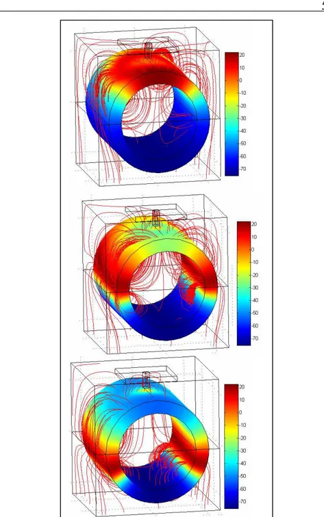
![Fig. 15 Propagation phenomenon: the moving active zone. Potential map at three different times of pulse conduction (Axes [m], Voltage [V])__](https://thumb-eu.123doks.com/thumbv2/123dokorg/7204971.76004/57.892.106.623.214.1017/propagation-phenomenon-moving-active-potential-different-conduction-voltage.webp)
![Fig. 16 a) Simulation results for local currents in an activated zone compared with literature behaviour in the inset [56]](https://thumb-eu.123doks.com/thumbv2/123dokorg/7204971.76004/58.892.275.780.208.773/simulation-results-local-currents-activated-compared-literature-behaviour.webp)
![Fig. 26 Two nearer pulsed (blue) elicit only one AP: V m (t) [mV] vs t[ms] (pink). The second peak is an electrotonic potential](https://thumb-eu.123doks.com/thumbv2/123dokorg/7204971.76004/69.892.129.589.658.968/fig-nearer-pulsed-elicit-pink-second-electrotonic-potential.webp)
![Fig. 27 APs (Vm(t) [mV] , t[ms]). ∆∆∆∆ t is the delay between two points shifted by a couple of microns](https://thumb-eu.123doks.com/thumbv2/123dokorg/7204971.76004/70.892.318.744.439.723/fig-aps-vm-delay-points-shifted-couple-microns.webp)