Chapter 2 Comprehensive model for NO emissions in MILD combustion lab-scale burner

Comprehensive model for NO

emissions in MILD combustion

lab-scale burner

This present Chapter describes the development of a new comprehensive model for NO formation in MILD regime, such as Jet in Hot Coflow (JHC) burner. The model has been tested under different conditions through numerical simulations, in order to provide a better estimations of such pollutant.

2.1 Description of JHC burner

The peculiarity of Jet in Hot Coflow burner is that it operates in the so-called Moderate or Intense Low-oxygen Dilution (MILD) combustion regime [24], which ensures high combustion efficiency with low NOx emissions, as expressed in

Sec-tion 1.3.1. MILD combusSec-tion occurs when reactants are preheated above their self-ignition temperature and when enough inert are entrained in the reaction region to dilute the flame. As a result, a flame front is no longer identifiable (Flameless combustion). In comparison with conventional diffusion or premixed combustion regimes, volumetric enlargement of the reaction zone and more uniform tempera-ture distribution are unique featempera-tures of MILD combustion. MILD combustion is characterized by a strong coupling between turbulence and chemistry, occurring at similar timescales, so they should be treated with finite scale approaches [30]. Because of both the low-temperature conditions and the eventually presence of H2

characterizing MILD combustion, the thermal NO route becomes less significant, therefore other routes, such as N2O/NO and NNH route should be included, as

approximately, 30% energy savings and hence CO2 reduction [31].

Sabia et al. [32] reported that MILD combustion is a promising technology for low-calorific fuels, high-calorific industrial wastes as well as in presence of hydrogen. Derudi et al. [33] suggested MILD combustion for the utilization in the coke oven gas (COG), which is a by-product of the coke-making process. The use of MILD combustion is also foreseen for gas turbine applications [34], as its stable and noiseless characteristics may avoid the thermo-acoustic instabilities and stresses observed with conventional combustion.

Among the available experimental data on MILD combustion, the JHC burner experiment carried out by Dally et al. [35] has received many attentions because of the number and accuracy of experimental data. The fully characterized mean and fluctuating temperature and species fields for different oxygen levels (3%, 6% and 9%) in the hot coflow stream resulted in a number of publications aiming at the validation of different numerical approaches [36]-[40].

The unconfined JHC flames are complicated in that the turbulent flow field is dependent not only on mixing of three streams of different turbulence levels, but also on the flame cooling, weakened reaction zone and lower reaction rates. Such complex flames demand an accurate resolving of mixing and flow fields as a prerequisite to reasonably predict major and minor combustion products in sub-sequent steps. The JHC burner (Figure 2.1a) consists of an insultated and cooled

the combustion process. After a preliminary theoretical investigation of the EDC model and its sensitivity to the two model constants, the authors showed that the prediction of DJHC flames could be improved by changing these constants with respect to the classical EDC.

In the present paper, the structure of JHC burner experimentally studied by Dally

et al. [25] is investigated using the steady state Reynolds-Averaged Navier-Stokes

approach coupled with the Eddy Dissipation Concept for the turbulence-chemistry interaction treatment. An analysis of the EDC model to improve its predictions for MILD combustion conditions is presented in the last section.

2 Test Case

The jet-in-hot coflow burner modeled in this work has been experimentally studied

by Dally et al. [25] and is shown in Fig. 1. It consists of a fuel jet nozzle, which has

an inner diameter of 4.25 mm and a wall thickness of 0.2 mm, located at the center of a perforated disc in an annulus, with inner diameter of 82 mm and wall thickness of 2.8 mm, which provides nearly uniform composition of hot oxidizer coflow to the reaction zone. The entire burner was sited inside a wind tunnel introducing room

temperature air at the same velocity as the hot coflow. Table1shows the operating

conditions of three inlet streams for the different case studies. The notations, HM1, HM2 and HM3, refer to the flames with oxygen mass fraction of 3%, 6%, and 9%, respectively, in the hot coflow stream. The jet Reynolds number was around 10000 for all flames. The available data consist of the mean and root mean square (rms) of

temperature and concentration of major (CH4, H2, H2O, CO2, N2and O2)and minor

species (NO, CO and OH).

2.125mm 41mm 120mm z r 900mm 100mm Upstream Downstream Center of fuel jet nozzle (0,0) Tunnel air Hot coflow Fuel jet

(b)

(a)

Fig. 1 (a) Schematic of the jet-in-hot coflow burner [25] and (b) computational domain with

boundary conditions

(a) (b)

central jet, which has an inner diameter of 4.25 mm and a wall thickness of 0.2 mm, through which a hybrid fuel of methane and hydrogen (88% and 12% respectively, as mass fraction) is injected with Reynolds number of 10,000 to the hot oxidizer. The ject is located at the center of a perforated disc in an annulus, with inner diameter of 82 mm and wall thickness of 2.8 mm, which provides nearly uniform composition of hot oxidizer coflow to the reaction zone. The entire burner was sited inside a wind tunnel, which provided room temperature air at the same velocity as the hot coflow. It can operate at a wide range of coflow temperatures and O2

levels.

Table 2.1: Operating conditions for cases studied (compositions are as mass fractions)[40]

Fuel jet (CH4/H2) Oxidant coflow

Case T (K) Re u(m/s) T (K) O2(%) N2(%) H2O(%) CO2(%)

HM1 305 10, 000 3.2 1300 3 85 6.5 5.5 HM2 305 10, 000 3.2 1300 6 82 6.5 5.5 HM3 305 10, 000 3.2 1300 9 79 6.5 5.5

Table 2.1 shows the operating conditions of all inlet streams for the different cases studied. The notations, HM1, HM2, and HM3 refer to the flames with oxygen mass fraction of 3%, 6%, and 9% in the hot coflow stream, respectively.

The available data [35] consist of the mean and root mean square (rms) of temperature and concentration of major (CH4, H2, H2O, CO2, N2 and O2) and

minor (NO, CO and OH) species.

2.2 NO

formation model

On the basis of the work done by Löffler et al. [18] (Section 1.2.1), this thesis is aimed at creating a new comprehensive modeling approach for NOx formation

based on the specific conditions of the Jet in Hot Coflow (JHC) burner, fed with a CH4/H2 mixture. Once again, the first step is the evaluation of the main reactions

involved in NO formation.

To do that, a software like OpenSMOKE [41] is needed, since it is a collection of numerical tools for the kinetic analysis of reacting systems with complex kinetic mechanisms. The framework consists of a set of C++ numerical libraries provid-ing the functions to manage kinetics, thermodynamic and transport properties, computational grids, rate of production analysis, sensitivity analysis, etc. These libraries are the building blocks for the construction of several numerical solvers for the modeling of ideal reactors (PFR, batch, PSR, shock-tube), laminar flames

(counter-flow diffusion flames, premixed flat flames, steady-state flamelets) and kinetic post-processing tools. Every solver requires a kinetic mechanism, thermo-dynamic and transport properties in CHEMKIN format.

Thus, simulations have been performed in a one-dimensional Perfectly Stirred Reactor (PSR) using two different detailed kinetic schemes: Glarborg et al. [19] (66 species and 449 reactions) and POLIMI mechanism [42] (109 species and 1882 reactions). The Prompt NO formation is neglected because of both the complexity related to it and the fact that it may be estimated very simply in a commercial CFD package, such as Fluent®_{. The reaction conditions are taken from literature [35]}

and listed in Table 2.2, while the residence time has been estimated by means of the user-defined function (UDF) in Appendix A. This is the time needed to a particle to reach the downstream location at z = 120 mm. For each run, temperature and pressure have been fixed inside PSR, so OpenSMOKE operates linearizing Arrhenius Equation1 _{and conducting a sensitivity analysis of the main reactions}

taking place in the reactor (Rate of production analysis, ROPA).

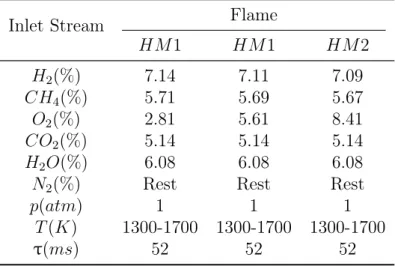
Table 2.2: PSR operating conditions (compositions are as mass fractions of the total inlet stream)

Inlet Stream Flame

HM 1 HM 1 HM 2 H2(%) 7.14 7.11 7.09 CH4(%) 5.71 5.69 5.67 O2(%) 2.81 5.61 8.41 CO2(%) 5.14 5.14 5.14 H2O(%) 6.08 6.08 6.08

N2(%) Rest Rest Rest

p(atm) 1 1 1

T (K) 1300-1700 1300-1700 1300-1700

⌧(ms) 52 52 52

The results are very similar for each Flame (HM1, HM2, HM3) and for any temperature chosen in the range 1300 - 1700 K, so no modifications in the simplified mechanism will be taken into account. Instead, some differences may be noticed using Glarborg [19] and POLIMI [42] detailed kinetic schemes, in terms of main reactions involved in NO and intermediate species formation, how it is possible to see in Figure 2.2 and in Appendix B. Thus, two different simplified mechanism will be considered. Rate of production analysis (Figure 2.2) shows that under jet flames in a diluted hot coflow conditions, so temperature below 1700 K and locally

1_{k = AT exp( E} a/RT )

Rate of Production Analysis - NO 242 HO2+NO=NO2+OH -0.027 342 CH3+NO2=CH3O+NO 0.020 298 NH+NO=N2O+H 0.016 243 NO2+H=NO+OH 7.02e-03 299 NH+NO=N2O+H -4.21e-03 253 HNO+H=H2+NO 2.03e-03 338 HCO+NO=HNO+CO -1.38e-03 347 C2H3+NO=C2H2+HNO -1.21e-03 319 NNH+O=NH+NO 1.13e-03 238 H+NO+M=HNO+M 1.01e-03 306 N+NO=N2+O 8.57e-04 305 N+O2=NO+O 7.17e-04 297 NH+O2=NO+OH 6.90e-04 239 H+NO+N2=HNO+N2 3.62e-04 336 CO2+N=NO+CO 1.65e-04 241 OH+NO+M=HONO+M 9.07e-05 334 CO+NO2=CO2+NO 7.52e-05 329 N2O+O=2NO 6.46e-05 256 HNO+O2=HO2+NO 4.97e-05 255 HNO+OH=NO+H2O 4.12e-05 (a)

Rate of Production Analysis - NO

622 NO+HO2=NO2+OH -0.040 694 CH3+NO2=CH3O+NO 0.026 657 NO2+H=NO+OH 0.012 690 NH+NO=N2O+H 0.012 627 HNO+H=NO+H2 3.04e-03 686 C2H3+NO=C2H2+HNO -1.88e-03 624 NO+OH+M=HONO+M 1.87e-03 603 NNH+O=NH+NO 1.65e-03 625 HCO+NO=CO+HNO -1.34e-03 626 H+NO+M=HNO+M 1.16e-03 573 NH+O2=NO+OH 8.75e-04 580 N+NO=O+N2 7.75e-04 579 N+O2=NO+O 7.12e-04 696 NO+CH4=HNO+CH3 1.61e-04 681 CO2+N=NO+CO 1.36e-04 691 N2O+O=2NO 1.16e-04 630 HNO+O2=NO+HO2 9.15e-05 664 CO+NO2=CO2+NO 7.67e-05 629 HNO+OH=NO+H2O 6.51e-05 684 CH2+NO=NCO+H2 -6.02e-05 (b)

Figure 2.2: NO Rate of production analysis (ROPA) for Glarborg (a) and POLIMI (b) mechanism. Blue lines indicate NO destruction, while the red ones NO formation.

fuel-rich flame, NO formation may occur via different routes. In fact, it is possible to notice that HNO and NO2 are significant educts for NO formation and, unlike

Löffler et al. mechanism [18], not completely converted back. Thus, they become important in this condition, like NNH/NH and N2O route, while thermal NO route

is not so relevant at these temperature.

It is also possible to apply ROPA approach to evaluate the main reactions in-volving the intermediate species N, N2O, NO2, NNH, NH, HNO, HONO, NH2,

NH3, which are listed in Appendix B both for Glarborg [19] and POLIMI [42]

kinetic mechanism. Considering that the reactions forming NO from the interme-diate species are relative slow, it is possible to apply the same hypothesis made by Löffler et al. [18] (Section 1.2.1). Therefore, the concentration of these species can be obtained by a set of nine algebraic equation linear in terms of the unknowns, which can be solved analytically. In order to calculate the reverse rate constants, OpenSMOKE [41] has been applied again.

[N ] = kr1[O][N2] + kr2[N O][O] + kr22[N O][CO] + kf 17[N H][H]

kf 1[N O] + kr2[O2] + kf 22[CO2] + kr4[H2] (2.1)

[N2O] =

kr4[O][N2][M ] + kr18[N2][OH] + kr23[N2][CO2] + kf 15[N H][N O]

kf 4[M ] + kf 18[H] + kf 23[CO] + kr15[H] (2.2)

[N H] =kr26[N O][OH] + [N H2](kf 27[OH] + kf 24[H]) + kr15[N2O][H] + kf 8[N N H][O] + kr25[HN O][O] [O2](kf 25+ kf 26) + kr27[H2O] + kr24[H2] + [N O](kf 15+ kr8 (2.3)

[HN O] = [N O](kr28[H2] + kf 29[CH4] + kr30[HO2] + kf 31[H][M ] + kf 32[HCO]) + kf 25[N H][O2]

kf 28[H] + kr29[CH3] + kf 30[O2] + kr31[M ] + kr32[CO] + kr25[O] (2.4)

[N O2] =

[N O](kf 33[HO2] + kr34[CH3O] + kr35[OH]) + kr36[HON O][H]

kr33[OH] + kf 34[CH3] + kf 35[H] + kf 36[H2] (2.5)

[HON O] =[N O2](kr36[H2] + kr38[CH4] + kf 39[HO2]) + kf 37[N O][OH][M ]

kf 36[H] + kf 38[CH3] + kr39[O2] + kr37[M ] (2.6) [N H2] = [N H3](kr40[H] + kf 41[OH] + kr42[CH3]) + kr24[N H][H2] kf 40[H2] + kr41[H2O] + kf 42[CH4] + kf 24[H] (2.7) [N H3] =[N H2](kf 40[H2] + kr41[H2O] + kf 42[CH4]) kr40[H] + kf 41[OH] + kr42[CH3] (2.8) [N N H] =[N2](kr21[HO2] + kr7[H] + kr20[H][O2]) kf 21[O2] + kf 7+ kf 20[O2] (2.9)

[CH3O] =

[CH3](kf 44[HO2] + kf 45[O2]) + kr43[CH2O][H][M ]

kr44[OH] + kr45[O] + kf 43[M ] (2.10)

In order not to overload the present Chapter, only the expressions deduced via POLIMI [42] mechanism have been reported. For further details see Appendix B. Moreover, an additional algebraic equation for CH3O has been added since

this specie is not available in all kinetic scheme used in combustion calculations. Instead, the concentrations of O2, N2, H2, H2O, O, H, OH, HO2, CH3, CH4, CO,

CO2, HCO, CH2O can be known from combustion calculations.

Finally, the rate of NO formation is given by: d[N O] dt = ⇣ kr33[N O2][OH] + kf 34[N O2][CH3] + kf 35[N O2][H] ⌘ + + kr15[N2O][H] + ⇣

kf 28[HN O][H] + kr37[HON O][M ]+

+ kr32[CO][HN O] + kr31[HN O][M ] ⌘ +⇣kf 8[N N H][O] + kf 26[N H][O2] ⌘ +⇣kr1[O][N2] + kf 2[N ][O2] ⌘ . (2.11)

2.3 Numerical modeling

The numerical modeling is based on a previous work by Aminiam et al. [40], characterized by a good prediction with experimental data. The main point still remains the validations of the new models.

2.3.1 Computational domain and grid

The geometry of the burner allows to use a 2D axisymmetric domain (Figure 2.1b), constructed from the burner exit. A computational grid with 73x340 (24 k) cells has been constructed (Figure 2.3). The thicknesses of the walls between the central fuel jet and the coflow and between the coflow and the tunnel air have been neglected. In fact, these thicknesses are of 0.2 and 2.8 mm, respectively.

2.3.2 Boundary Conditions

In order to improve the convergence and simulation time, a zero-shear stress wall was adopted at the side boundary, instead of a more realistic pressure inlet/outlet conditions, in according to Aminiam et al. [40]. However, as the tunnel air was considered wide enough, this boundary condition did not affect the flame structure.

Figure 2.3: Computational domain, mesh grid and boundary conditions [40]

Uniform velocity and composition profiles, presented in Table 2.1, are given to the unmixed fuel jet and coflow oxidizer. The tunnel air inlet stream is provided at room temperature at the same velocity as the hot coflow. In according with precedent studies [40], great importance has been dedicated to the inlet turbulence level of all inlet streams, in order to better describe the development of the mixing layers. In particular, the turbulent kinetic energy (TKE) of the fuel and coflow inlet were set to 60 m2_/s2 _{and 0.43 m}2_/s2 _{as suggested by Christo and Dally [37]}

and Frassoldati et al. [38], respectively. To enhance the mixing in the shear layer between coflow and tunnel air streams, the tunnel air inlet TKE was set to 0.15 m2_/s2_{, in according to Aminiam et al. [39]. The experimental data profile [35] of}

NO mass fraction, measured at axial coordinate z = 4 mm, was set as boundary condition for coflow. Subsequently, others simulations were carried out imposing the experimental data profile for temperature and main species of fuel jet and coflow, instead of the fixed values reported in Table 2.1.

2.3.3 Physical Model

A brief description of the physical model used is provided in this section. For further details about the main topics consult Section 3.2.

The steady-state Favre-Averaged Navier-Stokes (FANS) equations were solved with a finite volume scheme using the commercial CFD code FLUENT®_{. The}

turbulence model employed is the k-✏ model using all standard constants, except for C✏1, which is set to 1.6 instead of 1.44, in according to Aminiam et al. [40].

The full KEE mechanism (17 species and 58 reversible reactions) of Bilger et al. [43] was used. The interaction between turbulence and chemistry was handled by the EDC model [44] with the employment of the in-situ adaptive tabulation (ISAT) method of Pope [45] with various error tolerances, in order to reduce computational

time. The fine structure residence time constant in the EDC model, which equals to C⌧ = 0.4083, was set to higher values of 1.5 in order to enhance the prediction

of experimental data, in according to Aminiam et al. [40].

The discrete ordinate (DO) method together with the Weighted-Sum- of-Gray-Gases (WSGG) model with coefficients taken from Smith et al. [46] was employed to solve the radiative transfer equation (RTE) in 16 different directions across the computational domain.

As far as NO formation is concerned, two additional formation routes have been considered, beside the conventional thermal and prompt ones. In particular, the N2O intermediate and NNH routes have been also included in the modeling

ap-proach, to account for low-temperature formation mechanisms and for the presence of H2 in the fuel. The NNH route is not directly available in the code; therefore, it

has been implemented by means of a user-defined function (UDF) following Kon-nov et al. [17]. For thermal and NNH intermediate mechanisms, the radical mass concentrations, i.e. O, H, OH, are supplied by the detailed kinetic mechanism with-out any equilibrium or partial equilibrium hypothesis (Chapter 1). Beside these models, the Löffler et al. mechanism [18] and the simplified models described in Section 2.2 have been implemented also by means of UDF. For all the routes, a probability density function (PDF) for temperature to take turbulence effects into account was considered.

A summary of the carried out numerical simulations is listed in Table 2.3.

2.4 Results

This Section will be focused on the comparison between the different approaches adopted for the prediction of NO emissions from the JHC burner. A proper pre-diction of the NO trends is mandatory, being flameless combustion an appealing technology for reducing NOx pollutants. MILD combustion typically occurs at

lower temperatures so that other mechanisms, such as the N2O, NO2 and HNO

route, may become dominant. Moreover, when hydrogen is added to the fuel, the NNH path may play a significant role.

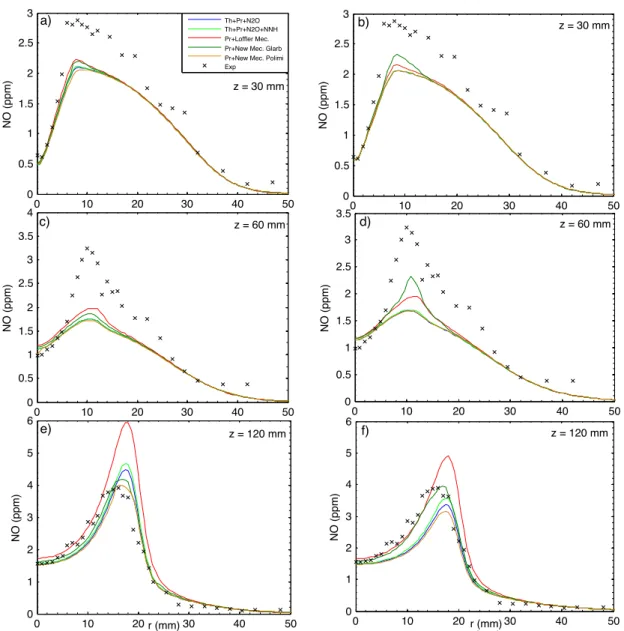
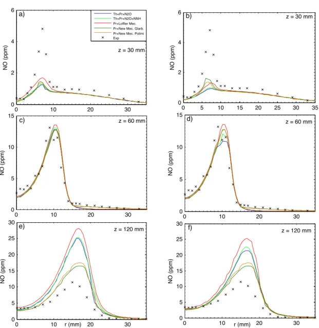
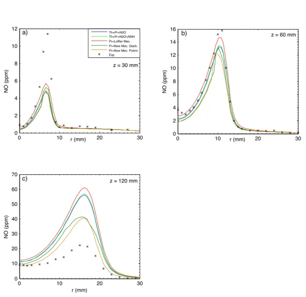
In this section the two new mechanisms derived from Glarborg [19] and POLIMI [42] detailed kinetics schemes have been compared with others NO formation mech-anisms, such as Löffler et al. [18]. The numerical values of NO concentration (ppm), at the exit of combustion chamber and for all the models investigated, are listed in Table 2.4. Predicted and measured radial profiles of NO concentration at three axial locations for each flame are illustrated in Figures 2.4 2.5 2.6. Particular

at-Table 2.3: Details of the numerical simulations for NO evaluation in JHC burner

N. Flame Species B.C. NO Model

1 HM1 Constant Pr+Th+N2O

2 HM1 Constant Pr+Th+N2O+NNH

3 HM1 Constant Pr+Löffler Mec.

4 HM1 Constant Pr+New Mec. Glarb. 5 HM1 Constant Pr+New Mec. POLIMI.

6 HM2 Constant Pr+Th+N2O

7 HM2 Constant Pr+Th+N2O+NNH

8 HM2 Constant Pr+Löffler Mec.

9 HM2 Constant Pr+New Mec. Glarb. 10 HM2 Constant Pr+New Mec. POLIMI.

11 HM3 Constant Pr+Th+N2O

12 HM3 Constant Pr+Th+N2O+NNH

13 HM3 Constant Pr+Löffler Mec. 14 HM3 Constant Pr+New Mec. Glarb. 15 HM3 Constant Pr+New Mec. POLIMI.

16 HM1 Profile Pr+Th+N2O

17 HM1 Profile Pr+Th+N2O+NNH

18 HM1 Profile Pr+Löffler Mec.

19 HM1 Profile Pr+New Mec. Glarb. 20 HM1 Profile Pr+New Mec. POLIMI.

21 HM2 Profile Pr+Th+N2O

22 HM2 Profile Pr+Th+N2O+NNH

23 HM2 Profile Pr+Löffler Mec.

24 HM2 Profile Pr+New Mec. Glarb. 25 HM2 Profile Pr+New Mec. POLIMI.

Table 2.4: Predicted NO emissions with different models for different flame Flame Th+Pr+N2O Th+Pr+N2O+NNH Pr+Loffler Mec. Pr+New Mec.

HM1 7.7 8.7 13.3 13.3

HM2 15.1 16.8 17.3 19.8

tention has been paid to evaluate the level of agreement between the new simplified models and experimental data. In each figure is also shown the comparison between the case with constant value and experimental profile boundary conditions.

Observing the following figures, it is worth noting that at the upstream (z = 30 mm) all the models used under-predict NO concentration. This is particularly true for HM2 and HM3 flame. Little better results have been achieved imposing the radial profile of the main species and temperature as boundary conditions for coflow, instead of constant values. At z = 60 mm the new simplified models and Löffler et al. [18] mechanism are in good agreement with experimental data, except for HM1 flame. It is worth noting also that at the downstream (z = 120 mm) the new simplified models capture better the general trend respect to the others models, with an overestimation of 2% for HM1, 15% for HM2 and 35% for HM3. On the whole, it is possible to summary that experimental data are accurately predicted by the New Models, especially considering the order of magnitude (ppm).

The relative importance of the different NO formation routes is shown in Figures 2.7-2.9. It can be observed that the thermal route is almost negligible in all cases, due to the low temperatures, typical of MILD combustion. In particular, the higher the oxygen level in coflow (HM2 and HM3), the less important the above-mentioned route becomes. Prompt pathway is the major source of NO (about 50% of the total) because of the local fuel-rich conditions. Beside it, N2O and NNH

routes play an important role in the overall NO formation. The former has great percentage importance in HM1 (about 20% in Löffler mechanism), but decreases at the increment of oxygen (9% in HM2 and 5% in HM3). The NNH route is expected since the availability of H radicals in the flame and it has a direct impact on the formation of NO. In particular, the NNH contribution appears to be stable at around 20% in each flame and in both Löffler mechanism and the New Model. Considering the New Model, it can be observed the relative importance of HNO and NO2 route (11% in HM1, 10% in HM2 and 7% in HM3), which cannot be

0 10 20 30 40 50 0 0.5 1 1.5 2 2.5 3 NO (ppm) z = 30 mm 0 10 20 30 40 50 0 0.5 1 1.5 2 2.5 3 NO (ppm) z = 30 mm 0 10 20 30 40 50 0 0.5 1 1.5 2 2.5 3 3.5 4 NO (ppm) z = 60 mm 0 10 20 30 40 50 0 0.5 1 1.5 2 2.5 3 3.5 NO (ppm) z = 60 mm 0 10 20 30 40 50 0 1 2 3 4 5 6 r (mm) NO (ppm) z = 120 mm 0 10 20 30 40 50 0 1 2 3 4 5 6 r (mm) NO (ppm) z = 120 mm Th+Pr+N2O Th+Pr+N2O+NNH Pr+Loffler Mec. Pr+New Mec. Glarb Pr+New Mec. Polimi Exp c) e) b) d) f) a) r (mm) r (mm)

Figure 2.4: Comparison between measured and predicted radial profiles of NO, in constant (a-c-e) and experimental profile (b-d-f) boundary conditions for flame HM1.

0 10 20 30 0 2 4 6 NO (ppm) z = 30 mm 0 5 10 15 20 25 30 35 0 2 4 6 NO (ppm) z = 30 mm 0 10 20 30 0 5 10 15 NO (ppm) z = 60 mm 0 10 20 30 0 5 10 15 NO (ppm) z = 60 mm 0 10 20 30 0 5 10 15 20 25 30 r (mm) NO (ppm) z = 120 mm 0 10 20 30 0 5 10 15 20 25 30 r (mm) NO (ppm) z = 120 mm Th+Pr+N2O Th+Pr+N2O+NNH Pr+Loffler Mec. Pr+New Mec. Glarb. Pr+New Mec. Polimi Exp a) c) e) d) b) f)

Figure 2.5: Comparison between measured and predicted radial profiles of NO, in constant (a-c-e) and experimental profile (b-d-f) boundary conditions for flame HM2.

0 10 20 30 0 2 4 6 8 10 12 r (mm) NO (ppm) z = 30 mm 0 10 20 30 0 2 4 6 8 10 12 14 16 r (mm) NO (ppm) z = 60 mm 0 10 20 30 0 10 20 30 40 50 60 70 r (mm) NO (ppm) z = 120 mm Th+Pr+N2O Th+Pr+N2O+NNH Pr+Loffler Mec. Pr+New Mec. Glarb. Pr+New Mec. Polimi Exp

a)

c)

b)

Figure 2.6: Comparison between measured and predicted radial profiles of NO for flame HM3.

0%# 10%# 20%# 30%# 40%# 50%# 60%# 70%# 80%# 90%# 100%# Th+P r+N2O # Th+P r+N2O +NNH# Pr+Loffl er#Me c.# Pr+N ew#Me c.#Glar b.# N O #(%# pp m )# HNO+NO2# NNH# N2O# Pr# Th#

Figure 2.7: Relative importance of NO formation routes for flame HM1

0%# 10%# 20%# 30%# 40%# 50%# 60%# 70%# 80%# 90%# 100%# Th+P r+N2O # Th+P r+N2O +NNH# Pr+Loffl er#Me c.# Pr+#N ew#Me c.# N O #(%# pp m )# HNO+NO2# NNH# N2O# Pr# Th#

Figure 2.8: Relative importance of NO formation routes for flame HM2.

0%# 10%# 20%# 30%# 40%# 50%# 60%# 70%# 80%# 90%# 100%# Th+P r+N2O # Th+P r+N2O +NNH# Pr+L offler# Mec.# Pr+N ew#Me c.# N O #(%# pp m )# HNO+NO2# NNH# N2O# Pr# Th#