Chapter 2 Vehicle Model

Chapter 2

Vehicle Model

2.1

Vehicle Model

To examine car behavior a vehicle model was built using the software “Simulink”. In this chapter the theoretical aspects are described, but in the next one we focus more specifically on the model actually built.

The model is a four wheeled model, in fact to consider only a simpler and surely more common “Single Track Model” ( [6], [11]) is not possible on account of several reasons

• Some simplifications used to justify the “Single Track Model” are not valid if only one wheel is braked1_{, as occurs when the ESP is acting.}

• To find a strategy to control the distribution of torque and to model the ESP it is necessary to analyze individual wheel speeds.

• We were interested in studying vehicle behavior in critical conditions (for example a car that is spinning around).

The vehicle is modeled as a rigid body in 2-D; car motions are possible in the horizontal x − y plane, the wheels have no mass but an inertia moment different from zero. The steer axes are considered exactly vertical and passing through the wheel symmetry planes and the wheel spin axes.

The street is schematized like perfectly flat (no slope and roughness). the model is characterized by 7 d.o.f.

More details are shown subsequently.

1

Indeed in the “Single Track Model” the left and the right tyre of an axle must transfer the same longitudinal force

2.1.1

Vehicle equations

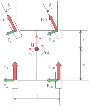
Considering the simplifications mentioned above it is possible to build a model based on the subsequent system of equations [6] (see also fig. 2.1):

Figure 2.1: Representation of the principal model quantities

m( ˙u − vr) = X = (Fx11+ Fx12) cos δ − (Fy11+ Fy12) sin δ + (Fx21+ Fx22) −

1 2rCxu

2 _(2.1)

m( ˙v + ur) = Y = (Fx11+ Fx12) sin δ + (Fy11+ Fy12) cos δ + (Fy21+ Fy22) + FL (2.2)

J˙r = N = ((Fx11+ Fx12) sin δ + (Fy11+ Fy12) cos δ)a − (Fy21+ Fy22)b+

−((Fx11− Fx12) cos δ + (Fx21− Fx22) − (Fy11− Fy12) sin δ)t₂ + FLe

(2.3)

Jw,nm˙ωnm = Mnm− Fx,nmHnm− Mb,nm, n, m= 1, 2. (2.4)

Although the equations are quite general and not linearized, they present some simpli-fications, for example

• The drag force is applied along the car symmetry axis, without considering lateral actions.

• The external force FL is a pure side force (it does not have drag component).

• The vertical deformations of the tyres are ignored.

• The center of gravity is placed on the car symmetry axis.

2.1.2

Vertical Load

To describe correctly the tyre behavior, knowing the vertical load acting on each wheel, is essential for our problem. In our model only the effect of lateral load transfer is modelled, ignoring modest effects of longitudinal load transfer. We used the following relations, in which we consider the vehicle in a steady state, not to make the problem uselessly compli-cated.

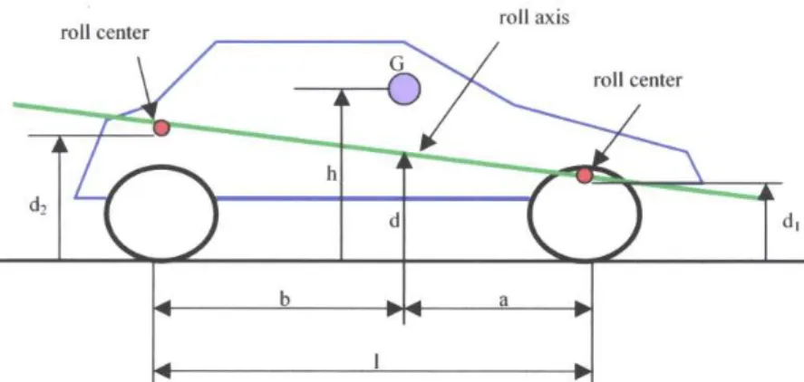
Figure 2.2: Lateral view of the vehicle scheme For the lateral balance of the whole vehicle

Fy1+ Fy2+ FL = Y = mur (2.5)

Fy(1,2) are the global side forces respectively of the front and the rear axle.

For the rotational balance of suspended mass with respect to the roll axis (supposed horizontal and at a distance d = bd1+ad2

l from the ground)

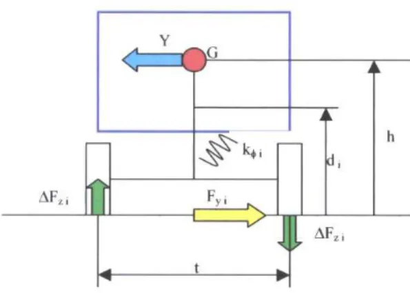
Figure 2.3: Frontal view of the vehicle scheme

The lateral force (FL), that for example can be considered a representation of lateral

wind, is applied at the same height of the center of gravity. Also this assumption is a simplification.

For rotational balance of each axle (considered with mass equal to zero), with respect to the rolling axis

−∆Fziti+ Fyidi+ kφiφ = 0 (2.7)

Using the previous system of equations, calling Y −FL= ¯Y, we can obtain the following

results ∆Fz1 = (Fy1d1+ kφ1 ¯ Y(h − d) kφ )1 t (2.8) ∆Fz2 = (Fy2d2+ kφ2 ¯ Y(h − d) kφ )1 t (2.9)

Where kφ1,2 are the front and rear axle rolling stiffnesses, kφ is the sum of the two

stiffnesses, d1,2 are the heights of the front and the rear axle roll centers, d is the roll axis

height under the mass center, and in the end h is the mass center height, as shown in fig.2.2 and fig.2.3.

2.1.3

On Demand Drive

Our model represents an on demand drive car. In this kind of vehicles the engine torque is normally directed towards the front or the rear axle but by means of some devices we can split it, such a way to provide torque to all the wheels. It can be really useful in

some situations, for example if the driver is speeding up so hard to make the tyres slip. In fact during a transitory like that we waste uselessly part of the engine power then we do not obtain the maximum possible acceleration and in the same time we can have an excessive wear and tear of the tyres. Sharing the drive torque between the two axles we can avoid these phenomena and improve the vehicle performances. Moreover also the car handling is affected by the drive torque flow. These considerations make us understand that we would like to choose the torque distribution just depending on the configuration which allows the best vehicle performances. Unfortunately this is not possible, at least using conventional apparatuses. Indeed to realize an on demand drive we must equip the vehicle with a central coupling (for example it can be a clutch or a viscous coupling) and they are able just to transfer a part of the whole drive torque. For example, considering a rear-wheel drive vehicle (which torque distribution is 0% − 100%), we can imagine to be allowed to reach a situation in which we have 50% − 50%, but in normal friction conditions we cannot obtain a total inversion of the torque, that is to say 100% − 0%.

We modelled a car provided with an “Haldex” coupling, which is similar to a central clutch, but it can be controlled to regulate the torque flow.

Haldex Coupling

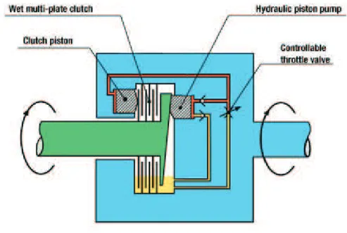
The “Haldex” central coupling is schematically represented in fig.2.4. There is a housing,

connected with the right shaft, which is in turn connected with one of the two differentials installed on the car. This housing has inside the external discs of a wet multi-plate clutch through which torque can be transmitted from the front axle to the rear (or vice versa), a little hydraulic circuit, a valve to control the liquid pressure, a little hydraulic piston pump and a clutch piston that can press the clutch plates each other. The left shaft (linked with the other differential) is connected with the internal clutch plates. At its end, inside the housing, a cam that activates the pump is realized. The pump will only be active when the front and the rear axles rotate at a different speed. The liquid pressure pushes the clutch piston, which engages the clutch. In this way a certain amount of torque is transmitted from the shaft which receives directly the engine torque to the other one. By means of the valve, controlled by a CPU receiving information from several sensors installed on the vehicle (steering wheel position, wheel speeds, lateral acceleration, etc.), it is possible to control the pressure inside the hydraulic circuit, such a way to arrange the amount of transferred torque. For example this valve nullifies the pressure if the car is moving very slow, not to compromise the handling, or while some electronic devices (for example the ABS) are acting. The valve is also a safety system as it limits pressure in case the amount of transmitted torque is too high and it can damage the coupling.

Coupling Model

To model the “Haldex” coupling the subsequent equations are used (see also fig.2.5)

ωr = ω21_2τ+ωd22

ωf = ω11_2τ+ω_d12

(2.10)

τd is the differential transmission ratio, ωf,r are respectively the front and the rear drive

shaft rotational speeds.

ωr − ωf is the input to calculate Tf0 by a function like that represented in fig. 2.62.

Tf0 is the transmitted torque in case the valve is completely closed. To simulate the valve

Figure 2.6: “Haldex” coupling characteristic

chocking Tf0 is multiplied by a coefficient included between 0 and 1.

In our model we did not take into account the fact that when the shaft speeds are such a way to produce a transferred torque, this effect cannot be instantaneous. For example one of the causes of this delay is the fact that the liquid pressure must increase to engage the clutch, then to transfer torque, and this phenomenon takes some time. However, as reported in ( [7], [5]), this delay is so short that it can be ignored. Moreover it is possible to notice that the shaft inertiae were neglected, but the system dynamics is influenced by the wheel inertiae.

2

The description of the Haldex coupling refers to a rear-wheel drive car, but to model a front-wheel drive car is sufficient to exchange ωrfor ωf in (2.10).

2.2

Tyre Model

Capturing the tyre behavior is probably the most difficult and important problem to tackle while building a vehicle model as realistic as possible. In the past a lot of different models have been created to try to solve this problem. The most realistic models are the most complicated but probably they are not useful in every kind of research. On account of our objectives a too simple model (for example the linear model suggested in [6]) is not applicable because it can provide correct results only if the slip angles are very small, but it cannot represent for example the forces that tyres transfer during a spin manoeuvre. For these reasons we chose the Semi-Empirical model suggested in [10], which proved to be a good model but not too complicated.

2.2.1

Reference Frame

To define the reference frame and some others quantities is useful to understand the fol-lowing description of the model.

As shown in figure 2.7 we consider a levorotatory set of three perpendicular axes in which the x axis is the intersection of the wheel symmetry plane with the ground (the positive direction is the wheel center longitudinal speed direction), the y axis is the projec-tion of the wheel spin axis on the ground, and the z axis as a consequence (with upwards positive direction).

2.2.2

Slip Quantities

Longitudinal Slip

The longitudinal slip (k) is defined as

k = −Vx− reω

Vx = −

ω0− ω ω0

, (2.11)

Where re is the effective rolling radius in free rolling conditions, ω is the instantaneous

wheel rotational speed and ω0 is the wheel rotational speed in free rolling condition at the

given Vx.

Slip Angles Equations and Lateral Slip

We define the slip angle (α) as the angle formed between the wheel x axis and the wheel center speed vector. It is positive if we need to rotate the x axis in clockwise turn (see fig.2.8) to put it over the speed vector. Also interesting is to realize that in our reference frame a positive slip angle matches with a positive lateral force. To calculate the slip angles the following equations reported in [6] are used. We want to remark the fact that these equations are obtained just by simple kinematic relations and they are independent from any specific tyre model. Nevertheless they are useful only if connected with a tyre scheme.

Figure 2.8: Definition of slip angle (top view)

tan (δ − α11) = v+ ra u − rt₂ (2.12) tan (δ − α12) = v+ ra u+ rt 2 (2.13)

tan (−α21) = v − rb u − r₂t (2.14) tan (−α22) = v − rb u+ rt 2 (2.15) Also these equations have been used without applying the simplifications usually con-sidered since we want to build a model which can represent vehicle dynamics even during critical manoeuvre.

The lateral slip is defined as “ tan α”.

We want to point out the fact that all the relations exposed in this paragraph are valid considering for each wheel a reference frame in which the x axis has every instant the same positive direction as the longitudinal wheel center speed vector. To take this fact into account the real model presents some differences with respect to theoretical relations. Theoretical slip quantities

It will prove to be useful also to define the theoretical slip quantities σx = k 1 + k (2.16) σy = tan α 1 + k (2.17) σ∗ ₌q_σ2 x+ σ2y (2.18)

2.2.3

Semi-Empirical Model

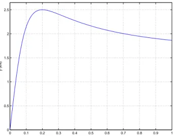
The most famous and general expression for this model is the following function, usually called “Magic Formula” ( [6], [10], [11])

y(x) = D sin (C arctan (Bx − E(Bx − arctan (Bx)))) (2.19) Where y(x) is Fx or Fy respectively if x is k or α. A typical curve shape obtained by the

Magic Formula is shown in figure 2.9.

The parameters which appear in the Magic Formula are respectively B : stiffness factor

C : shape factor D : peak factor

0 0.1 0.2 0.3 0.4 0.5 0.6 0.7 0.8 0.9 1 0 0.5 1 1.5 2 2.5 x y (kN)

Figure 2.9: Curve obtained by Magic Formula (D = 2.5kN, C = 1.6, BCD = 30kN, E = 0) E : curvature factor

These factors can be constant values or they can be in turn functions of some others variables (vertical load, camber angle, etc.).

We considered only the influence of vertical load on wheel forces, using the following relations ( [6], [10])3_: Dy = µyFz = (a1Fz+ a2)Fz (2.20) BCDy = a3sin (2 arctan ( Fz a4 )) (2.21) Ey = (a6Fz+ a7) (2.22) Dx = µxFz = (b1Fz+ b2)Fz (2.23) BCDx = (b3Fz2+ b4Fz) exp (−b5Fz) (2.24) Ex = (b6Fz2+ b7Fz+ b8) (2.25)

(a1,2,3,4,6,7 and b1,2,3,4,5,6,7,8 are suitable constant values.)

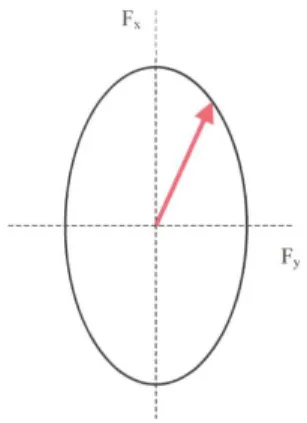
Values obtained by (2.19) however are not correct to represent the tyre behavior in com-bined slip conditions. The fact that longitudinal and lateral forces influence each other is well-known, and for this reason to improve the tyre model such a way to build an ellipse of grip is necessary (fig.2.10).

3

Figure 2.10: Ellipse of grip

A possible way to modify the model is suggested in [11]. This method is very practical because it needs just the force functions the tyre produces in pure slip conditions (they are represented by means of a function as (2.19)). In fact, starting from the global theoretical slip (σ∗_{) we calculate, by means of the inverse formulae, the slip quantities k and α which}

would produce σ∗ _{in pure slip conditions. Then, considering this two values as inputs in}

the pure slip force functions we calculate Fx0 and Fy0. In the end we estimate Fx and Fy

through the following equations (in (2.26) and (2.27) σxand σy are the actual instantaneous

theoretical slips). Fx = σx σ∗Fx0(σ ∗_{) (2.26)} Fy = σy σ∗Fy0(σ ∗_{) (2.27)}

To represent better tyre behavior during transitories to insert a first order filter was considered useful, as suggested in [6]:

L Vx

d ˜f

dt + ˜f = f (2.28)

L is the tyre relaxation length and f can be k or tan α.

Actually the input to calculate F(x,y)0 is ˜σ∗(t), obtained using in (2.18) ˜k(t) and ]tan α(t).

We want to stress that ˜k(t) and ]tan α(t) are functions depending on the time. In this manner the tyre performance does not present any discontinuities. This kind of response is more realistic whereas a tyre needs to be deformed to transfer forces and this phenomenon cannot be instantaneous, hence tyre forces do not present any discontinuities.