1 Description of Scattering Problems

CHAPTER

1

Description of Scattering Problems

Abstract- This chapter summarizes a number of concepts from

electromagnetic field theory used in numerical formulation for scattering problems. Integral and differential equations for the surface current induced on a conducting scatterer are derived using boundary conditions on the electric and magnetic fields. Expressions are developed for calculating the scattering cross section of an object.

1.1 MAXWELL’S EQUATIONS

In many practical systems involving electromagnetic waves, the time variations are of sinusoidal form and are referred to as time harmonic [1]. In general, such time variations are represented by j t

eω and the instantaneous electromagnetic field vectors are related to their complex forms. In a linear and isotropic medium, any solution for the time-harmonic electric and magnetic fields must satisfy Maxwell’s equations

0 0 0 0 0 0 , , ( ) , ( ) , r r ev r r em r r E M j H H J j E q E q H

ωμ μ

ωε ε

ε ε

ε ε

μ μ

μ μ

∇× = − − ∇× = − ∇ ⋅ = ∇ ⋅ = ur uur uur uur ur ur ur uur (1.1)

where Eur and uurH are the electric and magnetic fields respectively, and the time dependence ej tω is implicit. The behaviours of both the electric and magnetic fields are described by Maxwell’s equations, which, for the purpose of this work, are expressed in a frequency domain. In regions where there are no sources, J =M =qev =qem =0

ur uur

,

the previous equations are of simpler form. Whereas the electric current density Jur may

represent either actual or equivalent sources, the magnetic current density Muur can only

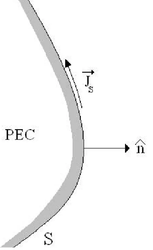
represent an equivalent source. The study of typically electromagnetic problems involves the application of equations (1.1) to a specific geometry and their subsequent solution to determine the fields, the fields scattered in some direction by the presence of some objects, or some similar observable quantity. In this context, boundary conditions are very important in order to determine a unique solution of the electromagnetic problem. Regions containing penetrable dielectric or magnetic material may be bounded by material having a very high conductivity, which is often approximated by infinite conductivity and termed a perfect electric conductor (PEC). In the limit of infinite conductivity we denote the surface of a perfect electric conductor as a boundary of the problem domain. On such a boundary, the electric and magnetic fields vectors satisfy the conditions

$ $ $ $ 0 0, , , 0, s s r n E n H J n E n H

ρ

ε ε

× = × = ⋅ = ⋅ = ur uur uur ur uur (1.2)

where $n is the normal vector to the surface that points into the problem domain, Js

ur is

Fig. 1.1 Current on a PEC

Maxwell’s equations are used to develop integral equations, which are often chosen as the starting point for electromagnetic scattering problems. A typical scattering problem is to determine the scattered fields when a material obstacle, represented by relative

permittivity

ε

_r and permeability

μ

_r, is introduced in a free space region where fields

,

inc inc

E H

ur uur

were previously generated by some sources located somewhere. This problem is characterized by a heterogeneous environment and is well described by equations (1.1) with the necessary modifications. In order to simplify the formulation of integral equations, it is convenient to convert the original scattering problem into an equivalent problem by applying the volumetric equivalence principle. We can replace the dielectric body or magnetic material present in the original problem by equivalent induced polarization currents and charges. In this way, Maxwell’s equations can be rewritten to produce

0 0 , , ( ) , ( ) , o e o m E j H M H j E J E H

ωμ

ωε

ε

ρ

μ

ρ

∇× = − − ∇× = − ∇ ⋅ = ∇ ⋅ = ur uur uur uur ur ur ur uur (1.3) where 0 0 ( 1) , ( 1) , r r M j H J j E

ωμ μ

ωε ε

= − = − uur uur ur ur (1.4)

are the equivalent magnetic and electrical current densities, respectively. Equations 1.3 describe the same fields as equations (1.1), but involve a homogeneous space

characterized by permittivity

ε

o and permeability

μ

o instead of the original

heterogeneous environment. The new equivalent sources of (1.4) radiate in free space. The task of finding electromagnetic fields in free space is much more straightforward than the original burden of solving equations (1.1) directly in the inhomogeneous environment. The volume equivalent current densities are most useful for finding the fields scattered by dielectric obstacles. The fields scattered by perfectly conducting surfaces can best be determined by using surface equivalent densities.

1.2 DESCRIPTION OF SCATTERING PROBLEM

In this section, a general description of a scattering problem [1] [2] is made in order to obtain a relationship between the induced currents and the electric and magnetic fields. Wave propagation is examined in the presence of objects of various geometries. This is accomplished by introducing an additional component to the total field, referred as the scattered field, due to the presence of the targets.

Suppose the scatterer of Fig. 1.2 is illuminated by a field produced by a source, called primary source, located somewhere outside the scatterer.

PEC

Region 2

Region 1

ε μ

1 1

source

J

E, H

J

n

Fig. 1.2 Scattering problem involving a PEC body

The total fields can be divided into two parts

, , inc scat inc scat E E E H H H = + = + ur ur ur

uur uur uur (1.5)

where Huurinc and Eurincare the fields produced by the primary source in absence of any

scatterer, Huurscat and Eurscat are the fields due to the scatterer, which also radiate in free space. The incident fields in the immediate vicinity of the scatterer, away from its source, satisfy the vector Helmholtz equations

and the scattered fields are solutions to the equations

2 2 0 0 2 2 0 0 , , scat scat scat scat J E k E j J M j J H k H J j M j

ωμ

ωε

ωε

ωμ

∇∇ ⋅ ∇ + = − + ∇× ∇∇ ⋅ ∇ + = −∇× + − ur ur ur ur uur ur

uur uur ur uur (1.6)

where Jur and Muur denote the equivalent sources defined by the volumetric equivalent

There are different approaches to finding the solution of equations 1.6 and 1.7 in homogeneous and infinite space. As shown in fig. 1.3 path a, one approach to obtaining the fields is based on the use of Maxwell’s or the wave equations. This is essentially accomplished in one step. The other procedure, path b, is the use of potentials and requires two steps. In the first step the vector potentials are found, in the second one electric and magnetic fields are found. This last approach is the most used. In fact, the

introduction of the magnetic vector potential urA and electric vector potential Fur often

simplifies the solution even though it may require determination of additional functions.

Fig. 1.3 Block scheme for finding solution of Maxwell’s

We proceed in the analysis using these potentials vectors. In this way the perturbed fields can be expressed as

2 0 2 0 , . scat scat A k A E F j F k F H A j

ωε

ωμ

∇∇ ⋅ + = − ∇× ∇∇ ⋅ + = ∇× + ur ur ur ur ur ur uur ur (1.7)

The electric and magnetic vector potential satisfy respectively the vector Helmholtz equations 2 2 2 2 , , A k A J F k F M

μ

ε

∇ + = − ∇ + = − ur ur ur ur ur uur (1.8) where k2 =

ω εμ

2 .

A solution, for a homogeneous medium, to these equations, satisfying the radiation condition, can be written in the form

' ' ' ( ) ( ) 4 jk r r e A r J r d r J G r r

π

− − = = ⊗ −

∫∫∫

ur ur ur (1.9)

where ⊗ denotes a convolution operation and G is the three-dimensional Green’s function defined as . 4 jk r e G r

π

− = (1.10)

The Green’s function is the “impulse response” of free space. The proposed procedure requires first to solve the below equations:

, , A J G F M G = ⊗ = ⊗ ur ur ur uur (1.11)

to determine urA and Fur. The scattering electric and magnetic fields can be then

produced by equations (1.7).

As an alternative to the pure vector potential source-field relationship, a mixed-potential formalism can be developed by seeking a solution of the form

0 0 , , scat scat E j A F H A j F

ωμ

ωε

= − − ∇Φ − ∇× = ∇× − − ∇Ψ ur ur ur uur ur ur (1.12)

where Φ and _e Φ are scalar potential functions. _m urAand urF can be still shown to be the identical convolution expressions appearing in equations (1.11). The scalar potentials are given by 0 0 , . e m G G

ρ

ε

ρ

μ

Φ = ⊗ Ψ = ⊗ (1.13)

This particular choice of scalar and vector potentials results in a complete decoupling of the contribution to the field from the electric current density, magnetic current density, electric charge density, and magnetic charge density. After determining the potentials, electromagnetic fields can be obtained by using equations (1.12), which requires only a single differentiation.

1.3 INTEGRAL EQUATIONS

The key of the solution of any scattering problem is the knowledge of the physical or equivalent current density distributions on the volume or surface of the scatterer. Once these are known, then the scattered fields can be found using standard radiations integrals. From these, we will obtain the equations, which must be solved after the electromagnetic boundary conditions have been applied to the surface of the scattering body. In general there are many forms of integral equations. Three of the most popular for time-harmonic electromagnetics are the electric field integral equation (EFIE) [3], the magnetic field integral equation (MFIE) [4-5], and the combined field integral equation (CFIE) [6-9]. The EFIE enforces the boundary conditions on the tangential electric field, the MFIE enforces the boundary conditions on the tangential components of the magnetic field, and the CFIE enforces the tangential components of both the magnetic and electric fields. First, the case of a perfect electric conductor

scatter, for which the conductivity σ is infinite, is taken into account. Then, we focus our attention on a problem of electromagnetic scattering by an arbitrarily shaped and

homogeneous body characterized by a permittivity ε₂ and permeability μ₂ and

embedded in an infinite and homogeneous medium having a permittivity ε1 and

permeability. The permittivity and permeability can be complex to account for losses. Finally, integral equations are developed to treat three-dimensional conducting bodies coated with single-layer lossy dielectric material of arbitrary thickness, and multi-layered dielectric structures.

1.3.1 Electric Field Integral Equation (EFIE) Formulation

The electric field integral equation is based on the boundary condition that the total tangential field on a perfectly electric conducting (PEC) surface is zero. This can be expressed as $ $ inc $ scat_{= 0 on S} n E× = ×ur n Eur + ×n Eur (1.14) or $ inc $ scat on S n E×ur = − ×n Eur (1.15)

where S is the conducting surface of the scatterer.

The incident field that impinges on the surface S induces on it an electric current

density Js

ur

, which, in turn, radiates the scattered field. By the surface equivalent theorem [2], the fields outside a closed surface can be obtained by placing, over this closed surface, suitable electric and magnetic currents that satisfy the boundary conditions. The surface equivalent theorem is a principle by which electric and magnetic current densities are introduced to replace physical obstacles. The current densities are selected so that the fields inside the closed body surface are zero and

outside are equal to the radiation produced by the actual sources. The formulation is exact but requires integration over the closed surface. The degree of accuracy depends on the knowledge of the tangential components of the fields over the closed surface.

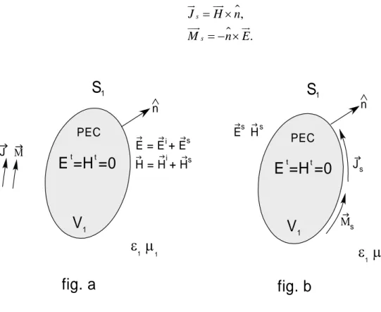
Let us now assume that the obstacle occupying region V is a perfect electric conductor. ₁

A medium with parameters ε_r and μ_r is outside and around V , and the sources ₁

1

J ur

,M1

uur

radiate in the presence of the conductor obstacle, as shown in figure 1.4 a. We

now need to determine the scattered fields Eurscatand uurHscat which, when added to E1

ur

and H1

uur

, will allow us to determine the total fields urE and Huur. To compute urEscat and

scat

H uur

outside V and ₁ Eur=Huur=0, total fields, inside V , the equivalent problem of fig 1.4 ₁ b is formed with equivalent sources

$ $ , . s s J H n M n E = × = − × ur uur uur ur (1.16) PEC

V

₁

E =H =0

t t

S

1

fig. a

J J ΜJ

ε μ

1 1 n H = H + HJ Ji Js E = E + E J J_i Js PEC

V

₁

E =H =0

t t

S

1

fig. b

ε μ

1 1 n ΜJ_s JJ_s J Hs EJs

The equivalent problem of fig 1.4 b states that the perturbed fields Eurscatand Huurscat scattered by the obstacles can be computed by placing equivalent currents (1.16) along the boundary of the scattering body and radiating in its presence. Since the target is made by PEC, the boundary conditions dictate that the tangential electric field must vanish on the PEC surface. It leads that equivalent sources are:

$, 0. s s J H n M = × = ur uur uur (1.17)

From equations (1.17) and equations (1.7), Eurscatand uurHscat can be expressed as

2 0 , . scat scat H A A k A E jωε = −∇× ∇∇ ⋅ + = − uur ur ur ur ur (1.18)

Now integral equations for the unknown equivalent sources can be formulated by combining the surface equivalent principle, the source field’s relationships (1.7) and the boundary conditions. Equations (1.5) may be combined with equations (1.18) to produce 2 0 ( ) ( ) , ( ) ( ) . inc inc A k A E r E r j H r H r A ωε ∇∇ ⋅ + = − = − ∇× ur ur ur ur uur uur ur (1.19)

At present, these relationships simply define the fields urE and Huur produced by the

excitation in the presence of the PEC. scatterer. If the boundary conditions on the electric field are imposed on the surface of the scatterer, the first equation of (1.19) becomes (mixed-potentials form)

$ $ 2 $

(

)

0 . inc A k A n E n n j A j

ωε

ω

⎫ ⎧∇∇⋅ + ⎪ ⎪ − × = ×_{⎨ ⎬}= × − − ∇ ⎪ ⎪ ⎩ ⎭

Φ

ur ur ur ur (1.20)

It is referred to as the electric field integral equation EFIE for the unknown equivalent

surface current density Js

ur

. It can be used to find this current at any point on the scatterer surface. It should be noted that (1.20) is an integro-differential equation but usually it is referred to as an integral equation. The EFIE is an equation of the first kind

because the unknowns Js

ur

occur only within the integral present in the convolution of

(1.11) for finding the vector potential Aur .

If the boundary conditions are applied on the second equation of (1.19) it leads to the magnetic field integral equations MFIE

$ inc s

{

$

}

. S n H J n A + ×uur =ur − ×∇×ur (1.21)

It is also an integro-differential equation for the unknown surface current Js

ur

and it is

enforced an infinitesimal distance outside the scatterer surface (S+). The MFIE is an

integral equation of the second kind because the unknown current Js

ur

occurs by itself and within the integral. Other integral equation is the combined field integral equation CFIE, which is a combination of the MFIE and EFIE.

1.3.2 PMCHW for homogeneous lossy dielectric objects

In the case of a homogeneous dielectric region a set of four integral equations can

be formulated to calculate the electric and magnetic fields urE and Huurin terms of

equivalent electric and magnetic currents Jur and Muur on the surface of the object. The

equation to calculate the electric current is the Electric Field Integral Equation (EFIE) and there are two such equations: one is for the field outside the object (EFIE-O) and the other is for the field inside the object (EFIE-I). The equation to calculate the magnetic current is the Magnetic Field Integral Equation (MFIE) and there are also two

such equations: one is for the field outside the object (MFIE-O) and the other is for the field inside the object (MFIE-I). Since we are dealing with four equations and two

unknowns, it is possible to develop a number of different formulations to solve for Jur

and Muur. Unfortunately, most of these formulations suffer from non-uniqueness of their

solution at frequencies associated with internal cavity resonances for a conducting object. This problem is particularly evident for large objects because it is easier to hit a resonance frequency. A formulation to remedy this defect is obtained by linearly combing EFIE and MFIE linearly to form the so called Combined Field Integral Equation (CFIE). Another formulation, which is widely used for scattering by 3-D dielectric bodies, is the so called Poggio, Miller, Chang, Harrington, and Wu (PMCHW) [8]. In this formulation, the EFIE for the field outside the object is combined with the EFIE inside the object to form a combined equation (EFIE-I + EFIE-O). Similarly, the MFIE inside and outside the object are combined in the same way (MFIE-I + MFIE-O). This specific formulation is found to be free from interior resonances and yields accurate and stable solutions.

Let us consider the problem of electromagnetic scattering by an arbitrarily shaped

and homogeneous body characterized by a permittivity

ε

₂ and permeability

μ

₂ and

embedded in an infinite and homogeneous medium having a permittivity ε1 and

permeability μ₁, as shown in fig. 1.5. The permittivity and permeability can be

Einc Hinc (ε1μ1) Region R1 Region R2 (ε2μ2) n1 n2 E1=Einc+Es H1=Hinc+Hs E2,H2

Fig. 1.5 Original problem: electromagnetic scattering from dielectric body

n1 Null Field J1 M1 Region R1 S1 (ε1,μ1) (ε1,μ1)

Fig. 1.7 Equivalent sub-problem: equivalence in the exterior region R ₂

constitutive parameters

ε

₁and

μ

₁; R₂ is the interior dielectric region characterized by

2

ε

and

μ

₂.The total electric and magnetic fields in region R are denoted by _i Euuv_iand uuvH_i , respectively, and Euv uuvinc,Hinc, ,E Hsi is

uv uuv

denote the incident and scattered fields in region i,

respectively. The normal vector $n points into the region i R_i , and S₁ denotes the

boundary surface between R and ₁ R . ₂

By applying the equivalence principle, we can derive two equivalent sub-problems shown in fig. 1.6 and fig. 1.7. The first sub-problem (Fig. 1.6) is

electromagnetically equivalent to the original problem in region R₁ (Fig. 1.5), whereas

the second is equivalent to the original problem in region R2 .The equivalent electric

and magnetic current densities are defined as (1.17).

In the null field regions, the constitutive parameters are the same as in the non-null field region, so the equivalent currents radiate into an unbounded homogeneous medium. The two sub-problems can be related to each other by enforcing the boundary conditions on the fields that must be satisfied in the original problem of fig. 1.5.

Specifically, the tangential components of the electric and magnetic fields must be continuous across the surface S . Since $₁ n2= − on Sn$1 1, this implies:

1 1 1 1 2 1 2 1 S S S S J J J M M M = − = = − = uuv uuv uv

uuuv uuuv uuv (1.22)

For each equivalent representation, scattered fields radiated by the equivalent and magnetic currents can be expressed in mixed-potentials form as following: .

for region R : ₁ ( ) ( ) ( ) ( ) ( ) ( ) ( ) ( ) 1 1 1 ' 1 1 1 1 1 1 1 1 1 s s r r r r r r r r E j A F H j F A

ω

ε

ω

μ

= − − ∇Φ − ∇× = − − ∇Ψ + ∇× v v v v v v v v

uuv uuv uuv

uuv uuv uuv (1.23)

for region R : ₂ ( ) ( ) ( ) ( ) ( ) ( ) ( ) ( ) 2 2 2 ' 2 2 2 2 2 2 2 1 1 s s r r r r r r r r E j A F H j F A

ω

ε

ω

μ

= + ∇Φ + ∇× = + ∇Ψ − ∇× v v v v v v v v

uuv uuv uuv

uuv uuv uuv (1.24)

Where ( ) ( ) ( ) ( ) ( ) ' ' ' ' ' ' ' ' ' , ' 1 1 1 ' i i i i i e s m s jk r r i i i i r r r r r r j J j M j e G r r k

σ

ε

ε

ωε

ρ

ω

ρ

ω

ω μ ε

− − ⎡ ⎤ = _⎢ − _⎥ ⎣ ⎦ ⎡ ⎤ = − _⎣∇ ⋅ _⎦ ⎡ ⎤ = − _⎣∇ ⋅ _⎦ = − = v v v v v v v v uv uuv v v (1.25)

On enforcing the boundary condition that the total tangential electric and magnetic fields across the surface of the arbitrary dielectric scatterer, the following combined

field integral equations are obtained in terms of the unknown surface equivalent electric and magnetic currents:

( ) ( )

[

( ) ( )

]

( ) ( ) ( ) ( )

[

( ) ( )

]

( ) ( ) 1 2 1 2 1 2 ' ' tan 1 2 tan 1 2 1 2 1 2 tan 1 2 tan inc inc r r r r r r r r r r r r F F E j A A A A H j F F ω ε ε ω μ μ = + + ∇Φ + ∇Φ + ∇ × + = + + ∇Ψ + ∇Ψ − ∇ × + ⎧ _{⎡ ⎤} ⎡ ⎤⎫ ⎨ _{⎣ ⎦ ⎢ ⎥}⎬ ⎩ ⎣ ⎦⎭ ⎧ _{⎡ ⎤} ⎡ ⎤⎫ ⎨ _{⎣ ⎦ ⎢ ⎥}⎬ ⎩ ⎣ ⎦⎭ v v v v v v v v v v v v v v v uv uv uv uv uv v v (1.26)

Equations (1.26) are well known as PMCHW formulation, which is widely used to treat scattering problem by dielectric objects.

1.3.3 Multilayered Green’s function

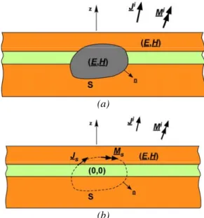
In the case of Multilayered Medium the first step is to correctly formulate the integral equation for the situation presented in Fig. 1.8 (a), where known electrical and

magnetic currents (J i, M i) are radiating an arbitrary shaped object embedded in this

medium. An external equivalent problem is shown in Fig. 1.8 (b) where the same

impressed currents (J i, M i), together with surface currents (Js, Ms) produce the correct

fields (E, H) exterior to S and null fields inside S.

Since (E, H) = (E i+E s, H i+H s), where (E i, H i) are the impressed fields due to (J i, M i)

and (E s, H s) are the scattered fields due to (Js, M s). The boundary conditions at S

impose that:

(

i s[ , ]

)

s s s S M = − ×n E +E J M ₊ (1.27)

(

i s[ , _s]

)

s s S J = ×n H +H J M ₊ (1.28)

(a)

(b)

Fig. 1.8 - Object in a multilayered medium excited by known electric and magnetic currents. (a) Original physical configuration; (b) External equivalent problem.

where n is the outward unit vector normal to S and the subscript S+ indicates that the

fields are evaluated as the observation point approaches S from the exterior region. If the media is linear, we can express the fields produced by an arbitrary current distribution (J, M) as ; ; EJ EM E = G J + G M (1.29) ; ; HJ HM H = G J + G M (1.30)

where G PQ(r|r’) is the DGF relating P-type fields at r Q-type currents r’. Since the

DGF’s for the layered medium of Fig.1(b) are available, one can use (1.29) and (1.30) to compute the impressed fields and to express the scattered fields in (1.27) and (1.28)

in terms of the unknown currents (Js, M s). In view of the hypersingular behavior of

EJ

G and GHM, it is preferable to convert (1.29) and (1.30) into their mixed-potential

forms before they are used in (1.27) and (1.28). However, since in layered media the scalar potential kernels associated with the horizontal and vertical current components

are in general different, in the method presented in [19] the scalar potential kernel have been modified for arbitrary current distributions and the final mixed-potential forms are

(

'

)

0 0 1 ; , ; ; A EM E j G J K J C z J G M j φ φ

ωμ

ωε

= − + ∇ ∇ ⋅ + $ + (1.31)

(

'

)

0 0 1 ; ; , ; HJ F H G J j G M K M C z M j φ ψ

ωε

ωμ

= − + ∇ ∇ ⋅ + (1.32)

where the prime over the operator nabla indicates that the derivatives are with respect to

the source coordinates. In addition, G A and G F are the DGF’s for the magnetic and

electric vector potentials, respectively, KΦ and KΨ are the corresponding scalar kernels,

and CΦ and CΨ are the correction factor which are associated with the longitudinal

electric and magnetic currents, respectively. It is worth of notice that the two divergences are proportional to, respectively, the electric and magnetic charge densities.

By using the mixed-potential representation given by the (1.31) and (1.32) in

(1.27) and (1.28) we are able to express the scattered fields radiated by (Js, M s) in

terms of the MPIE’s. Since the only difference with respect to the free space case is the dyadic nature of the vector potential kernels, these MPIE’s can be employed in the same numerical solution procedures developed for the free space case.

1.4 RADAR CROSS SECTION

Radar cross section is a measure of the power that is returned or scattered in a given direction, normalized with respect to the power density of the incident field. The purpose of this normalization is to arrive at a description that is independent of the distance between the target and antenna or source. Generally, the receiver of the scattered energy is assumed to be located far enough from the target so that the target is essentially a point scatterer. This implies that the distance of the target is much longer

than any significant target dimension. This “point scatterer” radiates energy isotropically. The definition of the radar cross section is based upon this concept of isotropic scattering, assuming that the target is illuminated by a plane wave.

Formally, the radar cross section is

2 2 2 lim 4 . scat r inc E r E

σ

π

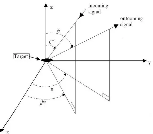
→∞ = ur ur (1.33)

The limit is presented because it is supposed to have a plane wave and the target is assumed to be a point scatterer. When an object is illuminated by an electromagnetic wave, energy is dispersed in all directions. The spatial distribution of energy depends on the size, shape, and composition of the scattering body, and on the frequency and nature of the incident wave. For a given object, the radar cross section is a function of the angle of incident wave and of the angle to the observation point. The convention

adopted is that the angles

ϑ

inc and

φ

inc define the direction of propagation of the

incident field and the angles

ϑ

,

φ

define the direction of propagation of the scattered

field of interest. This coordinate system is illustrated in fig 1.9.

The case where

ϑ

inc =

ϑ

and

φ

inc = is called monostatic scattering. When the

φ

observation point and the direction of incident wave are clearly separated,

ϑ

inc ≠

ϑ

and

inc

φ

≠ , the bistatic radar cross section is observed. The bistatic radar cross section is

φ

a useful characterization of the scattering properties of an electromagnetic target. It is defined as the area that, if multiplied by the power flux density of the incident field, yields sufficient power to produce by isotropic radiation the same intensity in a given direction as that actually produced by the scatterer.

For a three dimensional geometry where all components of the magnetic and electric field are present, the bistatic scattering cross section can be expressed for plane wave incidence as

(

)

(

)

(

)

2 2 2 , , , , lim 4 . , scat inc inc

r inc _{inc inc}

E r E

ϑ φ

σ ϑ φ ϑ φ

π

ϑ φ

→∞ = ur ur (1.34)

In the far zone, the scattered electric field has the form

$ $ _.

scat scat scat

E ≅

ϑ

Eϑ +

φ

Eφ

ur ur ur

(1.35)

since equation (1.35) involves the expression

2 2 2

,

scat scat scat

E ≅ Eϑ + Eφ

ur ur ur

(1.36)

it is sufficient to compute the ϑ and

φ

components separately. Consequently, the

scattering cross section can be written as

(

, , inc, inc

)

(

,

)

(

,

)

, ϑ φ

σ ϑ φ ϑ φ

=

σ ϑ φ σ ϑ φ

+ (1.37) where

(

)

( )

( )

2 2 2 , , lim 4 , 0, 0 scat r inc E r E ϑ ϑ θ φ σ ϑ φ π →∞ = ur ur (1.38) and

(

)

( )

( )

2 2 2 , , lim 4 . 0, 0 scat r inc E r E φ φ θ φ σ ϑ φ π →∞ = ur ur (1.39)

As shown for emphasis in equation (1.37), σ is a function of the direction of the

incident field and the far zone observation angle. The bistatic scattering cross section is also a function of polarization of the incident wave. To explicitly characterize the scatterer as a function of polarizations, the scattering cross section data can be obtained for two orthogonal polarizations and arranged in the form of a scattering matrix such as

ϑϑ ϑφ φϑ φφ σ σ σ σ ⎡ ⎤ Σ = ⎢ ⎥ ⎣ ⎦ (1.40)

The entries of this 2 2× matrix remain a function of the direction of the incident