Chapter 5 DIESEL/GASOLINE DUAL FUEL COMBUSTION 5.1 INTRODUCTION

Chapter 5

DIESEL/GASOLINE DUAL FUEL COMBUSTION

5.1 INTRODUCTION

As aforesaid, the HCCI combustion process is able to combine the best features of gasoline SI and diesel CI engines. As in SI engines, fuel and air are homogeneously mixed, yet, as in CI engines, combustion is primed by the high compression-induced temperature. Instantaneous volumetric combustion is avoided, which would damage the engines, with suitable solutions and typically high EGR levels. The well-mixed charge prevents fuel-rich diffusion combustion reducing particulate emissions and eliminating the high-temperature flames typical of SI engine combustion, which reduces NOx emissions. In addition, HCCI combustion can provide diesel-like fuel efficiency [21].

However, since HCCI combustion is achieved through the auto-ignition of a homogeneous mixture around TDC, it is more challenging to control the start of combustion times and the rate of heat release for this combustion mode than for conventional engines that have direct control of combustion initiation (spark for SI engines and fuel injection for diesel engines). In addition, the increase in cycle-to-cycle variation caused by the ignition timing uncertainty leads to uneven engine operation.

As a way to solve the combustion phasing control problem, diesel/gasoline dual-fuel combustion is explored in this study. A small amount of diesel fuel is injected as a pilot injection to ignite a pre-mixture of gasoline (or other high-octane fuel) and air. Although dual-fuel combustion is an attractive way to achieve controllable HCCI operation, relatively few studies [88, 89] are available to help in understanding its in-cylinder combustion behavior.

This study describes a numerical study of diesel-gasoline dual-fuel combustion, to understand the influence of fuel mixture composition and injection timing on combustion behavior. Two different injectors were considered in the simulations and their effects on mixture formation are shown.

A primary analysis was performed to investigate the feasibility of the concept using the KIVA 3V code with a modified version of the Shell-CTC combustion model, that requires small computational resources. Then, an accurate numerical analysis was performed using the KIVA 3V code, integrated with CHEMKIN and G-equation combustion models in order to understand the influence of fuel mixture composition and injection timing on dual-fuel combustion behavior in several load and engine speed conditions. Four different combustion strategies, with different calculation approaches in the burning zone, have been used for this study to test their predictability. Available experimental data have been used to validate a new

combustion strategy proposed in this study before proceeding with the dual-fuel analysis.

5.2. NUMERICAL

APPROACH

Basically the same code settings described in the previous chapter have been used in this research activity. The hybrid Kelvin Helmholtz–Rayleigh Taylor (KH-RT) model was used for describing diesel high-pressure spray breakup and injection process. Several autoignition and combustion models, like Shell-CTC model, detailed chemistry using CHEMKIN and G-Equation flame mode, have been used in this study. However, for this study, some numerical settings were necessary and several combustion calculation approaches have been tested. Further details are given below.

5.2.1. SHELL-CTC MODEL SETTINGS FOR DUAL FUEL COMBUSTION

The Shell-CTC combustion model has been used for preliminary concept validation of dual fuel combustion, due to its low computational time cost. However, to apply this model to dual-fuel combustion, some model modifications are needed. Previous research by Kong et al. [88] and Singh et al. [89] used fixed model parameters for the injected diesel fuel only. But, in the present study, the effect of the relative composition of diesel and gasoline in the local charge mixture were considered by adjusting the combustion model constants as a function of the diesel/gasoline proportion. In this way, the two original fuels can be treated as a single fuel for modeling ignition and combustion processes in each computational cell (average properties of the composition are used in relevant calculations). The remaining fuel after the calculation is then re-distributed to both the diesel and gasoline fuels according to their initial proportions at the beginning of the combustion calculation. Note that the relative consumption rates of diesel and gasoline fuels are assumed to be the same.

When the Shell-CTC model is activated, a NOx model [52] based on the extended Zeldovich reactions is used. Soot emissions are predicted by a phenomenological soot model that uses competing formation and oxidation rates. The formation is described by the Nagle-Strickland-Constable (NSC) oxidation model [85]. The parent fuel molecule is used as the species from which the soot forms.

5.2.2. DUAL-FUEL COMBUSTION USING DETAILED CHEMISTRY AND FLAME PROPAGATION APPROACH

The currently used version of the KIVA3V code is also integrated with CHEMKIN detailed chemistry solver and G-equation combustion model. These two models are combined to work together as described in the following strategy proposed by Singh et al. [19]:

• During the simulation CHEMKIN is used to account for the detailed chemical kinetics of combustion, and the code checks whether a single or multiple ignition kernels are appearing in every computational cell of the combustion chamber.

• Once an ignition kernel appears, a G isosurface is initialized from the G-equation model as a contour of the burning zone. During the simulation the G surface follows the expansion and the growth of the burning zone. • The CHEMKIN model keeps checking both the burnt and the unburnt

zones to account for termination reactions and to capture eventual new ignition kernel appearances.

To account for species change within the burning region, defined by the G isosurface, several calculation strategies have been considered in this study in order to test their predictability for dual-fuel combustion.

Chemistry approach - In this approach detailed chemistry using CHEMKIN is

used for the combustion calculation within the burning region. From a global point of view, this approach is similar to a pure detailed chemistry calculation in which the CHEMKIN solver is used for autoignition and combustion calculations in the whole computational domain.

G-equation approach - In this second approach the G-equation flame model is

used to account for chemical species change in the burning region.

High Energy approach - In this third approach both the CHEMKIN and G-equation

approaches are used to calculate the internal energy in every computational cell in the burning region. Then, the model predicting the higher cell internal energy is used to update the chemical species density and internal energy. This approach is the same as the Hybrid combustion model already validated against experimental data by Singh et al. [19].

Damkohler approach - In this strategy a new criterion is used to choose between

the CHEMKIN and G-Equation models in the burning region. A Damkohler number is introduced as a ratio between a laminar flame propagation timescale and a chemical timescale. The time scales are used to evaluate, for every computational cell in the burning region, whether combustion could be locally controlled by flame propagation or by volumetric heat release. The Damkohler equation is defined as

,

chem lam

Da

τ

τ

=

(5.1)

where

τ

_lam and

τ

_chem representing the laminar and chemical timescale respectively can be defined as

,

2 l l l l lam

S

S

D

δ

τ

=

=

(5.2)

[

]

[

]

dt

Fuel

d

Fuel

chem

=

τ

(5.3)

where

D

_l is the laminar diffusivity,

S

_l is the laminar flame speed,

δ

_l is the flame thickness and [Fuel] is the effective fuel concentration (sum of premixed gasoline and injected diesel). Note that the use of the laminar time scale (based on laminar flame speed and diffusivity) is consistent with the interpretation that at a subgrid level flamelets control the combustion rate. In the case that flame propagation is dominant, with a bigger chemical timescale, the G-Equation model is used for the combustion calculation in that cell. Otherwise, with a bigger laminar timescale, CHEMKIN is adopted to compute the combustion rate and energy release.

For more realistic combustion modeling, the MIT PRF n-heptane/iso-octane mechanism with 32 species and 55 reactions [54] was used for dual-fuel combustion simulation with detailed chemistry. N-heptane and iso-octane, present in the mechanism, were assumed as surrogates for diesel and gasoline fuel for dual-fuel application. For the NOx emission calculations, a simplified NOx formation model consisting of 4 species and 9 reactions was obtained from the GRI mechanism [56] and added to the PRF mechanism. The Hiroyasu soot model [90] was used with the detailed kinetics calculation. As aforesaid, the PRF mechanism coupled with the NOx formation reactions was used in this work, and is given in

Appendix A.

Though n-heptane combustion chemistry can adequately predict diesel combustion characteristics, it is well known that the physical properties of n-heptane are very different from those of diesel fuel (e.g., density, distillation curve). Since the physical properties of heavier hydrocarbons (dodecane, tetradecane, hexadecane, etc.) are more similar to diesel properties, tetradecane properties were used to model the diesel injection, breakup and evaporation processes for the dual-fuel investigation, as has been done in numerous previous studies.

5.3. PRELIMINARY CONCEPT VALIDATION

Diesel/gasoline dual-fuel combustion was simulated using a modified version of the Shell-CTC model in order to test the capability of this new approach of controlling combustion phasing while maintaining low levels of pollutant emissions. One of the HCCI cases described in Chapter 4 was taken as a baseline case with 0% diesel and 100% gasoline, then the relative amount of the two fuels was changed while keeping the total energy released constant. For all the cases

Table 5.1. Dual-fuel combustion operating conditions.

% of Gasoline 25 50 65 75 80 85 90 95 98

Gasoline premixed (g) 0.011 0.023 0.030 0.035 0.037 0.039 0.042 0.044 0.046

Diesel injected (g) 0.033 0.022 0.016 0.011 0.009 0.007 0.004 0.002 0.001

Injection duration (ca) 3.7 2.47 1.735 1.23 0.991 0.744 0.49 0.24 0.099

Injector type Conventional Diesel Multi hole injector with eight equally-spaced holes

Injection pressure (MPa) 150 Injection timing (ca ATDC) -6

IVC temperature (˚K) 391 IVC press (MPa) 0,11 Engine Speed (rev/min) 700

considered in the study, the gasoline fuel was considered to be premixed with air at IVC time, and the diesel fuel was injected into the combustion chamber during the compression stroke. The major operating conditions are summarized in Table 5.1. The reference engine is the Caterpillar 3401 SCOTE engine already described in Chapter 4. The engine specifications were reported in Table 4.2.

The piston geometry and computational grid used for this simulation are shown in Fig. 5.1. A 45˚ sector mesh was used in this study, considering that the diesel injector used had eight equally-spaced nozzle holes. All major geometric dimensions of the experimental combustion chamber, including bore, stroke, bowl volume and squish height were replicated in the computational grid. The mesh was composed of about 22,000 computational cells at BDC with an average cell size of 2.0 x 2.3 mm in the radial and vertical directions, respectively, for the bowl region. The chosen mesh size represents a compromise between computational time and accuracy, but was found to give adequately grid independent results.

For the Shell-CTC model both of the fuels were considered in the auto-ignition calculation as expected for HCCI combustion. Since this is not a conventional combustion strategy, the combustion model constants had to be tuned in order to match the ignition delay and the main apparent heat release rate as discussed below.

Figure 5.1. Computational grid for dual-fuel simulation.

5.3.1. PRELIMINARY DIESEL CASE VALIDATION

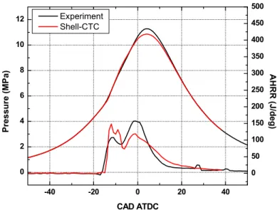
Before starting the dual-fuel combustion study a simple diesel case was simulated in order to test the modified Shell-CTC code against experimental data. The operating conditions [89] are summarized in Table 5.2. For this operation the engine compression ratio was reduced from 16:1 to 14.5:1. In Fig. 5.2 a comparison in terms of pressure and heat release rate is reported for the sample diesel case. The modified Shell-CTC model predict the in-cylinder gas pressure and apparent heat release rates reasonably well, though the model over-predicts the apparent heat release rate at the time of ignition.

Table 5.2. Experimental operating conditions for diesel test case [14].

Engine Type Caterpillar 3401 Fuel injected 0.093 g (High Load)

Compression ratio 14.5:1 Injection timing -22 ca ATDC

Displacement 2.43 L Engine Speed 1693 rev/min

Bore X Stroke 13.7 X 16.5 cm Combustion Chamber Bowl in Piston

Fuel Injection Direct injection Intake P 0,181 MPa

Injection type Pencil-type, six hole

nozzle Intake T 348 ˚K -40 -20 0 20 40 0 2 4 6 8 10 12 Experiment Shell-CTC CAD ATDC Pres sure (MP a ) 0 50 100 150 200 250 300 350 400 450 500 AH RR ( J/d eg )

Figure 5.2. Pressure and apparent heat release rate for sample diesel case.

5.3.2. PRELIMINARY DUAL FUEL SIMULATIONS

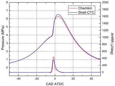
After this initial diesel test the dual-fuel combustion cases were simulated using Shell-CTC model. Pressure profiles and apparent heat release rate results for only two different relative fuel mixture compositions are reported in Figs. 5.3 and 5.4. Since no experimental measurements are available at this time, the proposed simulations were repeated using pure detailed chemistry calculation with CHEMKIN. The Shell-CTC model constants were tuned in order to match the detailed chemistry results for every proposed fuel mixture compositions.

-40 -20 0 20 40 0 1 2 3 4 5 6 7 8 0 200 400 600 800 1000 1200 1400 1600 1800 2000 P ressure (M Pa) CAD ATDC Chemkin Shell-CTC A HRR ( J/d eg )

Figure 5.3. Pressure and apparent heat release rate for 25% of gasoline case.

-40 -20 0 20 40 0 1 2 3 4 5 6 7 8 0 200 400 600 800 1000 1200 1400 1600 1800 2000 Pres su re (M Pa) CAD ATDC Chemkin Shell-CTC A H RR (J /d eg)

Figure 5.4. Pressure and apparent heat release rate for 95% of gasoline case. 61

For a fixed injection timing of diesel fuel, the variation of the diesel/gasoline proportion is seen to change the ignition timing of the mixture, which indicates ignition timing controllability of the dual-fuel operation.

With the detailed chemistry model results as a reference, adjustment of two representative model constants (Af04, pre-exponential values of one of the chain propagating reactions in the Shell ignition model and the rate determining reactions in the CTC model, A in Eq. 3.34) as a function of diesel/gasoline proportion was obtained. Figure 5.5 shows the correlations for the two model constants with respect to gasoline percentage in the total energy contents. These correlations were employed in the simulation of the cases of interest.

0 20 40 60 80 100 120 10 15 20 25 30 0.00 0.05 0.10 0.15 0.20 0.25 0.30 0.35 0.40 0.45 0.50 Parabola Y =29.99157-0.43569 X+0.00214 X2 af04 Af 04 (*e+ 4) %Gasoline A Exponential Equation: y = A1*exp(-x/t1) + y0 y0 0.52004 A1 -0.04504 t1 -47.08205 A ( *e+9)

Figure 5.5. Shell-CTC model constants correlation.

In Fig. 5.6, NOx and soot emission prediction (at EVO) for various amounts of the two fuels is provided. The emissions were normalized with the maximum value among the cases considered here. As expected, increasing the percentage of premixed gasoline caused both soot and NOx emissions to decrease. The decreased amount of injected diesel allows the mixture to become closer to a homogeneous mixture, which lowers the local burned gas temperatures and, consequently, reduces the soot and NOx emissions.

The results show that the modified (and tuned) Shell-CTC could be a useful tool for dual-fuel combustion calculations due to its low computational time cost compared to detailed chemistry. However, from the previous chapter’s results, it appears that the present model is not very accurate on predicting emission production. Therefore, for a more accurate investigation, detailed chemistry based model was chosen for the continuation of this research.

20 30 40 50 60 70 80 90 100 0.0 0.2 0.4 0.6 0.8 1.0 0.0 0.2 0.4 0.6 0.8 1.0 soot Nor m alized soot em iss ion % of Gasoline N or m a lized NO x _em is sion NO_x

Figure 5.6. NOx and soot dual-fuel predictions using the CTC model.

5.4. DAMKOHLER COMBUSTION STRATEGY VALIDATION

Before proceeding with the dual-fuel analysis, some model validation for the proposed Damkohler combustion strategy was necessary.

Available measurement of diesel liftoff length [20] and diesel/natural gas dual-fuel combustion experiments [19] were used for the validation of the code in order to test the reliability of the proposed combustion strategy. Details are reported below.

5.4.1. DIESEL LIFTOFF LENGTH VALIDATION

The first validation was performed against some Sandia diesel flame liftoff experiments. Before proceeding a brief introduction regarding the diesel flame conceptual model proposed by Dec is reported.

5.4.1.1. Conceptual Model of Conventional Diesel Spray Combustion

Various conceptual models are proposed in the literature to describe spray combustion. The knowledge provided by observations from optical techniques such as laser-induced fluorescence (LIF), laser-induced incandescence (LII) of soot, and other laser-light scattering diagnostics has been very useful in understanding spray combustion. Based on observations of in-cylinder phenomena from multiple optical diagnostics, several researchers have proposed conceptual models for conventional diesel combustion processes, including Dec (1997) [91]. The Dec proposed model is shown in Figure 5.7.

Figure 5.7. General scheme of the diesel combustion proposed by Dec(1997) [91].

Figure 5.7 shows that the air entrainment vaporizes all the liquid-fuel within a distance of around 20 mm downstream from the injector. No liquid was observed in the combustion zone. A short distance downstream, the vapor-fuel and entrained air have mixed to form a uniform mixture, and a standing fuel-rich premixed flame exists just downstream of the uniform fuel air mixture. Then next to this premixed-rich flame soot appears as small particles. The soot concentration and particle size increase towards the head vortex at the tip of the jet, with the highest soot concentration and largest soot particles in the head vortex. Also, soot is distributed throughout the jet cross-section of the downstream portion of the jet. The diffusion flame exists at the periphery of the jet, surrounding the soot-producing region. The flame extends back toward the injector to a point just upstream of the tip of the liquid-fuel penetration. The distance from this point to the injector tip is defined as liftoff length. The NOx emissions are also produced at the periphery of the jet in the vicinity of the diffusion flame where the maximum combustion temperature is achieved.

5.4.1.2. Validation with SANDIA Liftoff Experiments

In this section, the KIVA3V code implemented with the new Damkohler combustion approach was validated against the Sandia diesel flame liftoff experiments.

Nine different test cases were selected from Picket et al. (2005), as shown in Table 5.3. The first two cases have different ambient gas density (ρamb). Cases 3 and 4 were selected to evaluate the effect of ambient gas temperature (Tamb). For cases 5 and 6, different ambient oxygen concentration, (O2)amb, was proposed. All of the first 6 cases have the same injector nozzle diameter (Dnoz), rail pressure (Prail), and fuel temperature (Tfuel). Cases 7 and 8 were selected with different injector nozzle diameters. Finally, Case 9 was selected to investigate the effect of fuel temperature on liftoff length.

Table 5.3. Liftoff Length Test Matrix.

C1 C2 C3 C4 C5 C6 C7 C8 C9 ρamb (kg/m3) 14.8 30.0 14.8 14.8 14.8 14.8 14.8 14.8 14.8 Tamb (K) 900 900 800 1000 900 900 900 900 900 (O2)amb(%) 21 21 21 21 19 15 21 21 21 Dnoz(µm) 180 180 180 180 180 180 100 246 180 Prail (bar) 1380 1380 1380 1380 1380 1380 1380 1380 1380 Tfuel(K) 436 436 436 436 436 436 436 436 373

The computational mesh representing the Sandia cubical combustion vessel is shown in Figure 5.8. Each side of the cube is 10.8 cm in length. The mesh is composed of about 175,000 computational cells. It has the highest resolution near the center axis, with cell size of 1.0 x 1.0 x 1.55 mm, and the lowest resolution on the outer edges, with cell size of 2.35 x 2.35 x 1.5 mm. The diesel injector is located on top, along the central axis.

The simulations were started at time t = 0 with a uniform mixture distribution in the combustion chamber. The swirl and other velocity components were initialized to zero and small values of the turbulent kinetic energy and length scale were assumed at the start of computations. The gas pressure and temperature were initialized based on the experimental measurements. A top-hat injection rate-shape was assumed, consistent with that used in the experiments (Pickett et al., 2005) [20].

Figure 5.8. 3-D computational mesh of the Sandia vessel.

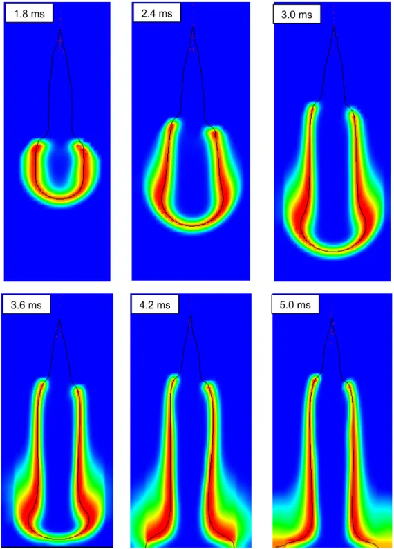
Figure 5.9 shows the KIVA3V predictions of OH radical distribution at various times during the jet development for Case 3 (C3, lower Tamb) in Table 5.3. As expected, the OH radical concentration is highest along the stoichiometric equivalence ratio line (black-colored line). The OH radical concentration can also be used to mark the location of flame liftoff. Indeed, Pickett et al. (2005) [20] used OH chemiluminescence to measure the flame liftoff location. In their measurements, they called the distance between the injector tip and the first location with detectable OH radicals the flame liftoff length. The same methodology was adopted in this study to measure the flame liftoff length from OH radical images predicted by the model. In Fig. 5.10 typical diesel triple flame structure is shown and briefly described in order to show the capability of the code to predict diffusive combustion. Transient liftoff measurements corresponding to the images in Figure 5.9 are shown in Fig. 5.11. As time progresses, the flame moves in an upstream direction towards the injector. The initial movement of flame is faster, then the slope of the curve decreases and does not change from about 4.0 to 5.0 ms, indicating that a steady flame liftoff length has been established. Considering this, all the simulations were run only up to 5 ms and the steady-state flame liftoff lengths at the end of the calculations are presented.

Figure 5.12 shows numerical steady liftoff length predictions for all nine cases listed in Table 5.3. The results show that the model gives accurate predictions of the dependence of liftoff length on many controlling parameters, including the ambient gas density, ambient temperature, ambient oxygen concentration, nozzle diameter, and the fuel temperature. However, the magnitude of the predicted liftoff length will also depend on the chemistry mechanism used.

Figure 5.9. OH radical distribution during the transient period of flame liftoff. The

number in the upper corner of each image is time after start of injection (SOI). 2.4 ms 1.8 ms 3.0 ms 5.0 ms 4.2 ms 3.6 ms 67

Figure 5.10. Predicted diesel triple flame structure.

Figure 5.10 shows numerically predicted diesel triple flame structure. The image shows the OH radical distribution in a plane along the fuel-jet-axis and the stoichiometric mixture.

The inset image shows the region of the flame near the liftoff location. The region where the flame intersects the Phi = 1 line is called the stoichiometric branch. The part to the right side of the high concentration OH region represents the fuel-lean and part on the right side represents the fuel-rich branch. Fuel from the side of fuel-rich branch and oxidizer from the side of fuel-lean branch meet at the Phi = 1 line where the diffusion flame is established. It clearly appears from the figure how the highest OH concentration follows the stoichiometric line. Most of the fuel chemical energy is released in the diffusion flame.

In Fig. 5.12 the transient liftoff length of all the nine cases of Table 5.3 are reported in order to analyze the influence of the changed operating conditions on the liftoff appearance and variation.

0 1 2 3 4 5 30 35 40 45 50 55 60 Case 3 Damkohler Li ftOff Length (m m) Time (ms)

Figure 5.11. Liftoff length transient variation for Case 3.

C1 C2 C3 C4 C5 C6 C7 C8 C9 0 10 20 30 40 50 60 70 Experiment DAMKOHLER S teady Lif to ff Lengt h (m m) Cases

Figure 5.12. Steady liftoff length results.

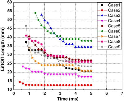
0 1 2 3 4 5 6 7 10 15 20 25 30 35 40 45 50 55 60 Case1 Case2 Case3 Case4 Case5 Case6 Case7 Case8 Case9 Lift Off Len g th (mm) Time (ms)

Figure 5.13. Transient liftoff length for all the nine cases proposed.

From Fig. 5.13 it can be observed how the liftoff flame for cases from 2 to 9 differentiates from the baseline case (case1). For case 2 and case 4, increasing ambient density or temperature, leads to the obtaining of a relatively small liftoff length, meaning that faster combustion occurs close to the injector tip. Oppositely, for cases 3 and 6, with lower temperature and lower O2 concentration, respectively,

a late combustion initiation gives high liftoff length. As expected case 5, with O2 concentration in between of Case 1 and Case 6, gives results in between of Case 1 and Case 6. Changing the nozzle diameter has a moderate effect of the liftoff length. Compared to case1, case7, with smaller nozzle diameter, leads to a faster combustion closer to the tip, probably due to fast droplets velocity and evaporation. On the other hand, case 8, features late combustion. Finally, decreasing the fuel temperature, as in case 9, causes higher liftoff length, due to the higher time necessary for fuel evaporation and mixing.

It emerges that also the slope of the curves is influenced by the start of combustion. For case 2, burning almost immediately after the injection, the slope of the curve is the smallest. On the other hand, while going towards late combustion, as in cases 3 and 6, a higher slope can be found.

5.4.2. VALIDATION WITH CUMMINS DIESEL/NATURAL GAS DUALFUEL EXPERIMENTS

Available experiments [19] regarding diesel/natural gas dual-fuel combustion were used as a comparison for the KIVA3V predictions with the Damkohler model selection strategy.

5.4.2.1. Reference Engine

The engine used for the experimental test was a six-cylinder, four-stroke, direct-injection Cummins diesel engine. Engine and injector specifications are listed in Table 5.4.

Table 5.4. Engine and injector specifications for diesel/natural gas combustion.

Engine type Cummins, DI Diesel

Number of cylinders 6

Bore x Stroke, cm 15.875 x 15.875

Displacement, L 20.23

Connecting rod length, cm 28.971 Geometric compression ratio 14.5:1

Fuel injector type Common rail Number of holes 4, equally spaced

Spray included angle 90°

Rail pressure, bar 1000

Nozzle diameter, mm 0.144

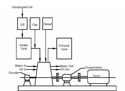
Figure 5.14. Schematic of the Cummins dual fuel engine setup.

Figure 5.14 shows the schematic of the engine setup. The primary engine fuel natural gas was injected into the intake manifold, and the secondary fuel diesel was injected directly into the engine cylinder. The engine was coupled with a dynamometer to maintain a constant speed of 1200 rev/min. All the tests were conducted at a brake power of 287 kW (BMEP = 1000 kPa).

5.4.2.2. Operating Conditions

Five different operating conditions were chosen for the Cummins diesel/natural-gas, dual-fuel engine. Table 5.5 lists some important characteristics of these operating conditions. As discussed above, the primary fuel, natural gas, was premixed into the intake port at an equivalence ratio of about 0.44. The diesel fuel was injected into the cylinder at a crank angle of -87° ATDC. The amount of diesel fuel injected and its injection duration was slightly different from every case. The intake temperature was kept constant at 333.5 K for all the five test cases, however, due to different amount of residual gas trapped and differences in its temperature, the temperature at intake valve closure (IVC) was slightly different. Note that the temperature for Case 5 is 16 degrees higher than the temperature for Case 1. The temperature and pressure at IVC were calculated using a commercial one-dimensional (1-D) cycle simulation code. The ERC skeletal reaction mechanism for n-heptane [55] with 30 species and 65 reactions simulated the diesel fuel chemistry. The skeletal mechanism retains the main features of detailed mechanisms and includes reactions of ketone hydrocarbons. The mechanism was validated using constant-volume ignition delay data and engine combustion experiments. While this reduced mechanism simulated the combustion reactions of the diesel fuel, the physical properties of the fuel, for use in the spray model, were taken as those of tetradecane. The ERC mechanism reaction pathway is reported in detail in Appendix B.

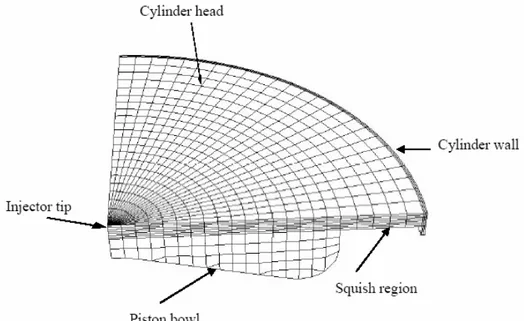
The piston geometry and computational grid used in the simulations are shown in Figure 5.15. The diesel injector had four equally-spaced nozzle holes, so the combustion chamber was represented by a 90º sector mesh with assumed periodic boundary conditions. The mesh was created using the standard KIVA-3V pre-processor. The mesh was composed of about 38,000 computational cells at bottom dead center (BDC).

Table 5.5. Test Matrix for Cummins dual fuel engine.

Tin(K) 333.5 333.5 333.5 333.5 333.5 TIVC(K) 392 397.5 403 405 408 PIVC(bar) 2.10 2.09 2.12 2.10 2.136 SOI (ATDC) -87 -87 -87 -87 -87 Qpilot (mg) 18.2 19 19 19.6 20 DOI (ca) 9.47 9.88 9.88 10.2 10.4 NG Phi 0.44 0.44 0.44 0.44 0.44 72

Figure 5.15. 90° sector computational grid at TDC for the Cummins

diesel/natural-gas, dual-fuel engine.

The computations were started from intake valve closure (IVC = -141° ATDC) with an assumed uniform distribution of natural gas and air mixture in the cylinder. The mass rate of injection profile for the diesel fuel was taken from the experimental measurements.

5.4.2.3. Diesel/Natural Gas Dual Fuel Combustion

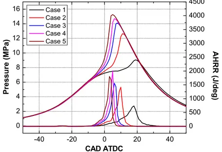
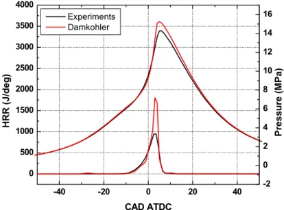
In Figs. 5.16 and 5.17 experimental and numerical pressure profiles and AHRR for all the five cases are proposed. Results in terms of pressure and heat release rate are reported in Fig. 5.18 for case 5.

From Case 1 to Case 5, the ignition delay slightly decreases and the rate of heat release strongly increases. Due to the earlier start of combustion, the peak cylinder pressure also increases. The increase in rate of heat release could be attributed to the increased mixture temperature at IVC (Table 5.5). Similar trends in ignition delay and rate of heat release are predicted by the simulations. However, there are some discrepancies between the experimental measurements and the model predictions. The model predicts higher rates of heat release, especially for cases 2 to 4. In this study, no tuning of the initial and boundary conditions and model constants was attempted to better match the burn rates for cases 2 to 4. It is noted that even seemingly slight inaccuracies in factors like the mixture initial conditions, diesel fuel spray distribution, flame speed, etc., could lead to such discrepancies in model predictions.

-40 -20 0 20 40 0 300 600 900 1200 1500 1800 Case 1 Case 2 Case 3 Case 4 Case 5 AHRR (J /de g ) CAD ATDC -2 0 2 4 6 8 10 12 14 16 Pr es sure ( M P a)

Figure 5.16. Experimental pressure profile and AHRR for all the proposed cases.

-40 -20 0 20 40 0 2 4 6 8 10 12 14 16 0 500 1000 1500 2000 2500 3000 3500 4000 4500 Pr es su re ( M P a) CAD ATDC Case 1 Case 2 Case 3 Case 4 Case 5 AHRR (J /deg)

Figure 5.17. Numerical pressure profile and AHRR for all the proposed cases.

In Fig. 5.19 a NOx emissions comparison between the simulations and experiments is reported for all the proposed cases. As it clearly appears from case 1 to case 5 the NOx emissions increases considerably, according to the previous considerations about pressure and heat release rate. Further on, the model predictions are able to follow reasonably well the experimental measurement.

-40 -20 0 20 40 0 500 1000 1500 2000 2500 3000 3500 4000 Experiments Damkohler H RR (J/d eg ) CAD ATDC -2 0 2 4 6 8 10 12 14 16 P res sure ( M P a)

Figure 5.18. Pressure profile and apparent heat release rate for case 5.

1 2 3 4 5 0.005 0.010 0.015 0.020 0.025 0.030 Experiment Damkohler NO x em iss ion s (gr am s) Cases

Figure 5.19. NOx emissions comparison for all the proposed cases.

5.5. DIESEL/GASOLINE DUAL FUEL COMBUSTION

Dual-fuel combustion is adopted in this study as a way to control the combustion phasing, as already proposed in a preliminary study. Diesel fuel is injected to ignite a pre-mixture of gasoline and air.

Several injection amounts of diesel fuel were tested in order to study their influence on combustion phasing and controllability. The percentages of diesel and gasoline introduced were changed while keeping the total amount of released energy constant. Simulations were performed from IVC (Intake Valve Closure) to EVO (Exhaust Valve Opening) crank angles. For simplicity, the gasoline components was assumed to be perfectly premixed. Justification for this approach has been demonstrated by Ra et al. [86]. Several diesel injection timings were tested with two different injectors in order to consider the influence of the mixture formation on the combustion process. All these operations were performed for two engine operative points, based on Mode2 and Mode5 operation for Caterpillar Engine 3401 SCOTE [92], reference engine for this part of the research and already described above.

5.5.1. OPERATING CONDITIONS

The engine specifications are listed in Table. 5.6. The major operating conditions, together with the injector specifications are given in Table. 5.7. Two operative engine points were considered for this analysis. First considered was the engine running at a medium speed and medium load, as in Mode 5 [92]. However, the amount of fuel injected was slightly reduced in order to obtain an acceptable equivalence ratio for gasoline HCCI operation. Subsequently considered was the engine running at low speed and low load, as in Mode2 [92]. Several EGR levels were tested in order to moderate the heat release rate in HCCI operation. As a compromise, an EGR value of 20% was adopted for both the operating points. In the detailed chemistry model cases, the MIT PRF n-heptane/iso-octane mechanism, reported in App. A, was used. The original set of reaction rate coefficients [54] was used and kept fixed for all of the simulations.

Two different meshes (45˚ and 60˚ sector mesh) were used in this study, considering that eight and six equally-spaced hole injectors were used. In Fig. 5.20 a 45˚ sector mesh, used for the eight-holes injector is shown.

Table 5.6. Engine specifications.

Squish Height 1.57 mm

Combustion Chamber In-piston Mexican hat with sharp edge crater

Engine Caterpillar 3401

SCOTE (Single Cylinder Oil Test

Engine) _{Piston Articulated}

Compression Ratio 16.1:1

Displacement 2.44 liters

Connecting Rod Length

261.62

Valve-train (4-valve) EVC = -355 deg ATDC IVC = -143 deg ATDC EVO = 130 deg ATDC IVO = 335 deg ATDC

Table 5.7. Injector specifications and main operating conditions.

INJECTOR 1 INJECTOR 2

Injector type Diesel Multi hole injector _{with six equally-spaced} Injector type Diesel Multi hole injector with _{eight equally-spaced holes} Injected fuel Tetra-Decane (C14H30) Injected fuel Tetra-Decane (C14H30)

Spray cone angle 125 Spray cone angle 130

Nozzle diameter (mm) 0.157 Nozzle diameter (mm) 0.133

Injection Pressure (MPa) 190 Injection Pressure (MPa) 150

% of premixed Gasoline 0 25 50 75 90 95 100

Diesel injected (g) 0.1093 0.0820 0.0546 0.0273 0.0109 0.0054 0

Gasoline premixed (g) 0 0.0280 0.0560 0.0839 0.1007 0.1062 0.1118

Injection duration (DOI)

INJECTOR 1 (ms) 1.58 1.18 0.79 0.39 0.16 0.08 0

Injection duration (DOI)

INJECTOR 2 (ms) 2.71 2.02 1.35 0.67 0.27 0.13 0

Injection timings (deg ATDC) -50 -30 -20 -15 -5 5 10 15 20

IVC Temperature (K) 367 IVC Pressure (MPa) 0.2209 Initial Diesel _{Temp (K)} 341 EGR (%) 20

Operative point 1 Engine speed 1737 Load (%) 57

Operative point 2 Engine speed 821 Load (%) 25

Figure 5.20. Computational grid used with the eight-hole injector.

5.5.2. RESULTS WITH MEDIUM ENGINE SPEED AND LOAD

Predicted in-cylinder pressure, heat release rate, temperature and pollutant emissions are presented for different two-fuel ratios and several injection timings with two injection systems. Results for operating point number 1, with medium engine speed and load, are discussed in this paragraph.

The influence of mixture formation on emissions is shown first. In the second section, the impact of mixture composition and injection timing on pressure, heat release rate and temperature profiles is analyzed referring to a single combustion modeling approach. Finally, the four combustion strategies adopted are compared with focus on two-stage combustion behavior occurring with late diesel injection. In the first and second sections only results obtained with the Chemistry combustion strategy, are given.

5.5.2.1 Injector Type Effect

Pressure, heat release rate, temperature and emissions are compared for the two adopted injectors. For simplicity among the whole set of the proposed cases, a single case with 75% of premixed Gasoline and 25% of injected Diesel is presented. Pressure, heat release rate and temperature profiles are reported in Figs. 5.21 and 5.22. Engine-out NOx, soot, CO2 and CO emissions are reported in

Figs. 5.23 and 5.24 as well. In the following sections, gasoline and diesel fuel are indicated with the letters G and D, followed by their respective percentages (i.e., G75D25 means 75% premixed gasoline and 25% injected diesel). The injection timing for the case shown is -20 deg ATDC.

-40 -20 0 20 40 0 2 4 6 8 10 12 14 16 18 0 200 400 600 800 1000 1200 1400 1600 Pr essu re (MPa) CAD ATDC HRR (J/de g) 6 holes injector 8 holes injector

Figure 5.21. Pressure and HRR for different injectors in a G75D25 case.

-20 0 20 40 500 1000 1500 2000 2500 3000 3500 6 holes injector 8 holes injector T emperat ure (K) CAD ATDC Mean Temperature Peak Temperature

Figure 5.22. Mean and Peak temperature for different injectors in a G75D25 case.

0 20 40 60 80 100 0.0 0.1 0.2 0.3 0.4 0.5 0 20 40 60 80 100 6 holes injector 8 holes injector So ot (g/kgfue l) % of Gasoline NOx (g /k gf )

Figure 5.23. NOx and Soot emissions for different injectors in a G75D25 case.

In Figs. 5.25 and 5.26 the in-cylinder fuel vapor distribution in the plane of the spray is given before the beginning of combustion. Due to the faster fuel injection and the locally higher diesel equivalence ratios, the six hole injector produces faster ignition and a higher peak temperature, as well as higher soot emissions, especially for high diesel amounts.

0 20 40 60 80 100 3000 3200 3400 3600 3800 4000 4200 0 30 60 90 120 150 6 holes injector 8 holes injector CO 2 (g /kgfue l) % of Gasoline CO (g /kgf)

Figure 5.24. CO2 and CO emissions for different injectors in a G75D25 case.

While both the injectors give similar NOx emission levels, they differ as regards their combustion efficiency, or CO2 and CO emissions, which prove better

combustion efficiency is attained for the eight-hole injector. As expected, the two injectors have almost the same behavior with low percentages of injected diesel. Considering its improved performance, only results related to the eight-hole injector are reported in the following sections.

Figure 5.25. Equivalence ratio distribution just before ignition with the six-hole injector.

Figure 5.26. Equivalence ratio distribution just before ignition with the eight-hole injector.

ca = -15 deg ATDC ca = -10 deg ATDC

ca = -10 deg ATDC ca = -15 deg ATDC

5.5.2.2. Mixture Composition Effect

The influence of mixture composition and injection timing on pressure, heat release, temperature and emissions are analyzed with the eight-hole injector and the Chemistry combustion approach. In Figs. From 5.27 to 5.30 pressure, heat release rate, mean and peak temperature profiles are reported for two fixed injection timings (-50 and -15 deg ATDC) and the whole set of fuel mixture composition considered in Table 5.7.

-40 -20 0 20 40 0 2 4 6 8 10 12 14 16 18 0 600 1200 1800 2400 3000 3600 4200 4800 5400 6000 G0D100 G25D75 G50D50 G75D25 G90D10 G95D05 G100D0 Pr es su re ( M Pa ) CAD ATDC H RR (J/de g) increasing gasoline

Figure 5.27. Pressure, HRR profiles with injection timing = -50 deg ATDC.

-20 0 20 40 600 900 1200 1500 1800 2100 2400 2700 3000 G0D100 G25D75 G50D50 G75D25 G90D10 G95D05 G100D0 Temperature (K) CAD ATDC Peak Temperature Mean Temperature

Figure 5.28. Temperature profiles with injection timing = -50 deg ATDC. 81

-40 -20 0 20 40 -2 0 2 4 6 8 10 12 14 16 18 0 600 1200 1800 2400 3000 3600 4200 4800 5400 6000 G0D100 G25D75 G50D50 G75D25 G90D10 G95D05 G100D0 Pr essu re (MP a) CAD ATDC HR R ( J/d eg )

Figure 5.29. Pressure, HRR profiles with injection timing = -15 deg ATDC.

-40 -20 0 20 40 300 600 900 1200 1500 1800 2100 2400 2700 3000 G0D100 G25D75 G50D50 G75D25 G90D10 G95D05 G100D0 Te mperature (K) CAD ATDC Peak Temperature Mean Temperature

Figure 5.30. Temperature profiles with injection timing = -15 deg ATDC. For the case with injection at -50 deg ATDC it is noted that the diesel injection guides the ignition of gasoline even with very low amounts of diesel. As expected, decreasing the injected diesel, combustion behavior shifts towards the gasoline HCCI combustion curve. The heat release rate curve shows that the first stage ignition occurs between -22 ca and -15 ca ATDC for all mixture compositions but the main combustion is strongly delayed for small diesel amounts.

As a matter of fact, when the injected fuel amount is decreased, the ignition source becomes weaker and more time is necessary to transfer the energy for gasoline ignition. From the temperature profiles it appears that for HCCI combustion the mean and peak temperatures are very similar while, when the amount of injected diesel is increased, the peak temperature increases due to the consequent larger in-homogeneity.

For the case with injection at -15 deg ATDC the situation is slightly different. In fact, while with the previous injection timing the diesel fuel has adequate time to evaporate and mix with the air, in this case this does not occur. As the amount of diesel fuel injected increases, its complete evaporation becomes more difficult, as well as its mixing with the air. Because of this, as the pressure and heat release rate profiles show, the combustion efficiency decreases together with the mean temperatures. On the other hand, the peak temperature becomes higher than in the previous case due to local mixture in-homogeneities at the time of ignition.

5.5.2.3. Injection Timing Effect

In Figs. from 5.31 to 5.34 pressure, heat release rate, mean and peak temperature profiles are reported for two fixed fuel percentages (G50D50 and G95D05) and the considered set of injection timings. As already shown, mixture composition and injection timing are strongly related. When the amount of diesel fuel injected is increased the influence of injection timing on ignition and combustion becomes stronger.

For the G50D50 case Figs. 5.31 and 5.32 shows how quickly the combustion efficiency decreases by retarding the injection timing to after -15 deg ATDC since the main combustion occurs during the downward piston stroke.

-40 -20 0 20 40 0 2 4 6 8 10 12 14 16 18 0 500 1000 1500 2000 2500 3000 3500 4000 50BTDC 30BTDC 20BTDC 15BTDC 5BTDC 5ATDC 10ATDC 15ATDC 20ATDC Pres su re (MPa) CAD ATDC HR R ( J/de g) injection time

Figure 5.31. Pressure and HRR profiles for G50D50.

-40 -20 0 20 40 300 600 900 1200 1500 1800 2100 2400 2700 3000 3300 50BTDC 30BTDC 20BTDC 15BTDC 5BTDC 5ATDC 10ATDC 15ATDC 20ATDC T emperature (K) CAD ATDC Peak Temperature Mean Temperature

Figure 5.32. Temperature profiles for G50D50.

-40 -20 0 20 40 0 2 4 6 8 10 12 14 16 18 0 500 1000 1500 2000 2500 3000 3500 4000 4500 50BTDC 30BTDC 20BTDC 15BTDC 5BTDC 5ATDC 10ATDC 15ATDC 20ATDC HCCI P ress ure (MPa) CAD ATDC H RR (J/ de g)

Figure 5.33. Pressure and HRR profiles for G95D05.

Delaying the injection timing leads to both a peak and a mean temperature decrease. With injection at -50 deg ATDC the peak temperature curve is relatively close to that of the mean temperatures, due to the improved mixture homogeneity.

For the G95D05 case (Figs. 5.33 and 5.34) the influence of injection timing is less severe. This is due to the reduced amount of injected fuel that requires less time for evaporation and mixing, and to the consistent amount of gasoline, able to auto-ignite at around 8 deg ATDC. Because of this, injections occurring after 5 deg

-40 -20 0 20 40 600 900 1200 1500 1800 2100 2400 2700 50BTDC 30BTDC 20BTDC 15BTDC 5BTDC 5ATDC 10ATDC 15ATDC 20ATDC HCCI T em pe rat ur e ( K ) CAD ATDC Peak Temperature Mean Temperature

Figure 5.34. Temperature profiles for G95D05.

ATDC have similar combustion curves. As regards early injection, the faster mixture ignition occurs starting with injection at -20 deg ATDC.

This is probably due to the fact that by further advancing the injection timing the spray finds rather low in-cylinder temperatures and has enough time to completely evaporate and mix with air before combustion. This leads to a locally leaner mixture and lower temperatures in the reaction zone with a consequent larger ignition delay (ID). The same effect can be observed in the temperature profiles where earlier injections (-50 and -30 deg ATDC) also have similar peak and mean temperatures, as is typical of homogeneous charge operation. For late injections (15 and 20 deg ATDC) two-stage combustion can be observed in the temperature profiles. This occurrence is examined in the last part of this section.

5.5.2.4. Emission Results

In Figs. from 5.35 to 5.38 emission results in terms of engine-out NOx, Soot, CO2 and HC are plotted for the considered set of the proposed injection timings

and mixture compositions.

NOx emissions are seen to be strongly dependent on mixture composition and injection timing. Decreasing the amount of injected gasoline, NOx emissions strongly decrease because of the more homogeneous mixture that is characterized by lower peak temperatures. Delaying injection timing, NOx emissions at first increase, due to the more in-homogeneous mixture and then decrease because of the combustion efficiency reduction. Obviously, with very low percentages of injected diesel the NOx production remains close the HCCI combustion one.

As expected, soot emissions decrease when the diesel injected amount is reduced. Delaying injection timing several soot trends can be observed. For large amounts of injected diesel, soot production increases since the combustion

-50 -40 -30 -20 -10 0 10 20 0 20 40 60 80 100 120 140 160 NO x ( g/kg f)

INJECTION TIMING (CA ATDC)

G0D100 G25D75 G50D50 G75D25 G90D10 G95D05 G100D0 increasing gasoline

Figure 5.35. NOx emissions for all the injection timings and mixture compositions.

-50 -40 -30 -20 -10 0 10 20 0.0 0.2 0.4 0.6 0.8 1.0 1.2 SOOT (g/k gf )

INJECTION TIMING (CA ATDC)

G0D100 G25D75 G50D50 G75D25 G90D10 G95D05 G100D0 increasing gasoline

Figure 5.36. Soot emissions for all the injection timings and mixture compositions. efficiency decreases leading to poor soot oxidation. Yet, for very late injection combustion efficiency is so low that soot is not even produced. For small amounts of diesel injected soot emissions decrease if the injection timing is retarded, however, for very late injections soot slightly increases due to the reduced combustion efficiency. The CO2 plot confirms what was said about the combustion

efficiency since CO2 is high with small diesel injected amounts and decreases with

-50 -40 -30 -20 -10 0 10 20 500 1000 1500 2000 2500 3000 3500 4000 C O 2 (g /k gf )

INJECTION TIMING (CA ATDC)

G0D100 G25D75 G50D50 G75D25 G90D10 G95D05 G100D0 increasing gasoline

Figure 5.37. CO2 emissions for all the injection timings and mixture compositions.

-50 -40 -30 -20 -10 0 10 20 0 100 200 300 400 500 600 700 800 900 1000 1100 HC (g/kg f)

INJECTION TIMING (CA ATDC)

G0D100 G25D75 G50D50 G75D25 G90D10 G95D05 G100D0 increasing gasoline

Figure 5.38. HC emissions for all the injection timings and mixture compositions. retarded injection. This trend is stronger when high percentages of diesel are introduced. Finally, the HC emission is low for small amounts of diesel injected but increases significantly for late injections with large amounts of diesel. Yet, for injection later than TDC, spray atomization and subsequent evaporation processes deteriorate compared to the earlier injection cases, mainly due to the decreasing ambient gas density and temperature during the expansion stroke resulting in significant increase of HC emissions.

5.5.2.5. Combustion Model Variation

The results obtained with the four different combustion strategies described in the modeling section were compared for two of the simulated cases in terms of pressure, heat release rate, temperature profiles and emissions. In Figs. From 5.39 to 5.42 the results for the cases of G95D05 (with injection at -15 deg ATDC) and G50D50 (with injection at -50 ATDC) are displayed.

-60 -40 -20 0 20 40 0 2 4 6 8 10 12 14 16 18 0 500 1000 1500 2000 2500 3000 3500 4000 4500 5000 Pr es su re (M Pa) CAD ATDC DAMKOHLER CHEMISTRY G EQUATION HIGH ENERGY H RR (J /de g)

Figure 5.39. Pressure and HRR profiles for G50D50 and SOI = -50 ATDC.

-40 -20 0 20 40 300 600 900 1200 1500 1800 2100 2400 2700 3000 Tempe rature (MPa ) CAD ATDC DAMKOHLER CHEMISTRY G EQUATION HIGH ENERGY Peak Temperature Mean Temperature

Figure 5.40. Temperature profiles for G50D50 and SOI = -50 ATDC.

-40 -20 0 20 40 -2 0 2 4 6 8 10 12 14 16 18 0 300 600 900 1200 1500 1800 2100 2400 2700 3000 Pres su re ( M Pa) CAD ATDC DAMKOHLER CHEMISTRY G EQUATION HIGH ENERGY H RR (J/de g)

Figure 5.41. Pressure and HRR profiles for G95D05 and SOI = -15 ATDC.

-60 -40 -20 0 20 40 300 600 900 1200 1500 1800 2100 2400 2700 3000 T em pe rat ure (K) CAD ATDC DAMKOHLER CHEMISTRY G EQUATION HIGH ENERGY Mean Temperature Peak Temperature

Figure 5.42. Temperature profiles for G95D05 and SOI = -15 ATDC.

For both cases the Chemistry, High Energy and Damkohler strategies are seen to give similar results in terms of pressure, heat release rate and temperature. The G-Equation approach predicts lower peak pressure and temperatures. The heat release rate curves show that all the strategies give the same prediction for the first combustion stage and that the G-Equation strategy leads to a lower second stage combustion rate since combustion is controlled by flame front propagation.

Emissions results are given in Figs. 5.43 and 5.44 for a fixed injection timing (-15 deg ATDC) and for the set of examined mixture compositions in order to compare the emission predictions of the four combustion model strategies. Results are given in terms of the NOx, soot, CO2 and HC emissions. As expected, the

G-Equation strategy, predicts lower NOx and CO2 emissions and higher HC and soot

formation. The other models give almost similar results in terms of their CO2, HC

and NOx predictions. The comparisons show that the different combustion models give similar trends for the present application.

0 20 40 60 80 100 0 50 100 150 200 250 -0.15 -0.10 -0.05 0.00 0.05 0.10 0.15 0.20 NO x ( g/kg f) % of Gasoline DAMKOHLER CHEMISTRY G EQUATION HIGH ENERGY Soot ( g/k gf )

Figure 5.43. NOx and soot emissions for injection timing = -15 ATDC.

0 20 40 60 80 100 0 10 20 30 40 50 2800 3200 3600 4000 4400 HC (g/kg f) % of Gasoline DAMKOHLER CHEMISTRY G-EQUATION HIGH ENERGY CO 2 _(g/k g f)

Figure 5.44. HC and CO2 emissions for injection timing = -15 ATDC.

This is due to the relatively fast kinetics of gasoline, compared to that of other fuels such as used in the diesel pilot-natural gas study of Singh et al. [20]. With natural gas, the flame propagation model was found to predict faster combustion than the chemistry model. Therefore, the simpler chemistry model is efficient for providing insight into dual-fuel combustion physics and can be used to guide the selection of future experimental tests.

In Fig. 5.45 temperature contours and the flame front tracked G surface are shown at different crank angles using the Damkohler combustion model. The images are for the G95D05 case with injection at -15 deg ATDC. It is clear that the early part of combustion process is guided by flame propagation. After the first kernel ignition, the flame begins to propagate into the mixture until further ignition kernels appear, as was noted by Singh et al. [89] for diesel pilot-natural gas combustion. The following main combustion stage occurs, as expected, like an auto-ignited homogeneous charge that propagates rapidly throughout the chamber. To summarize, even a very small injection of diesel fuel plays a successful role as an ignition source for the pre-mixed gasoline, and the combustion initially takes place by a flame propagation mechanism. Then, due to the high in-cylinder pressure and temperature conditions, auto-ignition spreads in the whole combustion chamber.

Figure 5.45. G-surface and temperature distributions for G95D05 case with injection timing =-15 deg ATDC (obtained with Damkohler combustion strategy).

ca = -10 deg ATDC ca = -5 deg ATDC

ca = TDC _{ca = -5 deg ATDC}

5.5.2.6. Two-stage Combustion with Late Injection

Finally, results for late injection conditions are presented for a G95D05 case with injection at 20 deg ATDC. Figures 5.46 and 5.47, where pressure, heat release rate and temperature profiles are shown, proves that with late injection of diesel fuel a two-stage combustion process [93] is predicted by all the four combustion models. As can be seen, the first temperature increase is due to HCCI combustion (first stage combustion) while the second increase is due to diffusive combustion (second stage combustion).

-40 -20 0 20 40 0 2 4 6 8 10 12 14 0 300 600 900 1200 1500 1800 2100 2400 2700 3000 Pr es su re (MPa) CAD ATDC DAMKOHLER CHEMISTRY G EQUATION HIGH ENERGY HR R ( J/deg)

Figure 5.46. Pressure and HRR profiles for G95D05 case with SOI = 20ATDC.

-20 0 20 40 60 300 600 900 1200 1500 1800 2100 2400 2700 3000 T empe rature (M P a) CAD ATDC DAMKOHLER CHEMISTRY G EQUATION HIGH ENERGY Peak Temperature Mean Temperature

Figure 5.47. Temperature profiles for G95D05 case with SOI = 20ATDC.

Table 5.8. Emissions comparison for gasoline HCCI and dual fuel two-stage combustion. NOx (g/kgf) (g/kgf) Soot (g/kgf) CO2 CO (g/kgf) HC (g/kgf) Two-Stage 0.998 0.016 3835 0.218 1.850 HCCI 0.177 8.3e-25 3846 0.012 0.566

Since the in-cylinder temperature is very high at SOI, the injected fuel burns very fast with a quick increase in peak temperature and in NOx emissions. In Table 5.8 emissions obtained with two-stage combustion are compared with gasoline HCCI results. The late diesel injection causes increases in NOx ,soot, CO and HC. Combustion efficiency is also affected and CO2 production is lower.

5.5.3. RESULTS WITH LOW SPEED AND LOW LOAD

An analogous strategy was followed also for studying operating point number 2, with low engine speed and low load. In order to not repeat those concepts already explained for the high load and speed case only the relevant differences are described below.

5.5.3.1. Injector Type Effect

Pressure, heat release rate, temperature and emissions are compared for the two adopted injectors. For simplicity a single case (G75D25 with SOI = -20 ATDC) is presented. Pressure and heat release rate profiles are reported in Figs. 5.48. NOx, soot, CO2 and CO emissions are reported in Figs. 5.49 and 5.50.

-40 -20 0 20 40 -2 0 2 4 6 8 10 12 0 200 400 600 800 1000 1200 1400 1600 1800 2000 6 holes injector 8 holes injector P ress ure (M P a) CAD ATDC HR R (J/deg)

Figure 5.48. Pressure and HRR profiles for G75D25 case with SOI = -20 ATDC.

0 20 40 60 80 100 0.00 0.03 0.06 0.09 0.12 0.15 0.18 0.21 0.24 0.27 0.30 0 20 40 60 80 100 120 140 160 Soot (g/ kgf) % of Gasoline 6 holes injector 8 holes injector NOx ( g/ kg f)

Figure 5.49. NOx and Soot emissions for different injectors in a G75D25 case.

0 20 40 60 80 100 0 1000 2000 3000 4000 5000 0 30 60 90 120 150 180 210 240 270 300 CO 2 (g /k gf ) % of Gasoline 6 holes injector 8 holes injector CO ( g /kgf)

Figure 5.50. CO2 and CO emissions for different injectors in a G75D25 case.

In Fig. 5.51 the in-cylinder fuel vapor distribution is given before the beginning of combustion. Differently from the medium load and speed conditions, the eight holes injector produces marked charge stratification leading to slower evaporation and mixing. This is probably due to the lower injection pressure (150 MPa against 190 MPa of the six holes injector). This leads to higher peak pressure and faster pressure rise and heat release rate. Looking at the emission results the effect of the charge stratification leads to higher NOx and lower soot production for the eight holes injector. With high diesel percentages, CO2 emissions and

combustion efficiency obtained with the eight holes injector is higher.

SIX - HOLES INJECTOR EIGHT – HOLES INJECTOR

Figure 5.51. Equivalence ratio distribution just before ignition with both the injectors. -15 ATDC -15 ATDC -10 ATDC -10 ATDC -5 ATDC -5 ATDC

As in the high load and speed case, for high percentages of gasoline the two injectors behavior is essentially the same. Also in this case, the simulations show that the eight-holes injector performs better than the six holes.

5.5.3.2. Mixture Composition Effect

Pressure and HRR results for several mixture composition cases with fixed injection timing (SOI = -15 ATDC) have been reported in Fig. 5.52.

-40 -20 0 20 40 -2 0 2 4 6 8 10 12 0 300 600 900 1200 1500 1800 2100 2400 2700 3000 G0D100 G25D75 G50D50 G75D25 G90D10 G95D05 G100D0 Pres su re (M Pa) CAD ATDC HR R (J/de g)

Figure 5.52. Pressure and HRR profile with SOI = -15 ATDC.

As clearly appears, due to the low load conditions, pure gasoline case does not ignite. However, the 5% of injected diesel could lead to the ignition of the 95% of premixed gasoline and also the ignition appears correctly phased around TDC. Injecting almost at TDC, in-cylinder pressure and temperature are already sufficiently high when injection begins and the charge ignites with almost the same phasing for all the tested mixture compositions.

5.5.3.3. Injection Timing Effect

As in the medium load and speed conditions, several injection timings were tested in order to understand the influence of the in-cylinder charge homogeneity on combustion process. Essentially, the considerations already shown in paragraph 5.2.3 about injection timing effect for medium load and speed conditions can represent reasonably well the situation occurring in low load and speed conditions.

5.5.3.4. Emission Results

In Figs. 5.53 and 5.54 emission results in terms of NOx, Soot are plotted for the considered set of injection timings and mixture compositions.

As with medium load and speed conditions, NOx emissions are strongly dependent on mixture composition and injection timing. Decreasing the amount of diesel, NOx emissions strongly decrease because of the more homogeneous

mixture. Delaying injection timing, NOx emissions at first increase, due to the increased mixture in-homogeneity, and then they decrease because of the combustion efficiency reduction. Also in this case soot emissions decrease with poor diesel injections. Delaying injection timing with a large amount of diesel, soot production increases due to the low combustion efficiency. For very late injection combustion efficiency is so low that soot is not even produced.

-50 -40 -30 -20 -10 0 10 20 0 30 60 90 120 150 180 210 NO x ( g/kg f)

Injection timing (deg ATDC)

G0D100 G25D75 G50D50 G75D25 G90D10 G95D05 G100D0

Figure 5.53. NOx emissions for low load and speed conditions.

-50 -40 -30 -20 -10 0 10 20 0.0 0.3 0.6 0.9 1.2 1.5 1.8 2.1 So ot (g/ kgf )

Injection timing (deg ATDC)

G0D100 G25D75 G50D50 G75D25 G90D10 G95D05 G100D0

Figure 5.54. Soot emissions for low load and speed conditions.

5.5.3.5. Combustion Models Variation

As in the high speed and load case, the four strategies produced almost the same results. The G equation strategy leads to lower peak pressure and slower heat release. This effect is stronger with late injection where diffusive combustion describes the first combustion step as already described in Par. 5.2.5.

Finally, images showing temperature distribution are given in Fig. 5.55 for the G95D05 case with SOI at -15 ATDC. These results have been obtained using the Damkohler combustion strategy. As in the high load and speed case a first G initialization occurs after the initial combustion of diesel fuel. Then combustion propagates into the premixture that burns almost simultaneously.

Figure 5.55. Temperature distributions for G95D05 with SOI = -15 ATDC.

-10 ATDC -5 ATDC

5 ATDC TDC

5.6.

SUMMARY AND CONCLUSIONS

Diesel-gasoline dual-fuel combustion was simulated to evaluate combustion behavior with a focus on the influence of mixture composition and injection timing. Four combustion model formulations, based on different treatments of the flame front region, and two injector configurations were considered in two engine operating points. The following conclusions can be drawn based on the observations:

• The details of the mixture composition totally influence the dual-fuel combustion and emission production. Decreasing the amount of injected diesel, dual-fuel combustion becomes closer to HCCI combustion. It is interesting that, with less than 25% diesel, the diesel injection plays a controlling role as the ignition source and combustion initially takes place by a flame propagation mechanism. Then, due to the high in-cylinder pressure and temperature conditions, auto-ignition spreads throughout the entire combustion chamber.

• The mixture preparation details are important for determining the ignition timing and start of combustion. Exhaust emissions are affected as well. The adoption of an eight-hole injector leads to more efficient combustion and reduced emissions for large amounts of injected diesel. Decreasing the amount of injected fuel, the effects of the mixture formation details become smaller.

• Injection timing variation strongly influences the ignition and combustion processes when more than 10% diesel fuel is injected. With smaller percentages, combustion is controlled by gasoline auto-ignition and the injection timing effect is reduced.

• All of the examined combustion models give similar predictions for the very early combustion stage. However, the flame propagation G-Equation model predicts a lower heat release rate since the first part of combustion is guided by flame front propagation. Subsequently chemistry effects become dominant. The other three combustion models give similar results for the whole combustion event.

The present computational tools successfully demonstrated the capability of describing dual-fuel combustion operation. The results are useful to better understand the physics and to guide experimental test selection options.