1. Overview
In this chapter there is an overview on the process of comparison between the rigid and flexible models.
All the models used for the comparisons are described in the following chapters.
1.1 Manoeuvre
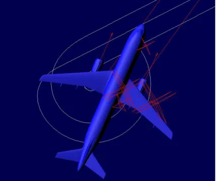
The manoeuvre chosen is the U-Turn (figure 1.1) which is the most demanding manoeuvre for aircrafts during ground operations. This manoeuvre induces the highest load on fuselage compared to the other ground manoeuvres; it is often performed using steering along with other systems such as differential braking and asymmetric thrust.
Figure 1.1 - U Turn manoeuvre
Key parameters used to evaluate the benefit of using flexibility in ground manoeuvrability modelling are:
1. Turning Radius 2. Turn Width 3. Tyre Side Forces
4. Torque between the main fitting and the strut 5. Computational time
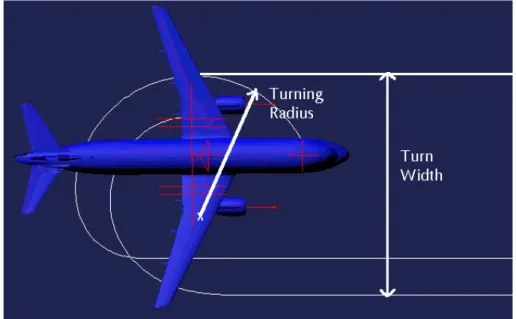
The first two parameters are the most interesting from a performance point of view because the aircraft has to meet the requirements for ground operations. The Turning Radius is the minimum radius of turning of the Nose Landing Gear during the manoeuvre.
The Turn Width is the minimum width of the runway that the plane needs to perform a U-Turn. Figure 1.2 shows Turning Radius and Turn Width.
Figure 1.2 – How to measure Turning Radius and Turn Width
Loads are not a required result when ELYD perform a ground manoeuvrability analysis. However loads allow a deeper understanding of the problem, for this reason Tyres Side Forces and Torque are considered part of the key parameters. Moreover Tyre Side Forces and Torque are essential characteristics for the understanding of the loads distributions during a turning.
The last parameter considered is the computational time. Very often ELYD is required to provide results where different aircraft configurations are coupled with several types of manoeuvre at different speed. The number of run can be very high, therefore the time to complete each run is important.
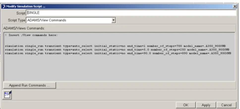
The simulations start with the aircraft suspended above the runway. At first it is dropped and let free to settle down for one second; then thrust and steering control are applied to perform the requested manoeuvre. The simulation does not start with the aircraft already on the ground because of solver convergence problems. Moreover it makes things easy in case of different investigations (e.g. different tyre dimensions or different oleo set up) because the model is ready to run since the tyres do not touch the runway.
In order to avoid errors and simulation failures, a higher number of steps is necessary during the first second of simulation in the rigid model (figure 1.3).
Figure 1.3 – Rigid model, simulation script
In the flexible models instead, in light of the higher number of parts and calculations, a higher number of steps is adopted during the first five second of simulation as shown in figure 1.4.
Figure 1.4 – Flexible models, simulation script
1.2 A350XWB Rigid-Flexible beam model comparison
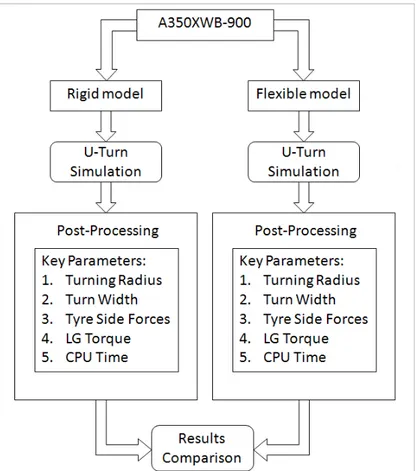
The first method for evaluating flexibility effects is done with a comparison between the A350XWB-900 Rigid model and the A350XWB-900 Beam
Flexible model. Figure 1.1 shows the process used to evaluate flexibility effects on ground manoeuvring simulations.
Figure 1.5 - Comparison between A350XWB-900 Rigid and Flexible models.
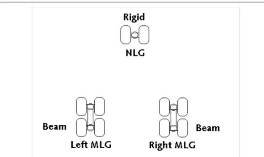
A Beam Nose Landing Gear was not available; hence the model is composed by a rigid Nose Landing Gear (NLG) and left and right beam Main Landing Gears (MLG) as shown in figure 1.6.
Figure 1.6 - A350XWB Flexible model setup
Using this model the following U-Turn cases have been investigated: 1. Symmetric thrust, no brake
2. Symmetric thrust, differential braking to initiate the turning
3. Symmetric thrust, differential braking hold during all the turning phase 4. Asymmetric thrust, no brake
5. Asymmetric thrust, differential braking to initiate the turning
6. Asymmetric thrust, differential braking hold during all the turning phase
For each case the following conditions apply: x Dry surface
x Speed 5 knots
x Max Steering Angle 75 deg
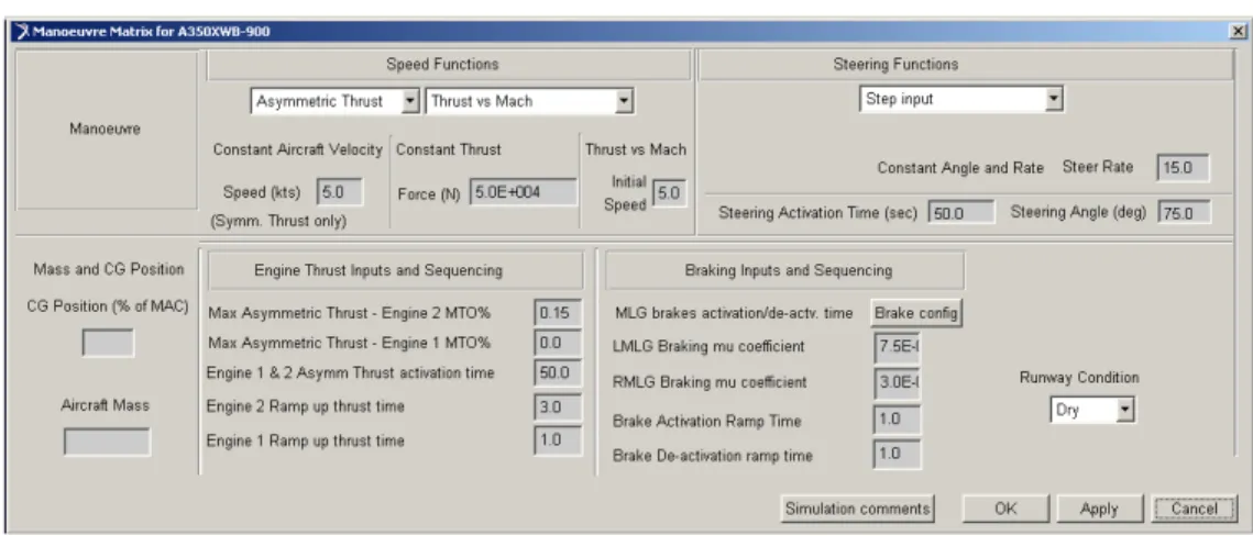
Figure 1.7 – Dialog box for selecting thrust, steering input
Using the dialog boxes shown in figures 1.7 and 1.8 it is possible to set different values of the design variables in order to simulate the requested scenarios.
Figure 1.8 – Dialog box for selecting brakes input
Turning Radius, Turn Width are computed as:
TURNING RADIUS: IF(WM(CG, Origin): VM(NLG_Axle_MARKER) /WM(CG, Origin), 0, VM(NLG_Axle_MARKER) /WM(CG, Origin)) 10
TURN WIDTH: IF(ABS(VARVAL(effective_NWS_SV)): 0,0, ((Wheel_Base_DV/1000)* (1+cos(DTOR*ABS(VARVAL(effective_NWS_SV))))/ (sin(DTOR*ABS(VARVAL(effective_NWS_SV)))) + (Track_Dimension_DV/2000 + 2.235/2 + 1.1425/2 ))) With: Effective NWS SV: JOINT_NWS_MEA - noseSlip_MEA 11
1.3 A320 Rigid-Flexible mnf comparison
Regarding the second approach to investigate the effects of flexibility, an initial work request was based on a model with both left and right flexible mnf Main Landing Gears and also a flexible mnf Nose Landing Gear.
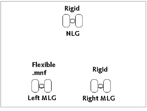
This time an A320 Landing Gear model was the only one available. Unfortunately only the flexible left Main Landing Gear has been provided, therefore the model has been setup as shown in figure 1.9.
Figure 1.9 – A320 Flexible model setup
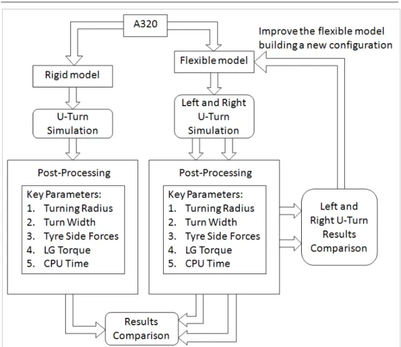
In this scenario and with this data available, a different comparison is necessary as shown in figure 1.10: left and right U-Turn have been investigated since the legs are not the same on the left hand side and on the right hand side. Results are not symmetric when changing turning direction; hence several configurations have been created introducing the flexibility in the right leg. These configurations allow understanding the trend of the ground manoeuvre performances and loads in function of the flexibility comparing the left and right U-turn.
13
Figure 1.10 – Comparison between A320 Rigid and Flexible models.
Once again the aircraft is dropped on the runway from a very short distance and let free to settle down for one second; then thrust and steering control are applied to perform the requested manoeuvre.
Due to the high number of models, only a symmetric thrust without braking U-Turn manoeuvre has been investigated; other conditions for the simulation are:
x Dry surface x Speed 5 knots x Symmetric Thrust x No brakes
x Max Steering Angle 70 deg
Turning Radius and the Turn Width are computed in ADAMS as follow:
TURNING RADIUS: IF(WZ(CG):
ABS(VM(NLG_Strut.NLG_Trail_Axle_Connect)/WZ(CG)), 0,
ABS(VM(NLG_Strut.NLG_Trail_Axle_Connect)/WZ(CG)))
LEFT TURN WIDTH:
ABS(DY(ground.TW_Wheel_4_MARKER, TW_NLGR_MARKER,
ground.TW_Wheel_4_MARKER))
RIGHT TURN WIDTH
ABS(DY(ground.TW_Wheel_1_MARKER, TW_NLGL_MARKER,
ground.TW_Wheel_1_MARKER))
The model displays automatically the correspondent Turn Width in the post processor, it depends if left or right turn has been selected
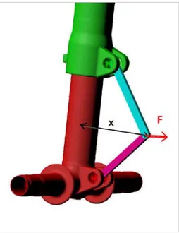
The Torque is computed directly when torsion spring is present. Otherwise when there is a rigid torque link the torque is computed as ܶ ൌ ܨݔ ; with F that is equal to the force in the lateral direction at the apex of the torque link and x is equal to the distance between the landing gear axis and the apex of the torque link as shown in figure 1.11.
Figure 1.11 – Flexible .mnf model Torque calculation