Chapter 4 – CODES AND PLANT MODELLING
4.1.
INTRODUCTION
In order to more accurately predict transient response, different combined 3D neutronic and thermal-hydraulic nodalizations were implemented for each reference case studied and depending on the coupled codes applied to it.
In the present work, two different coupled codes were used to model the plant in order to simulate a control rod ejection accident:
• RELAP 5/3.3-PARCS – this coupling requires external PVM to be operated.
• RELAP 5/3D-NESTLE – in this case the neutronic code is embedded in the TH code.
A brief description of these codes will be presented in the following section.
4.2.
ADOPTED COMPUTATIONAL CODES
4.2.1. RELAP5/ MOD 3.3
The RELAP5 computer code is a LWR transient analysis code developed mainly by the Idaho National Engineering Laboratory (INEL) for the U.S. Nuclear Regulatory Commission (NRC) for use in rulemaking, licensing audit calculations, evaluation of operator guidelines, and as a basis for a nuclear plant analyzer. Specific applications have included simulations of transients in LWR systems such as loss of coolant, anticipated transients without scram (ATWS), and operational transients such as loss of feed water, loss of offsite power, station blackout, and turbine trip.
The development of the code began at about 1970 and continues at our present time. The version used in calculations for this thesis was the RELAP5-MOD3.3 [12].
The code is based on a non-homogeneous and non-equilibrium model for the two-phases that is solved by a fast, partially implicit numerical scheme to permit economical calculation of system transients. The objective of the RELAP5 development from the outset was to produce a code that included important first-order effects necessary for accurate prediction of system transients but that was sufficiently simple and cost effective so that parametric or sensitivity studies were possible.
The code includes many generic component models from which general systems can be simulated. The component models include pumps, valves, pipes, heat releasing or absorbing
structures, reactor point kinetics, electric heaters, jet pumps, turbines, separators, accumulators, and control system components. In addition, special process models are included for effects such as form loss, flow at an abrupt area change, branching, choked flow, boron tracking, and non-condensable gas transport.
The system mathematical models are coupled into an efficient code structure. The code includes extensive input checking capability to help the user discover input errors and inconsistencies. Also included are free-format input, restart, re-nodalization, and variable output edit features. These user conveniences were developed in recognition that generally the major cost associated with the use of a system transient code is in the engineering labour and time involved in accumulating system data and developing system models, while the computer cost associated with generation of the final result is usually small.
Material properties are embedded into the code, but can also be supplied by the user. The numerical solution method has been specifically adapted for the code and is based upon the use of semi-implicit finite-difference technique. The thermal-hydraulic model can be classified as a ‘porous media’ type, to distinguish it from the ‘open media’ that is typical of Computational Fluid Dynamics (CFD) models. The code is capable of modelling the primary and secondary circuits of NPP as well as all the components belonging to the rest of the plant, including the related actuation logic.
The code is classified as a one-dimensional (1D) code, although ‘fictitious’ 3D nodalizations can be set-up to simulate three-dimensional flow configurations in open zones. For instance, the core of a NPP can be simulated by several (actually up to a few hundreds) parallel nodes interconnected at different axial elevations by ‘cross-junctions’.
4.2.2. PARCS
PARCS is a 3D neutron kinetics code developed for the NRC by the Purdue University [11]. The version used for the calculations in this thesis was one of the latest released at the present time (PARCS version 2.4.3).
PARCS is a three-dimensional (3D) reactor core simulator which solves the steady-state and time-dependent neutron diffusion equations to predict the eigenvalue and the dynamic response of the reactor to reactivity perturbations such as control rod movements or changes in the temperature/fluid conditions in the reactor core. The code is applicable to both PWR and BWR cores loaded with either rectangular or hexagonal fuel assemblies.
The neutron diffusion equation is solved with two energy groups for the rectangular geometry option, whereas any number of energy groups can be used for the hexagonal geometry option. PARCS
is coupled directly to the thermal-hydraulics systems codes TRAC-M and RELAP which provide the temperature and flow field information to PARCS during the transient. The thermal-hydraulic solution is incorporated into PARCS as a feedback into the few group cross-sections. The coarse mesh finite difference (CMFD) formulation is employed in PARCS to solve for the neutron fluxes in the homogenized nodes. In rectangular geometry, the analytic nodal method (ANM) is used to solve the two-node problems for accurate resolution of coupling between nodes in the core, whereas the triangle-based polynomial expansion nodal (TPEN) method is used for the same purpose in hexagonal geometry.
The major calculation features in PARCS include the ability to perform eigenvalue calculations, transient (kinetics) calculations, Xenon transient calculations, decay heat calculations, pin power calculations, and adjoint calculations.
The primary use of PARCS involves a 3D calculation model for the realistic representation of the physical reactor. However, various one-dimensional (1D) modelling features are available in PARCS to support faster simulations for a group of transients in which the dominant variation of the flux is in the axial direction, as for example in several BWR applications.
Numerous sophisticated spatial kinetics calculation methods have been incorporated into PARCS in order to accomplish the various tasks with high accuracy and efficiency. For example, the CMFD formulation provides a means of performing a fast transient calculation by avoiding expensive nodal calculations at times in the transient when there is no strong variation in the neutron flux spatial distribution. Specifically, a conditional update scheme is employed in PARCS so that the higher order nodal update is performed only when there are substantial changes in the core condition to require such an update. The temporal discretization is performed using the theta method with an exponential transformation of the group fluxes. A transient fixed source problem is formed and solved at each time step in the transient. For spatial discretization, the stabilized ANM two-node kernel or the multigroup TPEN kernel is used to obtain the nodal coupling relation that represents the interface current as a linear combination of the node average fluxes of the two nodes contacting the interface.
The solution of the CMFD linear system is obtained using a Krylov subspace method which utilizes a BILU3D preconditioner in rectangular geometry and a point ILU preconditioner in hexagonal geometry. The eigenvalue calculation to establish the initial steady-state is performed using the Wielandt eigenvalue shift method. The pin power calculation method employs a reconstruction scheme in which predefined heterogeneous power form functions are combined with a homogeneous intranodal flux distribution. The homogeneous flux shape is obtained by solving analytically a two-dimensional boundary fixed source problem consisting of the surface average currents specified at the four boundaries.
One of the essential neutronics problems for a reactor core is to represent the physical system with an accurate numerical model. Among the various fundamental modelling issues in the reactor kinetics calculation are the geometric representation, the cross-section representation, and the TH feedback modelling. PARCS provides a 3D geometric representation of the core that can be reduced to 2D, 1D, or 0D by the choice of the appropriate boundary conditions. However, a special 1D kinetics capability is also available for more accurate and versatile modelling.
PARCS can operate either with an internal limited TH model or coupled with other codes (TRAC or RELAP) that provide the TH model (external TH ). The time step size used in the system TH calculation is often selected very small because of numerical stability considerations. Sometimes it is so small that no considerable changes occur in the core TH condition and performing a neutronic calculation with such a small change would be unnecessary since the flux variation would also be small. For this, in order to improve code efficiency, a skip factor can be used in the coupled calculation such that the T/H code calls PARCS based on this user defined frequency.
PARCS uses macroscopic cross-sections which can be input in either the two-group or multi-group form using the same input cards. The macroscopic nodal cross-sections are functionalized on boron concentration (B, in ppm), square root of fuel temperature, moderator temperature and densities, void fraction and the effective rodded fractions. Only the linear dependence of cross-sections is considered on these state variables except for the moderator density and void fractions for which the quadratic variation is provided. Symbolically, the cross sections are functionalized as:
Here the effective rodded fraction is defined as the product of the volumetric rodded fraction and the flux depression factor that is computed by the decusping routine for the partially rodded node. For Xenon calculations, the Xenon and Samarium microscopic cross-sections are represented in the same form.
4.2.3. RELAP5/3D
RELAP5-3D, the latest in the series of RELAP5 codes, is a highly generic code that, in addition to calculating the behaviour of a reactor coolant system during a transient, can be used for simulation of a wide variety of hydraulic and thermal transients in both nuclear and non-nuclear systems involving mixtures of vapour, liquid, non condensable gases, and non volatile solute [27].
The mission of the RELAP5-3D development program was to develop a code version suitable for the analysis of all transients and postulated accidents in LWR systems, including both large- and small-break loss-of-coolant accidents (LOCA) as well as the full range of operational transients.
The RELAP5-3D version contains several important enhancements over previous versions of the code. The most prominent attribute that distinguishes the RELAP5-3D code from the previous versions is the fully integrated, multi-dimensional TH and NK modelling capability. This removes any restrictions on the applicability of the code to the full range of postulated reactor accidents.
Enhancements include a new matrix solver for 3D problems, new thermodynamic properties for water, and improved time advancement for greater robustness. The multi-dimensional component in RELAP5-3D was developed to allow the user to more accurately model the multi-dimensional flow behaviour that can be exhibited in any component or region of a LWR system. Typically, this will be the lower plenum, core, upper plenum and downcomer regions of an LWR. However, the model is general, and is not restricted to use in the reactor vessel. The component defines a one, two, or three- dimensional array of volumes and the internal junctions connecting them. The geometry can be either Cartesian (x, y, z) or cylindrical (r, θ, z). An orthogonal, three-dimensional grid is defined by mesh interval input data in each of the three coordinate directions.
The multi-dimensional neutron kinetics model in RELAP5-3D is based on the NESTLE code, briefly described in the next section.
4.2.4. NESTLE
There are two options for the computation of the reactor power in the RELAP5-3D code. The first option is the point reactor kinetics model that was implemented in previous versions of RELAP5. The second option is a multi-dimensional neutron kinetics model based on the NESTLE [13] code developed at North Carolina State University.
This option computes the reactor fission power in either Cartesian or hexagonal geometry. The nodal expansion method (NEM) is used to solve the neutron diffusion equations for the neutron flux in either two or four neutron energy groups. A flexible neutron cross section model and a control rod model have been implemented to allow for the complete modelling of the reactor core. The decay heat model developed as part of the point reactor kinetics model has been modified to compute the decay power for both the point reactor kinetics model and for the multi-dimensional neutron kinetics model.
The multi-dimensional neutron kinetics model in the RELAP5-3D code was developed to allow the user to model reactor transients where the spatial distribution of the neutron flux changes with time. The model solves the few-group neutron diffusion equation utilizing the Nodal Expansion
Method (NEM). It can solve the steady-state eigenvalue (criticality) and/or eigenvalue initiated transient problems. The subroutines used to solve the steady-state eigenvalue and the eigenvalue initiated transient problems were taken from the NESTLE code source, were modified to be compatible with the coding standards and data storage methodology used in RELAP5-3D.
RELAP5-3D was modified to call the appropriate NESTLE subroutines depending upon the options chosen by the user. The neutron kinetics model in NESTLE and RELAP5-3D uses the few-group neutron diffusion equations. Two or four energy few-groups can be utilized, with all few-groups being thermal groups (i.e. upscatter exits) if desired. Core geometries modelled include Cartesian and hexagonal. Three, two and one dimensional models can be utilized. Various core symmetry options are available, including quarter, half and full core for Cartesian geometry and one-sixth, one-third and full core for hexagonal geometry. Zero flux, non-reentrant current, reflective and cyclic boundary conditions are treated.
The few-group neutron diffusion equations are spatially discretized utilizing the Nodal Expansion Method (NEM). Quartic or quadratic polynomial expansions for the transverse integrated fluxes are employed for Cartesian or hexagonal geometries, respectively. Transverse leakage terms are represented by a quadratic polynomial or constant for Cartesian or hexagonal geometry, respectively. Discontinuity Factors (DF) are utilized to correct for homogenization errors. Transient problems utilize a user specified number of delayed neutron precursor groups. Time discretization is done in a fully implicit manner utilizing a first-order difference operator for the diffusion equation. The precursor equations are analytically solved assuming the fission rate behaves linearly over a time-step.
Independent of problem type, an outer-inner iterative strategy is employed to solve the resulting matrix system. Outer iterations can employ Chebyshev acceleration and the Fixed Source Scaling Technique to accelerate convergence. Inner iterations employ either colour line or point SOR iteration schemes, dependent upon problem geometry. Values of the energy group dependent optimum relaxation parameter and the number of inner iterations per outer iteration to achieve a specified relative error reduction are determined a priori. In addition, by electing to not update the coupling coefficients in the nonlinear iterative strategy, the Finite Difference Method (FDM) representation of the few-group neutron diffusion equation is used. The implication is that the model can be utilized to solve either the nodal or FDM representation of the few-group neutron diffusion equation.
The neutron kinetics subroutines require as input the neutron cross sections in the computational nodes of the kinetics mesh. A neutron cross section model has been implemented that allows the neutron cross sections to be parameterized as functions of RELAP5-3D heat structure
temperatures, fluid void fraction or fluid density, poison concentration, and fluid temperatures. A flexible coupling scheme between the neutron kinetics mesh and the thermal hydraulics mesh has been developed to minimize the input data needed to specify the neutron cross sections in terms of RELAP5-3D thermal hydraulic variables. A control rod model has been implemented so that the effect of the initial position and subsequent movement of the control rods during transients may be taken into account in the computation of the neutron cross sections. The control system has been modified to allow the movement of control rods by control variables.
The inputs to the kinetics modules in RELAP5-3D consist of neutron cross sections, boundary conditions, control flags, control data, etc. Neutron cross sections are needed for each neutron energy group and kinetics node and consist of the diffusion coefficient (D), absorption cross section (Σa), fission cross section (Σf), the product of the mean number of secondary neutrons per fission and the fission cross section (νΣf), and the scattering cross section for scattering into the neutron energy group from the other neutron energy groups (Σsg‘g). Discontinuity factors for each face of the kinetics nodes are also needed for each energy group. The user supplies the control information and the boundary conditions as part of the required input data. The neutron cross sections are computed from a function selected from a set of built-in functions or a user supplied function whose independent variables are weighted averages of RELAP5-3D hydraulic or heat structure variables. There are four built-in neutron cross section functions from which the user can select or the user may supply his own function in the form of an external subroutine.
A control rod model is used to determine the positions of the control rods and to compute the control rod variable needed by the neutron cross section function on each axial level in the reactor core. The three neutron cross section functions that the user may select to compute the neutron cross sections and the control rod model are described in the following section.
The first built-in cross section model is the RAMONA model. The RAMONA neutron cross section model uses the neutron cross section parameterization from the RAMONA-3B7.2-16 code. The functional form for the computation of cross sections is presented below:
The last built-in cross section model is the most general built-in cross section model and was developed as part of the RELAP5-3D code development project. The GEN cross section function uses a form similar to the HWR formulation except that the variable portion of the cross section is defined for three control states, active controlled, driver controlled and uncontrolled states. The GEN cross section function is given by :
The variations for the active controlled, driver controlled, and uncontrolled states are given by the equation above, where the coefficients a, b, c, d, and e are input separately for the active controlled, driver controlled, and uncontrolled states.
4.3.
COUPLING PROCESSES USED
4.3.1. RELAP/PARCS
The coupled RELAP5/PARCS codes use a General Interface, which manages the mapping of property data and solution variables between thermal-hydraulics and spatial kinetics codes. In this design, RELAP5, the General Interface, and PARCS are executed as separate processes and communicate with each other through the use of message-passing protocols in the Parallel Virtual Machine (PVM) package [14].
The coupled RELAP5/PARCS codes utilize an internal integration scheme in which the solution of the system and core thermal-hydraulics is obtained by RELAP5 and only the spatial kinetics solution is obtained by PARCS. In this scheme, PARCS utilizes the thermal-hydraulics solution data (e.g. moderator temperatures/densities and fuel temperatures) calculated by RELAP5 to incorporate appropriate feedback effects into the cross-sections. Likewise, RELAP5 takes the space-dependent powers calculated in PARCS and solves for the heat conduction in the core heat structures. The temporal coupling of RELAP5 and PARCS is explicit in nature, and the two codes are locked into the same time step. For this implementation, the RELAP5 solution lags the PARCS solution by one time step. Specifically, the advancement of the time step begins with RELAP5 obtaining the solution to the hydrodynamic field equations using the power from the previous time step. The property data obtained from this solution is then sent to PARCS and the power at the current time step is computed.
The two processes are loaded in parallel and the PARCS process transfers the nodal power data to the TH process. The TH process then sends back the temperature (fuel and coolant) and density data back to the PARCS process.
The user must run two programs simultaneously; the following sequence can be used during RELAP/PARCS coupling:
• run RELAP in the stand-alone mode for flow initialization (invoking no PARCS calculations) and generate a restart file at the end of the run (RELAP steady-state stand alone).
• using the above restart file, launch PVM and run the coupled steady-state case and generate the steady-state restart files for both PARCS and RELAP. Adjust the external TH skip factor so that excessive calls of PARCS are avoided. (RELAP/PARCS coupled steady-state).
In general, the neutronic node structure is different from the T/H node structure. The difference is reconciled by a mapping scheme. The original mapping was explicit in that the fractions of different TH nodes belonging to a neutronic node had to be specified in a file called MAPTAB for all the neutronic nodes. In order to reduce the user effort to prepare the MAPTAB file, automatic mapping schemes were developed for the coupled TRAC-M/PARCS code that take data from both PARCS and TRAC-M input files to generate the mapping information internally. Nevertheless, in the coupling process used in this work – RELAP 5/3.3-PARCS – the generation of the file MAPTAB was necessary. Automatic compilation of this mapping file was realized by the implementation of FORTRAN programs [29].
The MAPTAB file basically allows the association among thermal-hydraulic and neutronic nodes and through its functions it is possible to set the quantity of bypass associated to each node, the method of calculating Doppler temperature and the trip logics (e.g. to activate reactor scram).
4.3.2. RELAP 5/3D – NESTLE
As the code NESTLE is embedded in the RELAP5/3D program, no parallel code processing is required. On the other hand, all neutronic data must be inserted in the RELAP5/3D input deck, in a specific card for reactor kinetics.
The association between thermal-hydraulic and neutronic nodes is also inserted in this card, in a similar format as the MAPTAB file, the one used for the RELAP5/PARCS coupling.
Therefore, the user needs only to run RELAP5/3D in order to start simulation, instead of following the procedures explained in the previous topic, for the RELAP5/PARCS coupling. It seems also a way of reducing error in the process, as it is common (and it was experienced during the preparation of this thesis) to have errors during PVM operation while coupling process is being performed.
4.4.
THERMAL-HYDRAULIC MODELLING
The nodalization used for transient calculation was a modification of the previous one developed by the University of Pisa for the TMI-1 MSLB benchmark [6].
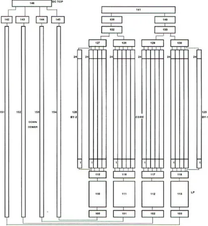
The sketch of the nodalization is showed in the Figure 4.2. It models the whole primary side (RPV, Hot Legs (2), Cold Legs (4), OTSG (2), Main Circulation Pumps (4) and ECCS) and the secondary side of the plant until the turbine. The nodalization was qualified as far as possible at the University of Pisa.
The main assumptions or relevant information for transient calculations are as follows:
• Assembly relative power distribution is given with quarter symmetry (as presented in Table 3.7);
• Axial power is assigned in 24 slabs not uniformly spaced; • The four MCP are assumed not to trip during transient;
• No credit is given to the operation of the pressurizer heaters and to CVCS;
• Boron concentration is assumed constant (5 ppm) and its reactivity is included in the overall moderator coefficient.
The main modifications of the core nodalization are here briefly summarized :
• addition of channel S (pipe 179), where rod ejection is supposed to occur, connected to branches branches 115 (LP) and 127 (UP), as can be seen in Fig. 4.3;
• creation of heat structure 1227 in the core, related to the FA where rod ejection is supposed to occur;
• new assignment of the mass flow, flow area, etc. for modified core channels;
• new assignment of the heat exchange surfaces, relative power coefficients, etc. for modified core structures;
• generation of spatial mapping file (MAPTAB) for NK-TH nodes association;
• new assignment of neutronic parameters in NK input deck for PARCS and RELAP5/3D; and • creation of new TH and NK input decks for HZP and HFP for all reference cases studied and
For the purpose of obtaining BE results, an increase of the details of the core nodalization was needed. Therefore, a new nodalization of the part of the core interested by the rod ejection was developed, by the insertion of a single thermal-hydraulic channel (Channel S) corresponding to the FA where a REA was postulated.
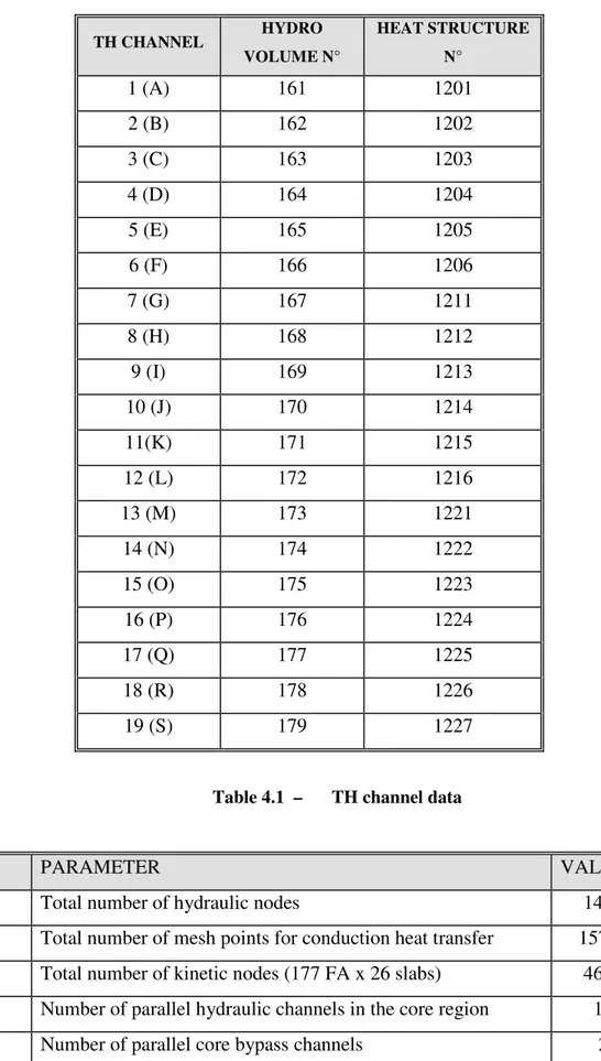
The final nodalization described the core through 21 independent thermal-hydraulic channels, 19 describing the FA channels (Table 4.1) and 2 describing the core by-pass (Vol. 125 and 126) as indicated in Fig. 4.2 and 4.3. Limitations in the maximum number of junctions belonging to a single branch (RELAP 5 component) imposed the need to split the lower and upper plena in four parts, at least in the zones of connection between the LP and the UP with the core itself. The downcomer has been split in four parts, corresponding to the four Cold Legs of the plant. The coolant flowing in one part does not mix with the others. The UP has been divided in two parts, corresponding to the number of Hot Legs. A detailed nodalisation of the core region is then presented in Fig. 4.2 and 4.3.
The dimension of the nodalization can be observed from the data presented in Table 4.2:
115
116
117
118
127
128
129
130
126 125A G M N
S
A G M N
A G M N
S
B C H I O
B C H I
B C H I O
P J D E K
P J D E
P J D E K
A G M N S
A G M N
A G M N S
P J D E K
P J D E
P J D E K
A G M N S
A G M N
A G M N S
B C H I O
B C H I
B C H I O
A G M N
S
A G M N
A G M N
S
Figure 4.3 – Detailed nodalization of core channels, indicating channel S
1 2 3 4 5 6 7 8 9 10 11 12 13 14 15 16 17 1 2 14 14 14 14 14 3 15 14 14 14 14 14 14 14 13 4 15 15 9 8 8 8 8 8 7 13 13 5 15 15 15 9 8 8 8 8 8 7 19 13 13 6 15 9 9 9 3 2 2 2 1 7 7 7 13 7 15 15 9 9 3 3 2 2 2 1 1 7 7 13 13 8 15 15 9 9 3 3 3 2 1 1 1 7 7 13 13 9 16 15 9 10 4 3 4 2 6 1 6 12 7 13 18 10 16 16 10 10 4 4 4 5 6 6 6 12 12 18 18 11 16 16 10 10 4 4 5 5 5 6 6 12 12 18 18 12 16 10 10 10 4 5 5 5 6 12 12 12 18 13 16 16 16 10 11 11 11 11 11 12 18 18 18 14 16 16 10 11 11 11 11 11 12 18 18 15 16 17 17 17 17 17 17 17 18 16 17 17 17 17 17 17
TH CHANNEL HYDRO VOLUME N° HEAT STRUCTURE N° 1 (A) 161 1201 2 (B) 162 1202 3 (C) 163 1203 4 (D) 164 1204 5 (E) 165 1205 6 (F) 166 1206 7 (G) 167 1211 8 (H) 168 1212 9 (I) 169 1213 10 (J) 170 1214 11(K) 171 1215 12 (L) 172 1216 13 (M) 173 1221 14 (N) 174 1222 15 (O) 175 1223 16 (P) 176 1224 17 (Q) 177 1225 18 (R) 178 1226 19 (S) 179 1227
Table 4.1 – TH channel data
N° PARAMETER VALUE
1 Total number of hydraulic nodes 1499
2 Total number of mesh points for conduction heat transfer 15700 3 Total number of kinetic nodes (177 FA x 26 slabs) 4602 4 Number of parallel hydraulic channels in the core region 19
5 Number of parallel core bypass channels 2
6 Number of elements in each core stack 26
4.5.
3D NEUTRON KINETIC MODELLING
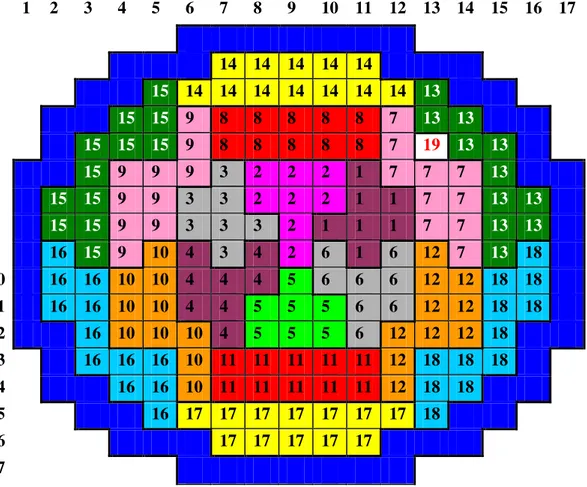
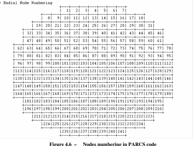
The reactor core was divided in two regions: active core and the reflector region, as indicated in Fig. 4.6, corresponding to the PARCS nodalization. The model consists in 241 assemblies, among these 177 fuel assemblies and 64 reflector assemblies. Sixty-one of the 177 FA were considered ‘rodded’ FA, in order to model their capacity of hosting a CR cluster.
Figure 4.5 – PARCS output of radial core representation
Relevant data about the NK nodalization was already presented in Chapter 3, when a detailed description of the core was given.
Thirty types of assembly were used to describe the different physical composition of the core (see Table 3.11). Axially, the active core is divided in 24 layers with varying heights, adding up to a total core height of 357.12 cm. In addition, both the upper and lower axial reflectors have a thickness of 21.811 cm. The energy release per fission for the two prompt neutron groups was fixed at 0.3213 x10⁻¹⁰and 0.3206 x10⁻¹⁰J/fission.
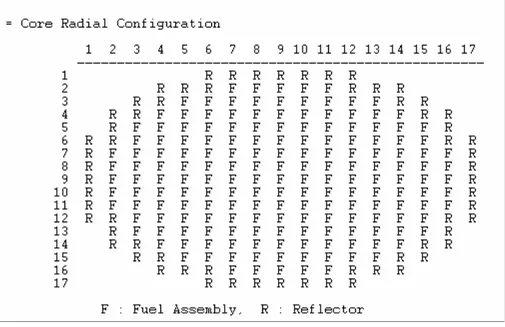
A tough task connected to the NK nodalization is related to the study of the NK codes adopted, in order to comprehend the methodology and parameterization used to model the reactor core in 3D. As an example, Fig. 4.6 presents how the PARCS code numbering is implemented, as this is an important parameter for spatial mapping generation (MAPTAB file). Nestle code, on the contrary, uses thermal-hydraulic zones mapping to do this, as a part of the NK input deck, and node numbering in this case is not a relevant parameter.
Figure 4.6 – Nodes numbering in PARCS code
Understanding the way codes model control rod data was also fundamental in order to enable simulation of the ejection of a CR. An example of control rod modelling is presented in Fig. 4.7.
In the development of the present work, PARCS input file served as the basis for deriving RELAP 3D neutronic data. For example, in order to prepare cross section data in the table format required by RELAP 3D, there has been the need of developing FORTRAN programs.
A complete set of diffusion coefficients and macroscopic cross-sections for scattering, absorption, and fission as a function of the moderator density and fuel temperature is defined for each composition. The assembly discontinuity factors (ADFs) are taken into consideration implicitly by incorporating them into the cross-sections in order to minimise the size of the cross-section tables.
4.6.
CONTROL ROD WORTH CALCULATION
In order to identify the control rod assembly whose ejection from the core causes the highest insertion of reactivity, the neutronic code PARCS was performed in a stand-alone mode.
Two states of the plant were analyzed in this procedure: the Hot Full Power (HFP) and the Hot Zero Power (HZP), to provide calculation in two different power conditions. The first state implies a transient to a fuel that is at high temperature as long as the second state could lead to a severe transient for the clad because minor coolant flow is associated with fewer pump in operation.
The HZP and HFP with the nuclear fuel at EOC were analyzed, assuming β = 5.2 x 10⁻³. The control rod was always assumed to be ejected in 0.1 seconds from the fully inserted to the completely withdrawn position, in the HZP case. In the HFP condition, at EOC, all the control rod banks are supposed to be withdrawn from the reactor core; therefore a CA ejection was idealized from a 40% to 100% extracted position.
The scram delay signal was assumed to be 0.3 seconds and the time for the complete insertion of all the CA was assumed to be 2.3 seconds. In table 5.2 the main parameters imposed for the definition of the plant status are summarized.
Calculation was performed through a series of steady-state calculations of the keffective (k1) assuming the CR banks positions described in Fig. 4.8 and the control rod that has to be ejected in its initial position. Then it was performed a steady-state calculation of the keffective (k2) with this control rod completely withdrawn. The reactivity insertion was therefore calculated by the formula :
This procedure was first used to identify the rod bank with the highest value of rod worth; after this, among the rods belonging to this bank, the most reactive control assembly was identified.
1 6 1 3 5 5 3 7 7 7 3 5 4 4 5 3 1 6 2 6 1 5 4 2 2 4 5 6 7 2 7 2 7 6 5 4 2 2 4 5 1 6 2 6 1 3 5 4 4 5 3 7 7 7 3 5 5 3 1 6 1
Figure 4.8 – Control rod banks in the core
HOT ZERO POWER HOT FULL POWER
Core Power 0.1% PN 100% PN
PRZ pressure (MPa) 14.96 14.96
Boron Concentration (ppm) 5.0 (EOC) 5.0 (EOC)
Core inlet coolant temperature (°K) 551 551
Fuel Average Temperature (°K) 551 921
CR bank position I to VII A.R.I * I to VII A.R.O.*
Transient 1 CR ejected in 0.1 s
Scram set point: 114 % PN
1 CR ejected in 0.1 s Scram set point: 114% PN
Scram delay signal (s) 0.3
Scram time (s) 2.3
* A.R.O. → All rods out ; A.R.I → All rods in
Table 4.3 – Main plant parameters for HZP and HFP used in rod worth calculation CR to be ejected
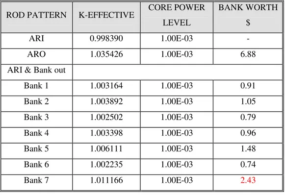
ROD PATTERN K-EFFECTIVE CORE POWER LEVEL BANK WORTH $ ARI 0.998390 1.00E-03 - ARO 1.035426 1.00E-03 6.88
ARI & Bank out
Bank 1 1.003164 1.00E-03 0.91 Bank 2 1.003892 1.00E-03 1.05 Bank 3 1.002502 1.00E-03 0.79 Bank 4 1.003398 1.00E-03 0.96 Bank 5 1.006111 1.00E-03 1.48 Bank 6 1.002235 1.00E-03 0.74 Bank 7 1.011166 1.00E-03 2.43
Table 4.4 – Bank worth for HZP
ROD PATTERN K-EFFECTIVE CORE POWER
LEVEL
BANK WORTH $
ARI 0.97515 1.00E+00 -
ARO 1.014004 1.00E+00 7.17
ARO & Bank in
Bank 1 1.010584 1.00E+00 0.64 Bank 2 1.010638 1.00E+00 0.63 Bank 3 1.010693 1.00E+00 0.62 Bank 4 1.009912 1.00E+00 0.77 Bank 5 1.007438 1.00E+00 1.23 Bank 6 1.010688 1.00E+00 0.62 Bank 7 1.003103 1.00E+00 2.06
As can be seen in the previous tables, the CR Bank n° 7 possesses the highest rod worth for both HZP and HFP conditions. After further calculation, among those rods belonging to Bank n° 7, the CA in the position (13,5), as indicated in Fig. 4.8, was identified as the CR having the highest worth in the core.
Thus, for every transient performed later in this work, it was assumed a REA caused by this CR failure, that will be named after CA n° 8, as indicated in Fig. 4.9, corresponding to the nodalization used in PARCS calculations.
Table 4.6 presents, for each power condition analysed, the corresponding rod worth value for CA n° 8, obtained through steady-state calculation performed with the PARCS code.
Figure 4.9 – PARCS nodalization for control rod bank configuration, indicating rod to be ejected during accident simulation
POWER CONDITION CORE POWER LEVEL CA#8 WORTH $ HZP 1.00E-03 0.74 HFP 1.00E+00 0.19