3
Chapter 2
THE HANDLING DIAGRAM THEORY
2.1. Introduction
The handling diagram is one of the most important tools of the vehicle dynamic and was presented by H. B. Pacejka in [4]. It consists of a curve that provides the whole steady-state cornering conditions of a vehicle and defines its directional behavior.
This diagram is also useful to define the understeering gradient K of the vehicle, which is the slope of the curve; furthermore, it allows drawing some conclusion about the stability of the vehicle. Because of all these reasons, it is possible to extract from it different information and evaluate the performance of a vehicle. It is worth remembering that such diagram refers to vehicles fitted with an open differential. In this particular case, a “single handling diagram”, only depending upon the constructive parameters, is found. Indeed, it was shown by [5], [7] that the handling diagram becomes completely inadequate for vehicles fitted with locked differential; it becomes part of a more general problem that leads to the definition of a “handling surface”, to which the handling diagram is just a special case.
In the thesis only vehicles fitted with open differential will be taken in consideration, so that the classical approach of the handling diagram is sufficient. However, the handling diagram will be plotted as function of a parameter which is the tire inflation pressure. Thanks to this approach, it is possible to obtain different handling diagrams for the same vehicle, which constitutes a “handling surface”: the aim is to understand if such handling surface can be used and developed to visualize the influence of tyre pressure. This will be presented in details in the fifth chapter.
4
2.2. Vehicle model
2.2.1. Introduction
In order to understand the meaning of the handling diagram is necessary to introduce a single-track vehicle model. Its characteristics were deeply explored by many authors in literature [1], [2], [3]]. It’s important to understand the entire hypothesis there are behind this model: only after this it is possible to accept the single-track model as a valid scheme for vehicle. All the studies and results presented in this thesis are based on this model, which is here briefly presented.
2.2.2. Single-track vehicle model
Figure 2-1 - Single-track vehicle model
The single-track vehicle model refers to a rear-wheel drive vehicle fitted with an open differential. As shown in Figure 2-1, the vehicle model is represented as a rigid body fitted with two equivalent tires, which simulate the behavior of the front and rear axles. A plane motion parallel to the road is considered.
5
A not showed reference frame attached to the vehicle is defined; its origin coincides with the centre of mass and its unit vectors are . Axes i and j are parallel to the road. The direction of axis i coincides with the forward direction of the vehicle, while axis j is orthogonal to that direction and points to left side of the vehicle. Axis k is orthogonal to the road and points upwards.
The position of the center of mass is defined by the two quantities and (longitudinal distances between the center of mass and each axles); the wheelbase is given by . The speeds u and v are the longitudinal and lateral components of the absolute speed of the centre of mass (2.1), whereas r is the yaw rate and it is component of the vehicle angular velocity (2.2):
The quantity represents the front steer angle. R expresses the distance between
the instant centre of rotation C of the vehicle and its longitudinal axis (2.3):
One of the most important kinematics parameters is the vehicle attitude angle β,
defined as (2.4):
Front and rear slip angles are now introduced. They are connected to the previous kinematics quantities through the following relations (2.5),(2.6):
6
In the Figure 2-1 forces and are also shown. They represent lateral forces acting on front and rear equivalent tyres.
The acceleration of the centre of mass is (2.8):
where is the longitudinal acceleration and is the lateral acceleration.
For the steady state conditions of the vehicle it is useful to introduce the steady state lateral acceleration (2.9)
:
If the longitudinal speed u is supposed given, there are only two equations that govern the model dynamics, which are (2.10), (2.11):
where m is the vehicle mass and is the vehicle moment of inertia with respect to
the vertical axis k passing through the centre of mass . The are the constitutive equations of the tire, which represents the non-linear relationship between the lateral force and the slip angle of each axle.
7
2.3. Handling diagram and understeering
gradient
The steady-state equations of motion can be obtained by considering the equations (2.10),(2.11) and :
Once the steady state lateral acceleration is assigned, it is possible to solve the system given by (2.12), (2.13) to obtain the two quantities and . As a consequence, and are functions of , and also the difference is function of the same quantity.
It is easy to demonstrate that the previous difference is equal to the difference between the steering angle and the Ackermann angle , which, in a compact form is (2.14):
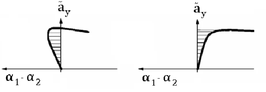
This function is the so called handling equation, which is one of the most useful tool for the analysis of the directional behavior of the vehicle. As an aid to explain such analysis, Pacejka created the handling diagram. This is a two-dimensional plot with the steady state lateral acceleration on the ordinate and the tire slip angle difference on the abscissa. The handling equation is plotted on this plane. In Figure 2-2 two different examples of such a handling diagram are presented (only positive
8
Figure 2-2 – Different examples of handling diagram
Note that the quantity is positive to the left. The shape of the handling diagram depends on constructive parameters of the vehicle and the axles characteristics.
The understeering gradient K is now introduced as follows (2.15):
It represents the slope of the handling curve in correspondence of a particular value of and provides a direct indication of the understeering-oversteering behavior of the vehicle:
if (positive slope) the vehicle is defined understeer if (vertical slope) the vehicle is defined neutral if (negative slope) the vehicle is defined oversteer
These definitions are valid for the single-track model presented and depend on the constructive characteristics of the vehicle considered. The understeering gradient is only function of the steady state lateral acceleration, so that the understeering-oversteering behavior of the vehicle is not affected by the steady-state maneuvers performed.