PERFORMANCE RESULTS
After having analysed in details the bitallocation algorithms and the new DSM technique in the previous chapters, we now investigate on DSM level-1 with simulation results coming from the use of the Dynamic Simulation Tool1.
Our aims:
• Quantize the gains of DSM level-1 with respect to the reference bitallocation for actual ADSL.
• Fully understand the behaviour for steady-state of the lines that apply DSM. Our characteristic approach:
• Simulations will be conducted using as input real data coming from the real fields. (For example no uniform distribution are used neither optimal testing topologies are created).
• No worst case scenario will be used, but we will work with a statistical approach.
• To obtain reliable results with this approach a good number of simulations has been done trying to obtain as much results as possible.
Our limits:
• As all the implemented tools, also our tool presents some approximations. They are mentioned in chapter 6 and we will recall in section 7.1.1 the assumptions important for our analysis.
1
• One could object that our study is too much related to the limits of statistical approaches. To restrict this limits, a deep study of the results has been done with a double purpose: avoid a sterile presentation of data and give a good interpretation of them in order to extrapolate general advices extendible to any network.
7.1 Simulation environment setup
To achieve the aims just mentioned, we have structured our analysis considering the variation and/or combination of the following parameters:
• Two of the three different deployment scenarios depicted in 5.3.2 are exploited: CO unbunched and CO/RT.
• Two different length distributions are used: European distribution and American distribution.
• Different noise sources and combinations are used: AWGN, SHDSL, HDSL, ISDN.
• To have a good comprehension on the gains and on the behaviour of the DSM lines, different percentage of lines that apply DSM are used.
• Since the operators offer to the user only some possible values for the bitrate, we have decided to use only a real set of Target Bit Rate for testing DSM gains.
We want to foresee in which deployment and noise scenario DSM can be beneficial.
One noteworthy point is our particular choice of inputs in the simulations: we have used real cable scenario information coming from statistical data and a set of target bitrates that are normally chosen today by operators.
This is a substantial difference from the simulations normally conducted up till now: no worst cases are used anymore, but the real scenarios are analyzed and no optimal conditions for the implementation of the algorithm are satisfied, but results on how the algorithm adapts itself to the real data are analysed.
Since DSM is “dynamic” in the meaning that it adapts to the conditions, this choice has seemed to us the best one for our purpose of giving a good view of DSM performance in the real actual networks. However, we will add detailed comments to all the results, in order not to give only sterile data presentation, but general advices extendible to any network.
7.1.1 Approximations
• Bitallcation follows the theoretic Shannon formula: bits are real and not integer, so gi=0. This allows to give the maximum data rate possible without limits of implementations for both actual bitallocation and DSM algorithms.
• Bitswap: Currently for each time in the simulation, the optimal bitloading is being calculated. If there is a difference from the previous bitloading then all tones are bit swapped in one message. This allows to give the maximum data rate possible without limits of implementations of the bitswap algorithm, but, at the same time, gives more instability to the lines that change instantaneously the bits on all tones (while in the real bitswap the process is longer and can give the time to the external changes to come back to the previous conditions without having changed too much the line conditions).
• Monitored tones: To obtain the best power allocation, we always monitor the SNR on all the tones, without allocating energy on the tones not used, while in reality, only some tones are used to monitor the SNR since on that tones the modems need to allocate a minimum amount of energy. (see 3.2)
• We only look to the steady-state performance and not to the stability. In reality it may be difficult to reach this steady-state performance in a stable way (without too many re-initializations). This is important because a modem that uses power back off, will still start up at maximum PSD, so at that time this line could destabilize other lines. This transition effect is not taken into account.
7.1.2 Fixed parameters and methods
Common to all the simulations
• Loop Type = ANSI 26 Awg. • PSD AWGN = -140 dBm/Hz.
• Flat PSD: is used thanks to the flat PSD discovery (see 4.2). • Tones used in Upstream band = [7:31].
• Tones used in Downstream band = [32:255]. • Shannon Gamma = 12 dB.
• Shannon Efficiency = 0.8 (it takes into account the efficiency of the actual bitloading respect to the shannon formula).
• Bitrate Overhead = 32000 bit/sec (it takes into account 1 byte per symbol due to the channel overhead).
• Minimum number of bits on each tone = 2. • Maximum number of bits on each tone = 14.
• Data symbol = 4000 symbol/sec (this value takes into account the tone spacing, the prefix cyclic, the sync symbols).
• TargetNoiseMargin = 6 dB (see 3.1.3). • MinimumNoiseMargin = 3 dB (see 3.1.3).
Reference parameter (without DSM)
• Dsm = ‘none’; it’s margin adaptive mode operation. • MaxAddNoiseMargin = infinitive.
• PSD = - 40 dBm/Hz.
DSM parameters
• Dsm = ‘flatboost’ (see 6.2.4); it’s DSM level-1 with boosting allowed. • MaxAddNoiseMargin = 0.
7.1.3 Parameter Combination
7.1.3.1 Scenarios
We test DSM in the CO unbunched scenario and in the CO/RT scenario.
The CO unbunched scenario is the common scenario in which ADSL is deployed nowadays: results coming from this scenario quantize the possible improvements derived by applying DSM level-1 in the actual modems.
The CO unbunched scenario used in our simulation is composed by 16 ADSL lines; for each simulation we have tested 30 topologies of 16 lines of random variable lengths coming from the European and American distributions.
For the CO/RT scenario, we have studied the improvements when applying DSM only at the RT lines: results coming from this scenario, on one hand show the effects of DSM used only as power Backoff and, on the other hand, quantize the possible gains derived by applying DSM in the new modems installed at the RT while not changing the old ones at the CO. We have to precise that this scenario is not yet realistic for ADSL: the RT starting from the last section is nowadays foreseen only for VDSL, but our results are an indication of how big could be the gain with this deployment.
The CO/RT scenario used in our simulation is composed by 16 ADSL lines in total: 8 lines at CO and 8 lines at RT; for each simulation we have tested 50 topologies of random variable lengths coming from the European and American distributions.
In this way the number of data points coming from the simulations when looking at the CO gains is of the same order of magnitude as the CO unbunched simulations and our comparisons between the two scenarios will be trustworthy.
With these tests, we have the complete basic cases of DSM level-1 applied by ADSL modems.
7.1.3.2 Length distributions
In order to give results as close as possible to the ones achievable in a real topology, we have tested the DSM level-1 technique using the real length distribution.
Two different length distributions are used: the European and the American one. These two cable plants differ sensibly: while the European distribution has a high percentage of short loops, the American one, on the contrary, presents a high number of long lines: testing these two curves we are able not only to give information on the behaviour of DSM level-1 in the real fields, but we can also extrapolate some general conclusions on DSM level-1 gains respect to short or long loops.
Next figure depicts the “American loop length distribution” and the “European loop length distribution” used in our simulations and depicted in a cumulative way:
Figure 7.1: Loop Length Distribution
Our topologies are generated with a random process (within the possible values coming from the distribution).
Since we are testing with a finite number of topologies and simulations, the distribution used in the simulations differs slightly from the theoretical one.
Next figure shows the differences between the “Theoretical distribution” and the “Simulated distribution” used to simulate the European configuration.
As we can see, differences are small; this validate the reliability of our results.
Figure 7.2: Theoretical and Simulated Distribution
7.1.3.3 Noises
Different noise sources and combinations are used.
AWGN, ISDN (DSL G9961), SHDSL and HDSL are the noise sources tested and the ETSI FB combination model have been simulated.
Next figure shows the PSD masks used:
Figure 7.3: PSD Noise Mask
When we speak of other technologies (HDSL,SHDSL,ISDN) together with ADSL, that is referred to be Spectral Management. Since DSM origins its name from the concept of Dynamic Spectral Management, we want to test how much DSM is influenced by the other technologies and which is the best noise environment.
Normally not all the lines in a binder are ADSL and the DSM level-1 gain will be influenced by all the other lines that don’t apply it.
Since we want to give advices for different noise combination, we have tested following the sequent procedure:
• First, only one noise at one time with different quantity (0 4 10 15) has been simulated, in order to give feedback on how DSM level-1 works against a certain single noise type.
• Secondly the ETSI FB noise combination ( 10 DSLs G9961, 4 HDSLs, 15 SHDSLs) has been tested, in order to give the gain for this combination and to extrapolate conclusions about prediction of combination of noises just knowing the behaviour of DSM level-1 against the single noise sources.
7.1.3.4 DSM Percentage
Different percentage of number of ADSL lines that apply DSM level-1 have been tested, in order to analyse if DSM can gain even if not all the lines use it.
DSM percentage = 20%, 50%, 100% has been tested, where the lines that apply DSM are randomly chosen without following any rule of optimality.
7.1.3.5 Set of target bitrate
As explained in 5.3.2, the algorithm can converge to a stable point only if the set of target bitrate is achievable. If the target bitrates belong to the rate region, than the Nash theorem assures the convergence of the algorithm to the minimum amount of power that each user has to set to achieve its own target bitrate.
Nowadays most of the operators work with a fix set of target bitrates: they can only provide certain values of target bitrates.
We have chosen to test DSM with the following realistic tuples of target bitrate: • [5.5 Mbit/sec, 3.5 Mbit/sec, 1.5 Mbit/sec, 256 kbit/sec]
• [5.5 Mbit/sec, 3.5 Mbit/sec, 1.5 Mbit/sec]
When initialising, each modem computes its maximum attainable bitrate and sets as target bitrate the maximum achievable bitrate within these values.
Using these realistic values, we can test the increase in rate/reach for real profiles, we can find the rate region within these values and we can test the convergence of the algorithm.
We have used these 2 tuples, that differ only for the presence/absence of 256 kbit/sec, because we want to quantify the effect of boosting (see 4.3.2) on very long lines.
While with the first tuple the very long lines will do a lot of boosting that can influence negatively the performance of short lines, with the second one the longer lines will not be able to activate themselves and we will test which increase is present for the short lines when they are the only ones to apply DSM.
7.2 Performance Results
In this section we show and comment the results obtained looking at the variation of one parameter each time, fixing the others under some assumptions.
The gains are quantified either with plot and either with percentage numbers.
7.2.1 Plot used
We will give information of the gains either referring to the loop length reached, either referring to the total coverage reached. To achieve it we use 3 different plots:
1. Service bitrate with respect to the coverage of the total network.
2. Data point plots with statistical average of Service bitrates with respect to loop length reached.
3. Plots of Service bitrate with respect to loop length with 99% certainty.
1. Service bitrate with respect to the coverage of the total network.
This plot depicts the cumulative percentage of the lines that can reach a certain bitrate respect to the total number of lines tested.
An example is given in the following figure, where saying that the 75% of the lines reach 1,5 Mbps means that the 75% of the lines can reach at least 1,5 Mbps; so the percentage of lines that can reach at least 256 kbps (the lowest service bitrate) indicates the percentage number of activated lines.
Figure 7.4: Service Bitrate with respect to Coverage
2. Data point plots with statistical average of Service bitrates with respect to loop length reached.
Since also the loop length distribution is given in a cumulative way, we can extrapolate loop reach information from the cumulative plot, using the distribution plot as a conversion factor. This information can be plotted together with the real data points coming from the simulations as in the following example, where the circles are the data points and the straight line indicates the average loop length found from the coverage.
Figure 7.5: Service bitrate with respect to statistical loop length
3. Plots of service bitrate respect to loop length reached with 99% certainty. This type of plot is more conservative: it identifies the loop length reached by the 99% of the lines with a certain service bitrate with respect to all the lines shorter than that length.
As we can see comparing the following figure with the previous one (they are made from the same data), the information that we get with the 99% certainty plot is quite similar to the statistical average if there are not too many lines of the same length that can have as a stable point within two different bitrates; on the contrary, if there are too many lines spread in a huge range of lengths that can have two different bitrates, the results coming from the two graphical approach are slightly different. For not making heavy our report, we have chosen to show the gains for loop length only with one method and to be sure that our indication about the length reached cannot give problem to the operators, we will plot only the 99% certainty. To obtain
the real gains of the statistical average length reached, one can always refers to the procedure explained in point 2.
Figure 7.6: Service bitrate with respect to loop length 99% certainty
7.2.2 DSM percentage
For the analysis of DSM percentage, we present only one plot that exemplifies the main aspects regard this topic; small differences are present depending on the loop length distribution and the type and number of noises, but those differences follow the behaviour that will be presented in the next paragraphs.
The general behaviour of DSM depending on the percentage of lines that apply it, is summarised in the following points:
• with a casual 20% of the ADSL lines that use DSM, the gain is very small. • with a casual 50% of the ADSL lines that use DSM, the gain is approximately
half the gain with full DSM.
Next figure plots the results for the European loop length distribution with 10 SHDSL noise sources .
Figure 7.7: DSM percentage analysis
We can conclude that DSM level-1 has, with respect to the reference ADSL, a gain that increases linearly with the number of lines that apply it; significant gains are present only when all the lines are able to use the DSM level-1 algorithm. The gains can justify the efforts spent for applying DSM level-1 to all the lines.
On the longest lines with the 256kbps profile, we can see a gain that is in proportion with the number of lines that apply DSM.
Due to that, next analysis will be conducted comparing the actual reference ADSL bitallocation only with respect to the DSM level-1 algorithm applied to all the ADSL lines.
7.2.3 Target Bitrate: Boosting effects
Comparing the rate region for the following tuples of data rate • [5.5 Mbit/sec, 3.5 Mbit/sec, 1.5 Mbit/sec, 256 kbit/sec] • [5.5 Mbit/sec, 3.5 Mbit/sec, 1.5 Mbit/sec],
we haven’t found significant increases in the number of short lines that can achieve a higher bitrate due to less crosstalk when the very long lines, that apply boosting, are not activated.
This means either that the long lines at 1.5 Mbit/sec already do lot of boosting or either that the effects of boosting is not so significant in loss of performances.
The average increase is 1 line more that sets its profiles from 3.5 Mbit/sec to 5.5 Mbit/sec: in percentage this increase is not so significant either for European and American distributions.
Moreover, no big differences are present between the increases in the European and in the American distributions: since the American distribution has more long lines, we expected better increases for these cases, because more long lines that do boosting are shut down. This result confirms that boosting of the very long lines doesn’t create too much loss on performance of short lines.
The following table summarises our results:
Scenario European gain of 3 profiles respect to 4 profiles.
American gain of 3 profiles respect to 4 profiles.
AWGN d 100 1 line 1 line DSL n 4 d 100 0 line 0 line HDSL n 4 d 100 0 line 2 line SHDSL n 4 d 100 0 line 0 line DSL n 10 d 100 1 line 1 line HDSL n 10 d 100 1 line 2 line SHDSL n 10 d 100 4 line 2 line DSL,HDSL,SHDSL n 15 d 100 1 line 1 line
The best increase we noticed, is for the European distribution with 10 noises, where there are 4 lines more that can achieve 5.5 Mbit/sec instead of 3.5 Mbit/sec, but there is also a loss in the total number of lines that can achieve at least 1.5 Mbit/sec.
So no advantages for DSM come out by disabling only the longest lines.
Next figure shows how small the increase is:
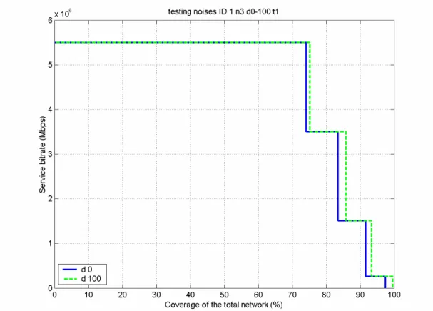
Figure 7.8: Boosting effects on very long lines
Summarising, the analysis presented lets us conclude that an operator, with DSM level-1, could choose to insert a low profile without loosing in performance: it will increase its base of customers at a long distance, simply offering a low profile at a low cost, while assuring the same performance to all the other customers.
DSM grants the privilege of variety in profiles.
From conclusions of paragraphs 7.2.2 and 7.2.3, next analysis will be conducted comparing the actual reference ADSL bitallocation with respect to the DSM level-1 algorithm applied to all the lines and with the highest number of profiles.
7.2.4 CO unbunched
The CO unbunched scenario is the common scenario in which ADSL is deployed nowadays: results coming from this scenario quantize the possible improvements derived by applying DSM in the actual modems.
7.2.4.1 Coverage
The coverage gains due to the use of DSM level-1 are analysed for the European and American networks (using DSM 100% and the full target bitrate tuple).
For each network the noise influence, noise combination and gains for each service bitrates are studied.
7.2.4.1.1 European Network
Differences in coverage percentage between reference ADSL (no DSM) and full DSM level-1, with different noises tested, are reported in the following table. While the intermediate gains indicate the number of customers that receive a higher bitrate, the Total Gain indicates the number of additional customers reached when applying DSM. Moreover DSM generally favours the increase for long loops.
Due to that, an operator has to look at the total gain values if he wants to evaluate how much improvements DSM can lead to its customer base.
7.2.4.1.1.1 Noise Effect
In this section we analyse the effects of different noises to the gains between reference ADSL and DSM level-1 applied to all the ADSL lines.
Firstly, detailed data on the single noises are presented and secondly the ETSI combination is studied.
7.2.4.1.1.1.1 Single noise
• AWGN
Since the coverage with AWGN is already high even without DSM, the improvement that DSM level-1 gives in this case are low:
we can notice only an increase of 1,6% in coverage. Next figure shows the gains:
• DSL G9961
With DSL G9961, the coverage increases from 97% up till 99,58% with an increase of the total network up till 2% .
Like with only AWGN, the improvements are not so high since the coverage is already high with the actual ADSL.
The gain becomes higher as the number of noises increases, but the differences depending on the number of noises are not so big.
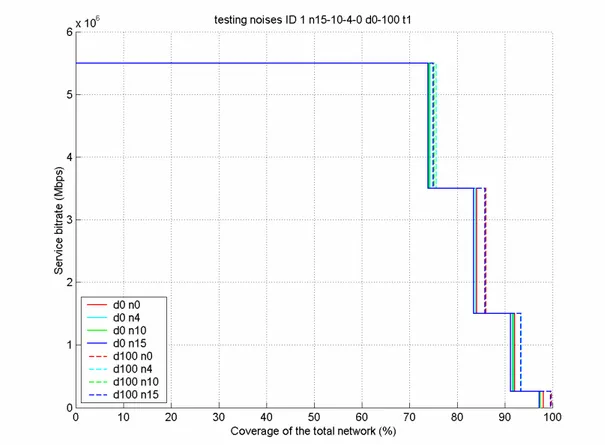
Next figure summarises the results; as we can notice, the lines are very close to one another, showing the low influence of the number of noises.
• HDSL
With HDSL, the coverage increases from 90% up till 97% with an increase of the total network up till 8% .
Now the improvements are consistent since the coverage with the actual ADSL starts to be lower than 90% coverage and so DSM has more room for gaining.
The gain becomes higher as the number of noises increases, but the differences depending on the number of noises are not so big.
Next figure summarises the results; as we can notice, the differences between the dotted lines and the straight lines of the same colour (that depicts the gains) are similar, but now the number of lines significantly influences the total coverage reached. HDSL is a strong noise that significantly influences the performance: DSM level-1 can gain a lot against it.
(Note that the red plot is related to zero noise sources, so only AWGN).
• SHDSL
With SHDSL, the gain is very similar to the one for HDSL, since the PSD levels are more or less the same in our band of interest (see figure n 3 ).
Differently from the previous noises, the best gain is with the minimum number of noises. Anyhow the differences of gain depending on the number of noises are small. (Note that the red plot is related to zero noise sources, so only AWGN).
Figure 7.12: Coverage Gains for Europe with SHDSL depending on number of noise sources
• CONCLUSIONS EUROPE FOR SINGLE NOISES.
The gains of DSM level-1 with respect to the reference ADSL are higher where the noises are worst: with only AWGN and with DSL G9961 the gains are low, while with SHDSL and HDSL we can gain up till 8% of increase in coverage.
The number of noises causes only a small variation in gains for DSM level-1 with respect to normal ADSL for the same noise source.
7.2.4.1.1.1.2 Noise combination
In this paragraph the ETSI noise combination is studied.
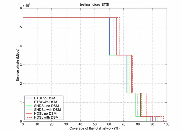
In order to see how the noises combine in the ETSI FB model, we now plot each type of noise with the corresponding number of that source present in the combination, and then we compare the results coming from the ETSI FB combination noise. As expected, the ETSI noise results follow the behaviour of the worst noise in the combination: in the ETSI combination the worst one is the 15 SHDSL lines.
We can conclude that a first good approximation of the results for a noise combination is given by the results of the worst noise.
Following figures support our conclusions:
Figure 7.14: Coverage Gains for Europe with 4 HDSL noise sources
Figure 7.16: Comparison ETSI FB model Vs 4 HDSL & 15 SHDSL
NOTE: a small remark on the last figure is needed, since from that plot it seems that for no DSM the ETSI FB model can have better gains respect to only the SHDSL source. This is due to the distribution used: in the ETSI combination, only the DSL G996 lines have the same distribution as in the single noise. So different topologies have been simulated for the SHDSL as a single source and as a part of the combination: it is only for this reason that the SHDSL is worse than the ETSI FB.
7.2.4.1.2 American Network
Differences in coverage percentage between reference ADSL and full DSM level-1, with different noises tested, are reported in the following table. Comments of them are given below:
While the intermediate gains indicate the number of customers that receive a higher bitrate, the Total Gain indicates the number of additional customers reached when applying DSM. For the American loops it is clearly shown that DSM generally favours the increase for long loops.
Due to that, an operator has to look at the total gain values if he wants to evaluate how much improvements DSM can lead to its customer base.
7.2.4.1.2.1 Noise Effect
In this section we analyse the effects of different noises to the gains between reference ADSL and DSM level-1 applied to all the ADSL lines.
First detailed data on the single noises are presented and then the ETSI combination is studied.
7.2.4.1.2.1 Single noise
• AWGN
Since the coverage with AWGN for American loops is lower than the one for Europe, the improvement that DSM level-1 gives in this case are of 6% increase of the customer base. This higher performance will be a constant in all the American deployments, since DSM privileges gains for long loop and the American lines are longer than the European ones.
Figure 7.17: Coverage Gains for N-America with AWGN
• DSL G9961
As for Europe, with DSL G9961, the coverage increases are of the same order of magnitude as for AWGN: DSL G9961 is only a little bit worse than AWGN.
The gain becomes higher as the number of noises increases, but the differences depending on the number of noises are not so big.
(Note: we remind that the red plots refer to the gains with AWGN only and so are not taken into account for the number of noises).
Figure 7.18: Coverage Gains for N-America with ISDN depending on the number of noise sources
• HDSL
With HDSL, the coverage increases of 16%.
Now the improvements are consistent since the coverage with the reference ADSL starts around 50% and so DSM level-1 has more room for gaining.
The gain becomes higher as the number of noises increases, but the differences depending on the number of noises are not so big.
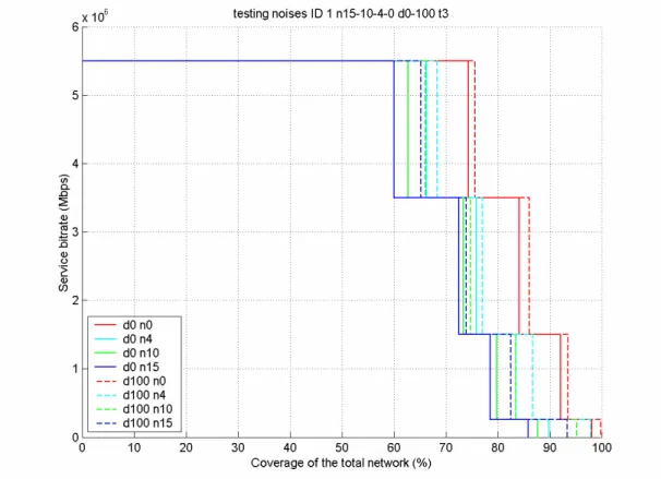
Next figure summarises the results; as we can notice, the differences between the dotted lines and the straight lines of the same colour (that depicts the gains) are similar, but now the number of lines significantly influences the total coverage reached. HDSL is a strong noise that significantly influences the performance: DSM level-1 can gain a lot against it. (Note: we remind that the red plots refer to the gains with AWGN only and so are not taken into account for the number of noises).
Figure 7.19: Coverage Gains for N-America with HDSL depending on the number of noise sources
• SHDSL
With SHDSL, the gain is very similar to the one for HDSL, since the PSD levels are more or less the same in our band of interest (see figure n 3 )
Differently from the previous noises, the best gain is with the minimum number of noises. Anyhow the differences of gains depending on the number of noises are small. (Note: we remind that the red plots refer to the gains with AWGN only and so are not taken into account for the number of noises).
Figure 7.20: Coverage Gains for N-America with SHDSL depending on the number of noise sources
• CONCLUSIONS AMERICA FOR SINGLE NOISES.
The gains of DSM level-1 with respect to the reference ADSL are higher where the noises are worst: with only AWGN and with DSL G9961 the gains are lower, while with SHDSL and HDSL we can gain up till 16% of increase in coverage.
The number of noises gives only a small variation in gains for DSM level-1 with respect to the reference ADSL for the same noise source.
Since DSM level-1 gains more on long lines, the American distribution gains more than the European one: a large number of long lines can be activated thanks to less crosstalk coming from short lines (that apply PBO) and thanks to power reallocation (boosting).
7.2.4.1.2.1.2 Noise combination
In this paragraph the ETSI noise combination is studied for North America.
In order to see how the noises combine in the ETSI standard, we now plot the number and type of noises present in the combination, and then we compare the results coming from the ETSI FB model. As expected, the ETSI noise results follow the behaviour of the worst noise in the combination: in the ETSI combination the worst one is the 15 SHDSL lines.
We can conclude that a first good approximation of the results for a noise combination are given by the results of the worst noise.
Following figures support our conclusions: we plot before the single noises interesting, and then the ETSI FB results together with them.
Figure 7.22: Coverage Gains for N-America with 4 HDSL
Figure 7.24: Comparison ETSI FB model Vs 4 HDSL & 15 SHDSL
7. 2.4.1.3 Conclusions
We can summarise that DSM level-1 compared to the reference ADSL has:
• Gains that depend on the type of noise, but not on the number of noise source. • Best gains with highest noises.
• Best gains for long loop thanks to less crosstalk coming from the short lines that apply power backoff and thanks to boosting (power reallocation on good tones). • Best gains with American loop since its coverage with the reference ADSL is
inferior and since it has more long lines.
• Gains for the combination of noises that follow the behaviour of the worst noise of the combination.
7.2.4.2 Loop Length Reach
For the presentation of the loop length reached, we show our results taking into account the 99% certainty explained in 7.2.1.
We only present the results for the individual noises that belong to the ETSI FB model and the ETSI FB results, since the general information on the behaviour of the gains depending on he quantity of noises and on the type of noises are the same presented in the coverage analysis. With this analysis, we are able to add information on the gain in terms of increase in length thanks to DSM while comparing to the reference ADSL.
Using the 99% certainty plot, we are sure to give with good reliability the maximum length achievable for each service bitrate.
7.2.4.2.1 European Network
Next figures show the loop length reach for our simulation for the European distribution.
Results are given in increasing order of influence of the single noise in the ETSI FB model.
Figure 7.25: Loop Length Reached for Europe with AWGN
Figure 7.27: Loop Length Reached for Europe with 4 HDSL
Figure 7.29: Loop Length Reached for Europe with ETSI FB combination
7.2.4.2.2 American network
Next figures show the loop length reach for our simulation for the American distribution.
Results are given in increasing order of influence of the single noise in the ETSI FB model.
Figure 7.30: Loop Length Reached for N-America with AWGN
Figure 7.32: Loop Length Reached for N-America with 4 HDSL
Figure 7.34: Loop Length Reached for N-America with ETSI FB noise model
7.2.4.2.3 Conclusions
In terms of loop length reached by each service bitrate using the 99% certainty, the gains are of about 500m for the ETSI noise scenario either for Europe either for America.
Using this result and the results coming from the coverage, we can conclude that, as expected, DSM level-1 doesn’t do miracles against the physical limitation of attenuations in the lines (small improvements in loop length reached), but, by reducing crosstalk and boosting on the lines that really need it (the longest lines), it can sensibly increase the coverage (big gains in number of customers added, without reducing the service for customers at shorter lines).
7.2.5 CO/RT
For the CO/RT scenario, we have studied the improvements when applying DSM level-1 only at the RT lines: results coming from this scenario, on one hand show the effects of DSM used only as power Backoff and, on the other hand, quantize the possible gains derived by applying DSM level-1 in the new modems installed at the RT while not changing the old ones at the CO.
We have to mention here that this study is conducted using a loop length distribution for the RT that is not used today in the actual fields. We have used RT lines starting from the second tier of the CO: this is realistic scenario for VDSL. For ADSL this scenario is only a possible deployment that, if used, can give big gains, as the following results will show.
The analysis of CO/RT scenario takes advantages from the results coming from the CO study.
We only analyse the gains for AWGN, since we want only to prove the benefits of applying DSM level-1 in such a scenario: effects of worst noises are imaginable using the information coming from the RT scenario.
7.2.5.1 European Network
We are going to present the coverage gains reached by applying DSM level-1 with respect to the reference ADSL when only AWGN is present in the European network.
The gains are coming from the CO lines that, thanks to PBO applied by the RT lines, can have less crosstalk: a great number of CO lines that with the reference ADSL cannot be activated, now are activated with DSM level-1. To appreciate better this increase, first we plot the gain for all the lines (CO lines and RT lines), then we show the gain referring only to the CO lines.
Figure 7.36: Coverage Gains at CO, for Europe for CO/RT scenario with AWGN
As it is feasible from the previous figures, the gains are really high.
On the plot with total coverage, we can see that in blue and in green always 50% of the lines is at 5.5Mbps : this means in fact that the RT lines are always at 5.5Mbps, so indeed it is more interesting to show only the gains of the CO lines.
While in the reference ADSL the CO lines cannot reach the service bitrate of 5.5 Mbps due to too much crosstalk coming from the RT lines, with DSM level-1 the CO lines can reach now 5.5 Mbps thanks to the PBO applied by the RT lines.
Now the coverage of 5.5 Mbps is again related to the attenuation of the lines and is not anymore completely linked to crosstalk coming from the RT.
With DSM level-1 the total coverage of the entire network (CO/RT lines) is comparable to the total coverage of the entire CO unbunched network previously analysed.
As mentioned in chapter 5, DSM level-1 together with the remote deployment scenario is the solution for substantially increase rate/reach.
7.2.5.2 American Network
We are going to present the coverage gains reached by applying DSM level-1 with respect to the reference ADSL when only AWGN is present in an American network. The gains are coming from the CO lines that, thanks to PBO applied by the RT lines, can have less crosstalk: a great number of CO lines that with the reference ADSL cannot be activated, now are activated with DSM level-1. To appreciate better this increase, first we plot the gain for all the lines (CO lines and RT lines), then we show the gain referring only to the CO lines.
Figure 7.38: Coverage Gains at CO for N-America for CO/RT scenario with AWGN
As it is feasible from the previous figures, the gains are really high.
The coverage increase is higher than in the European case, since, in the American loops, DSM level-1 applied at the RT means an increase in service bitrate from 1,5 Mbps till 5,5 Mbps for the CO lines. This is possible since the long CO lines are really very sensitive to the crosstalk present at their terminal part. Indeed, the attenuation increases with the loop length and so, when the signal arrives at the distance where the RT is positioned in the American loops, this signal is already weak and it is more influenced by the crosstalk. A strong crosstalk kills the signal, while a weak crosstalk only slightly disturbs the CO lines: this explains the big gains found for the American distribution.
7.3 Result Considerations
7.3.1 Characterisation of the topology deviance with respect to the average value
From the experimental results, we have found that in our graphs there is a “transient” region of loop lengths in which we cannot identify directly from the loop length which target bitrate that line would have; the actual bitrate will be influenced by the topology in which that line is present. (Fig.39 and 40 graphically show the problem)
It has been a problem for us because we would like to have a good comparison among all the data and we want to give precise advice for the rate region of DSM level-1.
To solve the problem of comparing data results, we have chosen to use both the average length for each target bitrate and the 99% certainty plots as shown in 7.2.1 (and not min or max length that are related too much to rare cases).
So all the plots for the different parameter values are all referring to the same good criteria and can show statistically the gains in coverage.
But still, since we want to characterize DSM level-1 as much as possible in all its behaviour, and since we would like to give to operators concrete directions on how to use DSM in the real fields, we have investigated if we can predict, just looking at the topology, if a certain line can have a bitrate or another one.
If we can find specific common rules applicable in general, we can propose a proactive approach that can easily be used for the setting of the target bitrates to all the lines of a certain topology, otherwise a reactive approach is needed.
After an investigation on all the topologies used in our simulation, we can say that the main aspects are:
• The noise influence is very big. For AWGN and DSL G996, the deviance respect to the average is maximum 300m, while for HDSL and SHDSL it can reach 1,5 km. Next plots show this feasible difference.
Figure 7.39: Deviance of data points for ISDN
• With respect to the European distribution, the American networks have more problems.
• The problem doesn’t come from the use of DSM level-1: we encounter more or less the same variations both with and without DSM.
• Lines with more or less the same length, but with different bitrate, belong to two different kinds of topologies: lines with lower bitrate belong to topologies that have an higher number of active lines, an higher number of long lines and lengths not so spread as the topologies to which belong the lines with higher bitrate. Follow figures exemplify this sentence.
NOTE: in next figures the lines are coloured depending on the Service Bitrate reached:
- blue is 5,5 Mbps - yellow is 3,5 Mbps - pink is 1,5 Mbps - green is 256 kbps
Example1.
Figure 7.41: Topology investigation for deviance of data points for example 1.
This figure clearly shows how the second topology (that has only two longer lines and a lot of short lines) can set a bitrate of 3.5 Mb/sec to a line of about 3800 m, while the first topology can only set a bitrate of 1.5 Mb/sec for the same length of ∼3800 m because it’s too much influenced by the crosstalk of the other lines (that here are much longer and with many lines around 3800 m).
Example 2.
Figure 7.42: Topology investigation for deviance of data points for example 2.
As we can see from the figure above, a line with a certain length that is at the edge between two Target Bitrates, can set one bitrate or the other one depending on the topology. The topology at the bottom has all the lines active and there are two lines very close to the line of interest: for such a reason, this topology doesn’t reach the higher bitrate of 5.5 Mb/sec that the lines in the other topologies can reach thanks to less crosstalk since not all the lines are active.
Conclusions.
In this section we have characterised how a topology influences the possible bitrate for a certain line length and we have found a general behaviour. But, since we have encountered too many variation factors (noise has a big influence), we cannot give a common rule to follow to set the best Target bitrate in a proactive way.
There are two possible solution:
• The optimal target bitrates for the topology under test could be found preventively with simulations (but this is a waste of time and each time that there is a change in the topology a new simulation is needed).
• The optimal target bitrate are reached in two phases:
1. First the SMC sets the target bitrate coming from our results using the
value coming from the 99% certainty
2. Then an upgrade module can adjust the bitrate on the lines (if any)
7.3.2 Algorithm Convergence
Our algorithm implemented has a problem of convergence both for DSM level-1 and normal bitallocation.
Convergence for DSM.
We noticed that DSM level-1 applied to all the lines (DSM 100%) gives a problem of convergence in about 3% of cases simulated.
That is due to the differences that we have used respect to the real algorithm for the Nash equilibrium: we remind that we have implemented the algorithm in order to find the rate region, so we don’t know which are the target bitrate to set to obtain the convergence. Also our modems iterate all together and not one after another as the Nash equilibrium assumes.
To understand what happens to the lines when applying DSM, we have studied the behaviour of the lines during the iterations. The process is summarised in the following points.
• After enabling their PSD at the standard -40 dBm/Hz, at each iteration the modems calculate their SNR and modify their PSD levels in order to achieve the maximum bitrate attainable with the minimum power.
• A modem stops to change its PSD level when the external noise changes are not significant anymore for giving changes to the bitallocation.
• The first modems to stop the process are the modems that belong to the longest lines: since the FEXT problem decreases with the distance, the PSD level on long lines is prevalently related to the problem of attenuation and once the long lines have calculated their best bitallocation and have applied boosting, they don’t suffer too much from noise changes coming from the other shorter lines and they don’t need to change their PSD level and bitallocation anymore. • The longest lines stop after one iteration, while all the other lines iterate again
setting new values for their PSD and bitallocation.
• One after the other, the modems, starting from the ones that belong to the longest lines, stop to change their profile and after normally 7-8 iterations the
algorithm converges to a stable point: all the modems have reached their best setting.
Problems are present when particular topologies with particular noise conditions have a line close to the edge between 2 bitrate profiles: that lines tries to jump to the higher profile creating new crosstalk to the other lines that have to change the PSD level in order to maintain their bitrate and the process goes into an infinite and periodic loop. The following explanation shows the mechanism.
Next legend shows the colour used in the following figure of the topology.
line disactivated noise Service bitrate 5.5Mbps Service bitrate 3.5Mbps Service bitrate 1.5Mbps Service bitrate 256kbps line under test
We are interested at the line coloured in blue (so line number 9): the line belongs to the rate region of 3,5 Mbps.
The first lines who stop to iterate are the 2 longest and then the other 2 longest among the remaining ones.
100 282431673564 4571 0 2 4 6 8 10 12 14 16 18 20
Step 1. The line under test tries to set 3,5 Mbps and tries to stop to iterate. The other lines adjust their PSD level.
0 1000 2000 3000 4000 5000 6000 7000 0 2 4 6 8 10 12 14 16 18 20 Step 1.
Step 2. Now noise condition are such that the line considered has its maximum attainable bitrate higher than 5,5 Mbps and sets that value, while also the shortest lines continue to adjust their levels.
0 1000 2000 3000 4000 5000 6000 7000 0 2 4 6 8 10 12 14 16 18 20 Step 2.
Step 3. In the next step all the other shorter lines (indicated by an arrow) adjust their PSD level in order to maintain their bitrate: they react to the increase of noise generate by the line that has increased sensibly its PSD level jumping from 3,5 to 5,5 Mbps. 0 1000 2000 3000 4000 5000 6000 7000 0 2 4 6 8 10 12 14 16 18 20 Step 3.
Step 4. Now, since the shortest lines have changed their PSD level, noise conditions slightly change also for the line under test. Its maximum attainable bitrate now is slightly inferior: it cannot reach anymore 5,5 and has to lower sensibly its PSD to achieve 3,5. 0 1000 2000 3000 4000 5000 6000 7000 0 2 4 6 8 10 12 14 16 18 20 Step 4.
So the new changes in noises let the other lines set a lower PSD level again: the new environment will be again good for our line that now can reach again 5,5 Mbps. We are again in step 1 and the loop will run infinitely with this periodicity of four steps.
Solutions:
In order to obtain reliable results, each time that there is a not convergence in our simulations we have downgraded the instable line to the minimum bitrate attainable. In reality this problem can be solved in the same way if we use our algorithm, or can be solved just using the correct target bitrate once that the operators have them from these simulations. Another mechanism that can sensibly reduce this problem is the use of a different value for the MaxAdditNM: if we set a value different from zero, we will have more hysteresis (see 3.1.3) and the instability will be less problematic, but, at the same time, the gain from DSM level-1 will be inferior.
Reference Bitallocation Convergence.
We had also a problem of convergence also for the normal ADSL: in one case we have 2 lines that switch on and off one tone at the same time causing an infinite loop. This reflects the case where there is not enough SNR to allocate bits on a tone if there is another crosstalker, but there is enough SNR without crosstalker.
This problem is partially emphasised by our implementation of monitored tones (see 7.1.1). The lines can measure a vacant tone without self putting energy on it to measure the tone. In reality this cannot happen : both modems will put energy on the tone in order to monitor it and sense each others crosstalk. Due to this crosstalk, there is not enough energy for any of them to put a bit on this tone. For this problem we don’t have to mention any solutions since this defect anyhow doesn’t interfere with the offered bitrate, it is a problem not caused by DSM, but it’s mainly caused by our approximations.