5 Modelling
Since the geometry of the furnace is far to be similar at all standard mixing models, a model developed by K. Takenaka20 at University of Birmingham was used to compare experimental data with analytical results. This model is performed for Rushton turbine and cylindrical vessel with baffles, and is based on the computation of gas hold-up and the model for gas power characteristics. Naturally some geometrical parameters have been modified according to the different vessel shape.
5.1 The Computation of Gas Holdup
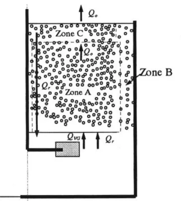
The proposed model has divided stirred reactors, equipped with turbine inducing radial flow, in three zones; Zone A, the main body of the tank where the gas hold-up has been calculated, Zone B where a low void fraction is present because of the presence of baffles and Zone C where the gas flow rate coming from Zone A is shared in the recirculated flow rate and in the flow rate leaving the tank.
The present model used to compute gas hold-up is based on the mass balance on the gas entering and leaving Zone A and can be used only if the gas recirculation exists, therefore can not be used if flooding conditions occur. As shown in Figure 5-1, there are two gas flow rates entering the zone, labelled with
Q
r andQ
VG and a single flow rate leaving the zone, labelled withQ
o.The gas flowrate
Q
VG is the gas volumetric flow rate through the sparger,Q
r, is the gas volumetric flowrate recirculated to the impeller andQ
o is the gas volumetric flow rate leaving Zone A.To evaluate the recirculated gas flow rate,
Q
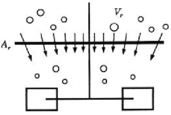
r, the fluid dynamics of the zone above the impeller has to be analysed.In this model the zone below the impeller has not been taken into account because usually gas hold-up in it is absolutely lower than that in the Zone A above the impeller. A schematic diagram of the impeller is shown in Figure 5-2.
The volumetric gas flowrate,
Q
r,
can be computed as a product ofthe surface area,
A
r, (see Figure 5-2), the void fraction above theimpeller,
e
r, and the absolute velocity of the gas phase in that zone,V
r:The velocity
V
r, taking into account of the buoyancy force, can becomputed as:
where
V
b, is the bubble rising velocity in stagnant liquid,f
is the Flownumber and, therefore
, f N D
3 is the mixture flow rate flowing through the impeller.The volumetric gas flow rate
Q
o,
can be computed as a product ofthe surface area of the Zone A,
A
a, the void fraction in that zone,e,
and the absolute velocity of the gas phase in that zone,
V
a, r r r rV
A
Q
=
⋅
⋅
ε
Eq. 5-1 b r rV
A
D
N
f
V
=
⋅
⋅
−
3 Eq. 5-2Because the mean axial velocity of the liquid phase, calculated on the cross section, is nil, the velocity
V
a can be calculated as,Finally the following relation is derived from the mass balance, on the gas phase in Zone A,
and therefore:
Gas hold-up above impeller remains approximately constant changing cavity shape from vortex to large “3-3” structure20. Taking into account this experimental evidence it is possible to assume that
e
r, is constant independently from the working conditions. Finally,using the following labels:
ε
⋅
⋅
=
a a oV
A
Q
Eq. 5-3 b a r VG aV
A
Q
Q
V
=
+
+
Eq. 5-4 VG r oQ
Q
Q
=
+
Eq. 5-5
−
⋅
⋅
⋅
+
=
=
⋅
⋅
+
⋅
⋅
⋅
⋅
−
+
b r r r VG a b a r r b r VGV
A
D
N
f
A
Q
A
V
A
A
V
A
D
N
f
Q
3 3ε
ε
ε
Eq. 5-6 a b r r b r VG r r b r VGA
V
A
V
D
N
f
Q
A
V
D
N
f
Q
⋅
+
⋅
⋅
−
⋅
⋅
⋅
+
⋅
⋅
−
⋅
⋅
⋅
+
=
ε
ε
ε
ε
ε
3 3 Eq. 5-7the Eq. 5-7 assumes the final form:
The product
f·e
r has been empirically derived equal to 0.04, this resultagrees with published experimental data. In fact, if a Rushton turbine is used, the flow number,
f
, can be assumed equal to 0.75 (Revili, 1982) and therefore the void fraction,e
r,
results equal to0.04/0.75˜0.05.
The surface area
A
r is a function of the impeller size,D
. Presentanalysis is based on the assumption that:
4
2 3 *T
D
N
f
Q
V
VG r m⋅
⋅
⋅
⋅
+
=
π
ε
Eq. 5-8
⋅
⋅
⋅
=
4
2T
A
V
V
r r b oπ
ε
Eq. 5-9
⋅
⋅
−
⋅
=
4
2 1T
A
A
V
V
b a r rπ
ε
Eq. 5-10 1 * *V
V
V
V
m o m+
−
=
ε
Eq. 5-11where
C
1 has been empirically derived equal to 1.31.The surface area
A
a, has to be evaluated as the difference of thetank surface area minus the area of a zone B that presents low void fraction. Therefore the surface area
A
a can be empirically computedas:
where the length
W
is the width of the vessel andL
the length where a high amount of rising bubbles are present.Finally it is necessary to compute the bubble rising velocity,
V
b. It iswell known that this velocity is a function of bubble dimension and of the physical properties of working fluids. From the theoretical point of view, the bubble size depends also on the operating conditions such as stirrer speed and impeller diameter and also on the characteristics of solutions. However, as shown also by Takenaka20, if the stirrer speed is sufficiently great, the influence of agitation on the bubble size stabilises. Consequently the bubble diameter can be considered as a function of the Eotvos number,
Eo
crit :where
?
L is the density of the liquid phase,s
the surface tension andg
the acceleration of gravity.
4
2 1D
C
A
r⋅
⋅
=
π
Eq. 5-12L
W
A
a=
⋅
Eq. 5-13σ
ρ g
d
Eo
L crit⋅
⋅
=
2 Eq. 5-14Van Dierendonck et al., analysing the behaviour of three pure liquids, water, cyclohexane and n-hexane, empirically suggested a constant value of
Eo
crit equal to 0.3. This value, according to the analysis byClift et al.21 on the single bubble behaviour, is fairly corresponding to
the transition from Spherical to Ellipsoidal/Wobbling regime, for air/water system. Therefore, the experimental data by Van Dierendonck et al. suggest that, if the stirrer speed is sufficiently great, the bubble size can be calculated as the critical bubble dimension corresponding to the transition from Spherical to Ellipsoidal/Wobbling regime.
The critical Eotvos number,
Eo
crit, is not a constant21, depending onthe physical property. Namely if not water-liquid systems, the critical Eotvos number,
Eo
crit, assumes a different value which can becalculated as a function of the property group M, defined as:
Finally, in present analysis, to evaluate the bubble size change relative to the physical properties of the working fluids, the transition between Spherical/Ellipsoidal regimes suggested by Clift et al. (1978) has been utilised. It is necessary to point out that, if the stirrer speed is lower than the critical value evidenced by Van Dierendonck et al. (1968), bubble size is underestimated by using Eq. 5-14, therefore bubble rising velocity and gas hold-up can be underpredicted by Eq. 5-11.
From the knowledge of the bubble size, it is easy to calculate the bubble rising velocity only if relatively inviscid liquids are used. As
(
)
2 3 4 L G L Lg
M
ρ
σ
ρ
ρ
µ
⋅
−
⋅
⋅
=
Eq. 5-15pointed out by Hartunian and Sears (1957), it is necessary to distinguish between “fast fluids” and “slow fluids” because they present a completely different behaviour. The group that allows to separate these two categories is the property group M (see Eq. 5-15). These authors showed that the threshold is in the range of
M
= 10-8-10 -7, therefore in present analysis the critical va1ueM
= 1O-8 has been utilised.If the property group is lower than the critical value
M
crit a lot ofdifferent equations can be used to predict the bubble rising velocity Vb. In present analysis, because the bubble size in inviscid fluids is
approximately equal to 3 mm, the bubble rising velocity in stagnant fluid,
V
b,
has been computed as:where the critical Weber number,
We
c r i t, can be assumed equal to3.46, as suggested by Brodkey22.
d
We
V
L crit b⋅
⋅
=
ρ
σ
Eq. 5-165.2 The Model for Gassed Power Characteristics
In order to evaluate the aerated power number, it is necessary to know exactly the gas flow rate that flows into the impeller. Therefore one of the goals in the present model is to evaluate the gas recirculation. Then, starting from the mass balance the aerated power number for single impeller will be evaluated and finally the transition between loading and flooding conditions will also be determined using similar approach.
The model for the recirculated gas assumes that the two-phase mixture in the stirred tank is homogeneous, in other words, that there is no gradient of the gas-hold up throughout the vessel.
Bubble flow rate inside the agitated vessel is determined by bubble
Figure 5-3: Schematic diagram of bubbles and liquid motion in a stirred tank with single impeller
terminal velocity and liquid velocity (see Figure 5-3). If the fluid velocity is less than the bubble rising velocity all bubbles move to the top of the vessel and the recirculation is absent. Otherwise if the liquid velocity,
V
l, overcomes the bubble rising velocity,V
b, the gasrecirculation flow rate is proportional to the gas hold-up, e, and to the effective gas velocity,
V
g. Accordingly, the flow rate of recirculatedgas,
Q
r, which come back into cavity with freshly sparged gas can beevaluated as
where A is the cross section for recirculation and has been defined as
In this approach, it has been assumed that the main gas recirculation comes from above the impeller.
The effective liquid and gas velocities,
V
l, V
g, can be computed fromthe following continuity equation as functions of the mean velocity,
V
m, and the bubble rising velocityV
b,Where and finally
(
)
≤ = > − ⋅ ⋅ = ⋅ ⋅ = b l b l b l g r V V Q V V V V A V A Q if 0 if ε ε Eq. 5-17 π ⋅ = 2 2 D A Eq. 5-18(
−ε)
+ ⋅ε ⋅ = l g m V V V 1 Eq. 5-19 b l g V V V = − Eq. 5-20ε
⋅
+
=
m b lV
V
V
Eq. 5-21(
−ε)
⋅ − = m b 1 g V V V Eq. 5-22The mean velocity can be expressed as
where the mixture flow rate
Q
m is proportional to the stirrer speedN
and to the
D
3where a is a proportionality coefficient. Finally, Eq. 5-17 can be expressed as
The final form of the ratio between the recirculated gas flow rate and the gas flow rate coming from the sparger becomes:
The equation shows that the ratio of
Q
r/Q
VG is a strict function of gashold-up, e.
From the analysis of the experimental recirculation data for a single disc
a
was found to be equal to 0.7.It is well known that the power consumption in a single-phase system can be calculated from:
It is also well known (Mc Cabe et al.23, and Harnby et al .24) the power number,
Po
, is constant in turbulence region, irrespective of the stirrerA Q V m m = Eq. 5-23 3 D N a Qm = ⋅ ⋅ Eq. 5-24
(
ε
)
ε
π
ε
(
ε
)
ε
⋅
⋅
⋅
−
⋅
−
=
⋅
⋅
−
⋅
⋅
⋅
−
⋅
=
1
4
1
2 3 3D
V
ND
a
V
A
D
N
a
A
Q
r b b Eq. 5-25(
)
VG b VG VG rQ
D
V
Q
ND
a
Q
Q
⋅
−
⋅
⋅
⋅
⋅
−
⋅
⋅
=
4
1
2 3π
ε
ε
ε
Eq. 5-26 5 3D
N
Po
P
=
ρ
L Eq. 5-27speed. Frijlink et al.25 have proposed the power consumption in an
ungassed suspension:
where ρeffSL and
Po
SL are the effective density of slurry and the modified power number which accounts for the ratio ρeffSL/ρLrespectively. Similar, for power consumption in a gas-liquid system, one may write:
Therefore the relationship between the power consumption under aerated and unaerated condition can be obtained:
Finally, in order to evaluate the ratio between the ungassed and the gassed power consumption, it is necessary to evaluate the effective fluid density surrounding the impeller. It is apparent that the effective density cannot be presented as the mean fluid density throughout the tank due to the presence of gas cavity. Here, it assumes that the effective density is the same with the mean fluid density in the impeller region. The mean fluid density inside the turbine,
ρ
GL, depends upon the dimension of the cavities behind the blades of impeller and upon the density of the gas-liquid mixture.5 3 5 3
D
N
Po
D
N
Po
P
SL=
ρ
effSL=
SLρ
L Eq. 5-28 5 3 5 3D
N
Po
D
N
Po
P
g=
ρ
effGL=
GLρ
L Eq. 5-29Po
Po
P
P
GL L effGL g=
=
ρ
ρ
Eq. 5-30(
)
L G GL effGL ρ xρ x ρ ρ = = + 1− Eq. 5-31where
x
indicates the volumetric gas void fraction including the cavity derived behind the blade in the impeller region for gas-liquid system. By introducing a dimensionless cavity size,β
t, as following(see also Figure 5-4):
it is possible to define the mean density of the mixture,
ρ
GL:where
ρ
G andρ
m are the gas density and the mean density of the fluid flowing into the turbine, respectively. If the slip velocity between the gas and liquid phases derived by the turbine can be neglected, it2 1 2
L
L
L
t=
+
β
Eq. 5-32(
t)
G t m GLρ
β
ρ
β
ρ
=
1
−
+
⋅
Eq. 5-33is possible to evaluate the gas hold-up of the gas/liquid mixture into the turbine,
ε
m, asand consequently
Therefore x in Eq. 5-31 can be expressed:
and consequently Eq. 5-31 becomes:
However, in actual fact, the effective density ρeffGL will generally not be equal to the mean density or to the liquid density
ρ
L. It is well known that the power drawn is extremely affected by the cavities formed behind the blades. The presence of the cavity must be taken into consideration to obtain the effective density necessary to evaluate the power drawn. Hence a coefficient is added to the term on the cavity in Eq. 5-37 in order to express the effect of cavities. Therefore the effective density can be presented:where
C ’
indicates the effect of the cavity formation on the effective density in gas liquid. Moreover many papers have been published onm r VG m
Q
Q
Q
+
=
ε
Eq. 5-34(
)
L m G m ε ρ ε ρ ρ = 1− ⋅ + ⋅ Eq. 5-35 t t m mx
=
ε
−
ε
β
+
β
Eq. 5-36(
m m t t)
G(
(
m m t t)
)
L GL effGL ρ ε ε β β ρ ε ε β β ρ ρ = = − + + 1− − + Eq. 5-37(
m m t t)
G(
(
m m t t)
)
L effGL ε C ε β C β ρ ε C ε β C β ρ ρ = − ' + ' + 1− − ' + ' Eq. 5-38the influence of the cavity structure on the power consumption. It is intuitive that the dimension of them depends on the gas flow rate that flows under the impeller. In the present study the following simplifying hypothesis is assumed:
where
C”
is a proportionality coefficient. This assumption will be easily removed when more information on the cavity size becomes available.From the previous assumption, the following equation is derived:
(
Q
C
'
''
=
C
'
⋅
C
''
)
and finally
This equation can be used to predict the power consumption if the turbine is not flooded.
m t
C
ε
β
=
"
⋅
Eq. 5-39(
m)
L(
m)
G(
m)
m effGL ε ρ C ε ρ C ε C ε ρ = 1− ⋅ ⋅ 1− ' ''⋅ + ⋅ 1− ' ''⋅ + ' '' ⋅ Eq. 5-40(
) (
)
(
m)
m L G m m gC
C
C
P
P
ε
ε
ρ
ρ
ε
ε
⋅
−
⋅
+
⋅
−
⋅
+
⋅
−
=
1
1
'
''
1
'
''
'
''
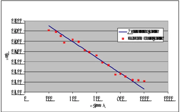
Eq. 5-41Finally, the model described above has been applied at 3PBT30 impeller; in Figure 5-5 is shown the comparison between experimental work and the analytical data found from Eq. 5-41, where
e
m isperformed from Eq. 5-11. The following values have been used for all other parameters.
Table 5-1: Modelling values
Q
VG[ m
3/s]
εr
[ -]
f
[ -]
D
3[ m
3]
V
b[m/s]
A
r[ m
2]
Aa
[ m
2]
C'''
[ -]
1,67E-05 0,05 0,57 1,04E-04 0,27 1,73E-03 0,04 170
From Figure 5-5 is clear how this model correctly works also with the geometry used in this thesis.
0,300 0,400 0,500 0,600 0,700 0,800 0,900 1,000 0 200 400 600 800 1000 1200 N (rpm) Pg/P Calculated data Experimental data