POLITECNICO DI MILANO
SCUOLA DI INGEGNERIA CIVILE, AMBIENTALE E TERRITORIALE
MASTER PROGRAMME IN ENVIRONMENTAL AND GEOMATIC ENGINEERING
AN EVALUATION OF MODFLOW_USG
Master Dissertation by:
PARISA FALAKDIN
Student ID N: 863171Supervisor:
Prof. LUCA ALBERTI
Co-supervisors:
Ing. Angelo Ortelli
Ing. Matteo Antelmi
I |POLITECNICO DI MILANO
Acknowledgment
It is a genuine pleasure to express my deep sense of thanks and gratitude to Professor Luca Alberti for providing me the opportunity of working and learning along with his professional team.
I sincerely thank Professor Ivana La Licata for her keen interest and guidance at different stages of this research.
I owe a deep sense of gratitude to Angelo Ortelli for providing such nice support and guidance. His prompt inspiration, timely suggestion, enthusiasm, and dynamic have enabled me to accomplish this task.
In addition, a thank you to Matteo Antelmi for providing me with the required information and guidance during this work.
In the end, it is my privilege to thank my family for their constant support and encouragement throughout my graduate study.
II |POLITECNICO DI MILANO
Abstract
The majority of software for groundwater modeling is based on finite difference and finite element methods. In 2013, the United States Geological Survey ( USGS) released a new version of MODFLOW, called MODFLOW-USG, in order to support UnStructured Grids. Soon enough, graphical user interface (GUI ) provided the new version of Groundwater Vistas (ver. 6) in order to support MODFLOW-USG software packages.
In the first part of this thesis, a study area, previously modeled using a structured version of MODFLOW (i.e. MODFLOW2000), is developed in MODFLOW-USG in order to evaluate its new features and capabilities in comparison with the older version.
In the second part of the study, MODFLOW-USG is applied to another study area, previously modeled with MODFLOW-2005, in order to simulate the transport of heat through a borehole heat exchanger using the new transport package provided by USG and make a comparison with the results obtained through MODFLOW-2005. Different approaches for the grid design and the u-pipe representation are applied for finding the best possible solution.
The results of the comparisons between structured and unstructured versions of MODFLOW show that for simple problems (as the one of the first part of this study), MODFLOW-USG could provide flexibility in grid design resulting in fewer grid cells and consequent faster running process. However, the second part of this study, where a very refined grid is required due to the complexity of the problemMODFLOW-USG turns out to be not able to provide the correct results with an unstructured grid, while the grid generation is still better with MODFLOW-USG.
Keywords: MODFLOW-USG, MODFLOW, CLN, quadtree grid, nested grid, control volume finite difference, finite difference, geothermal energy, borehole heat exchanger.
Sommario
La maggior parte del software per la modellizazione delle acque sotterranee si basa sui metodi di differenze ed elementi finiti. Nel 2013, lo United States Geological Survey ha rilasciato una nuova versione di MODFLOW, chiamata MODFLOW-USG, al fine di supportare le griglie non strutturate. Graphical user interface (GUI ) ha fornito la nuova versione di Groundwater Vistas (versione 6) per supportare i pacchetti software MODFLOW-USG.
Nella prima parte di questa tesi, un'area di studio, precedentemente modellata utilizzando una versione strutturata di MODFLOW (MODFLOW2000), è sviluppata in MODFLOW-USG per valutare le nuove funzionalità rispetto alla versione precedente.
Nella seconda parte dello studio, MODFLOW-USG è applicato a un'altra area di interesse, precedentemente modellata con MODFLOW-2005, per simulare il trasporto di calore attraverso uno borehole heat exchanger utilizzando il nuovo pacchetto di trasporto fornito da USG e fare un confronto con i risultati ottenuti attraverso MODFLOW-2005. Diversi approcci per la progettazione della griglia e la rappresentazione della U-pipe vengono applicati per trovare la migliore soluzione possibile.
I risultati dei confronti tra versioni strutturate e non strutturate di MODFLOW mostrano che per problemi semplici come quello della prima parte di questo studio, MODFLOW-USG potrebbe fornire flessibilità nella progettazione della griglia con conseguente riduzione delle celle della griglia ed un conseguente processo di esecuzione più veloce.
Tuttavia, la seconda parte di questo studio, dove è richiesta una griglia molto raffinata a causa della complessità del problema MODFLOW-USG risulta essere in grado di fornire risultati corretti con una griglia non strutturata, mentre la generazione della rete è ancora migliore con MODFLOW-USG.
Keywords: MODFLOW-USG, MODFLOW, CLN, griglia quadtree, griglia nested, control volume finite difference, finite difference, energia geotermica, scambiatore di calore a pozzo.
1 INTRODUCTION ...13
2 Theoretical Framework ...15
2.1 Scientific Contest ………...15
2.2 MODFLOW and MODFLOW-USG………16
2.2.1 MODFLOW……….16 2.2.2 MODFLOW-USG………...17 2.2.3 CLN Package……….25 2.2.4 BCT Package……….27 2.2.5 PCB Package ………29 2.2.6 Solver ……….29
2.2.7 River and Stream Packages………..30
3 The Simulation of Plane Zone with MODFLOW-USG ... 33
3.1 Case Study Description ... 33
3.1.1 The purpose of the first simulation with MODFLOW-USG... 36
3.2 Implementation of MODFLOW-USG for a Plane Land Zone……….37
3.2.1 Grid ... 37
3.2.2 Top and Bottom Elevation ... 39
3.2.3 Hydraulic Conductivity ... 41 3.2.4 Porosity ... 42 3.2.5 Recharge ... 43 3.2.6 Analytical element ... 44 3.2.7 Initial Condition ... 45 3.2.8 Boundary Condition ... 45
3.2.9 Difficulties of the Implementation ... 48
3.3 The Obtained Results from the Simulation of Plane Zone……….…. 49
3.3.1 Results of the Simulation of the River Using RIV and SR Packages ... 53
4 The Simulation of the Geothermal Model MODFLOW-USG ...58
4.1 Geothermal Energy systems ... 58
4.1.1 Heat Trasport Equation………..58
4.1.2 Ground Source Heat Pump………..60
4.2 Case Study of the Geothermal Model ... 61
4.2.1 The purpose of the geothermal model………..62
4.3 Implementation of the Geothermal Model with MODFLOW-USG ... 63
4.3.1 Previous Simulation with MODFLOW-2005………..63
4.3.2 Geothermal System Simulation with Un-structured Grid……….67
4.3.3 Geothermal System Simulation with AlgoMesh.………..………..68
4.3.4 Geothermal System Simulation with CLN………..………..72
4.3.5 MODFLOW-USG Transport………...………77
4.4 Results of the Simulation of the Geothermal System in MODFLOW-2005 and MODFLOW-USG ... 78
4.4.1 MT3DMS Package………78
4.4.2 BCT-PCB Package………...80
4.4.3 The Contour-Line Comparison of Temperature………..83
5 Conclusions ...85
III |POLITECNICO DI MILANO
LIST OF FIGURES
FIGURE 1. Ghost node location with respect to the cell center (Panday, 2013) ………20
FIGURE 2. Different types of un-structured grid (Panday, 2013) ………. ....21
FIGURE 3. Nest numbering scheme (Panday, 2013) ………22
FIGURE 4. The position of ghost node around a nested grid (Panday, 2013) ………...23
FIGURE 5. Layer numbering in parent layers and sublayers (Panday, 2013) ………...24
FIGURE 6. Nested grid representation……….….25
FIGURE 7. Quadtree refinement representation………...……...…...25
FIGURE 8. Connected linear network (Panday, 2013) ……….26
FIGURE 9. The study area of the plane zone………...33
FIGURE 10. Base map of the plane zone. ………...……34
FIGURE 11. Geological map of the plane zone relating to the first layer………...…...……35
FIGURE 12. Geological map of the plane zone relating to the second layer………...……...…….35
FIGURE 13. Geological map of the plane zone from the cross-sectional view……….…..…..36
FIGURE 14. The base map which is added to the model………..………...37
FIGURE 15. Grid discretization in MODFLOW2000 model………...………..37
FIGURE 16. Grid discretization in MODFLOW-USG model………...……….39
FIGURE 17. Top elevation zones in the model………..40
FIGURE 18. Hydraulic conductivity zones in the model………...………..…………42
FIGURE 19. Porosity zones in the model………..………..………43
FIGURE 20. Analytical well location is shown on the base map………...……..44
FIGURE 21. Well information window………..……….44
FIGURE 22. Flow information of the stream cells……….……..48
FIGURE 23. Computed head values for the simulation of MODFLOW-USG vs MODFLOW2000……….. 50
FIGURE 24. Water table contour lines for the simulation of MODFLOW-USG vs MODFLOW2000 ……….………50
FIGURE 25. Mass balance summary for the simulation of MODFLOW2000………51
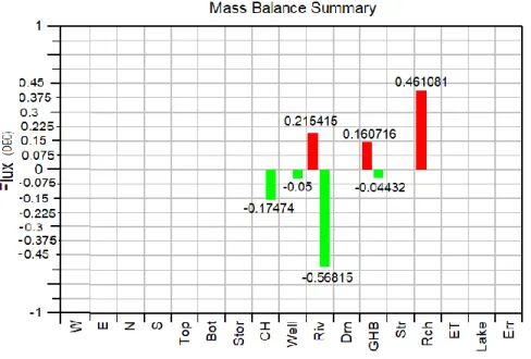
FIGURE 26. Mass balance summary for the simulation of MODFLOW-USG………..…51
FIGURE 27. The comparison between contour lines of RIV and STR packages ………55
FIGURE 28.Operation of a GSHP in the heating mode ………...61
FIGURE 29. The horizontal cross-section of a typical BHE ………62
FIGURE 30. Plan view (a) and section (b) of the model implementation in MODFLOW ……….……64
FIGURE 31. Cells representing the pipe inlet and outlet ……….64
FIGURE 32. 3D representation of the inserted BHE. ……… 67
FIGURE 33. The cross-sectional view of BHE in the model ………..……….67
FIGURE 34. Delaunay triangulation ………69
FIGURE 35.An example of Voronoi grid overlaid on its dual Delaunay triangulation (AlgomeshUserGuid, 2016)…...70
FIGURE 36. The study area covered with AlgoMesh grids ………71
FIGURE 37. The AlgoMesh grid in the area of the BHE ………..………. 71
FIGURE 38.Head variation obtained from AlgoMesh gridding in MODFLOW-USG ……….……72
FIGURE 39. MODFLOW-USG CLN conduit options window (CLN option tab) ……….…..73
FIGURE 40. MODFLOW-USG CLN conduit options window (Connections tab)………..….……74
FIGURE 41. CLN polyline connections shown with circles ………...75
FIGURE 42. The cross-sectional view of head contour lines for CLN polyline approach……….…76
FIGURE 43. The cross-sectional view of the u-pipe using CLN wells and CLN polylines ………76
FIGURE 44. The plane view of the 13th layer showing the CLN polyline connecting two CLN wells ..………77
FIGURE 45. The plane view of the first layer in the simulation done with MT3DMS package………….………78
FIGURE 46. The plane view of the 6th layer in the simulation done with MT3DMS package ………..…79
FIGURE 47. The plane view of the 13th layer in the simulation done with MT3DMS package………..…..79
FIGURE 48. The cross-sectional view of the simulation done with MT3DMS package …..……… 80
XI |POLITECNICO DI MILANO
FIGURE 50. The plane view of the 6th layer in the simulation done with BCT-PCB package………81
FIGURE 51. The plane view of the 13th layer in the simulation done with BCT-PCB package ………..………82
FIGURE 52. The cross-section view of the simulation done with BCT-PCB package………..………82
FIGURE 53. The contour-lines of the heat transport ……….………...…..83
LIST OF TABLES TABLE 1. Bottom elevation values ... 40
TABLE 2. Hydraulic conductivity values ... 41
TABLE 3. Porosity values. ... 42
TABLE 4. Obtained result for the simulation of MODFLOW-USG vs MODFLOW2000 ... 49
TABLE 5. Mass balance table (MODFLOW2000) ... 52
TABLE 6. Mass balance table (MODFLOW-USG) ... 52
TABLE 7. Statistic summary comparison between RIV and STR packages ... 54
TABLE 8. Mass balance table (RIV package)... 55
TABLE 9. Mass balance table (STR package) ... 56
TABLE 10. Parameter assigned to the model for aquifer and borehole ... 65
13 |POLITECNICO DI MILANO
1 Introduction
Groundwater is one of the main natural resources, which supports human health, economic development, and ecological diversity. Overexploitation and unabated pollution of this vital resource are threatening our ecosystems and even the life of future generations [1]. In order to manage water resources and take accurate decisions towards long-term sustainable yield from water systems, we need a better understanding of the real field conditions. For this purpose, groundwater modeling is used as a powerful tool for water resources management, groundwater protection, and remediation.
A model represents reality in a simple way. It is a tool for understanding the system and its behavior towards the environment. Models are used for prediction purposes before the implementation of a project or a remediation scheme. Nowadays, a variety of tools have been designed for the modeling purposes which are constantly improving. All these advancements follow similar objectives such as minimizing the errors, shortening the time of data processing, and simplifying the application process.
Groundwater models can be categorized into physical, analog, and mathematical. A mathematical model simulates groundwater flow and/or solute fate and transport indirectly by means of a set of governing equations to represent the physical processes that occur in the system [2]. Mathematical models are either analytical or numerical. Analytical methods mostly are used for simple cases, while in the numerical methods, more data can be inserted into the model and they are useful for more complicated problems.
In 1988, MODFLOW package was released and it could make a reliable platform for engineers in mathematical modeling of groundwater. In 2013, the USGS (United States Geological Survey) website released a new version of MODFLOW which is called MODFLOW-USG with un-structured grids that is based on Control Volume Finite Difference (CVFD) formulation while the structured version of MODFLOW is based on Finite Difference (FD) approach.
In the first part of this work, a synthetic model is simulated using MODFLOW-USG. The same model has been represented previously by MODFLOW2000. The objective is to evaluate the new features embedded in MODFLOW-USG and also to provide a comparison between the results of the simulations obtained by the two versions. In the second part of this work, a geothermal system, previously simulated by MODFLOW-2005, is considered. The objective is to provide an easier approach for the same simulation in MODFLOW-USG by evaluating different gridding systems, and also by using Connected Linear Network (CLN) and MODFLOW-USG transport packages. The results of the transport model are brought versus MODFLOW-2005.
15 |POLITECNICO DI MILANO
2 Theoretical Framework
2.1 Scientific Contest
The complex nature of environmental problems and of the geological systems requires the use of mathematical models for simulating the flow of groundwater in these heterogeneous media [3].
Groundwater flow modeling tools have been developed during the last decades in order to simulate boundary condition, hydraulic properties, initial condition data and real field observation in the most possible accurate way [3].
MODFLOW is one of the most popular groundwater flow modeling programs which has been applied to a variety of projects worldwide in order to make reliable and accurate groundwater simulation.
Recently, a new version of MODFLOW, called MODFLOW-USG (un-structured grid), was developed to support a wide range of structured and unstructured grid types, including nested grids and grids based on prismatic triangles, rectangles, hexagons, and other cell shapes [4].
Therefore, MODFLOW-USG is a relatively new platform and only a few types of research have been carried out for the examination of the efficiency and accuracy of this new version over the traditional ones. This thesis is subjected to evaluate MODFLOW-USG capabilities.
2.2 MODFLOW and MODFLOW-USG
MODFLOW and MODFLOW-USG characteristics are described in this section:
2.2.1 MODFLOW
MODFLOW is a computer program that is able to solve the three-dimensional ground-water flow numerical equation for a porous medium with the finite-difference method. MODFLOW was documented at 1984 by McDonald and Harbaugh. Since then different advancement and updates have been done to improve the capabilities of the program.
The finite difference is a numerical method for solving systems of differential equations that describe mass, momentum, and energy balances. The differential equations contain a function and its derivatives. The function normally describes a physical quantity and the derivatives express the variation of that physical quantity. The function is estimated by a finite difference approximation. In Finite Difference method, the continuous variables are replaced by discrete variables. Therefore, instead of finding the solution for the whole continuous domain, the solution is determined at discrete step points.
MODFLOW simulates the transport of contaminants using MT3D package. MT3D is a three-dimensional module for transport which is developed by Alabama University [5]. MT3D has various capabilities and options which enables the simulation of contaminants in groundwater flow. There are three main classes of transport solution techniques that are written in one code which are the standard finite-different method; the particle-tracking-based Eulerian-Lagrangian methods; and the high order finite-volume TVD method. There is no single numerical technique that can cover all transport conditions, therefore, the combination of the mentioned solution techniques can be the best approach for solving the vast transport problems and provide an acceptable degree of accuracy and efficiency [6].
17 |POLITECNICO DI MILANO The standard MODFLOW versions simulate groundwater flow using structured rectangular grids [7]. For a structured grid, each cell is specified by addressing the corresponding layer, row, and column. One limitation concerning this type of gridding is that irregular domains cannot simply be fitted by rectangular grids elements. Another important restriction is that it is difficult to refine the grid resolution only in the area of interest [4].
Groundwater Vistas (GV) is a Graphical User Interface that supports MODFLOW software packages. The latest version of Groundwater Vistas (ver. 7), which is used in this work, is largely similar to its previous ones. One of the biggest new features in version 7 is the incorporation of triangular and Voronoi grids for MODFLOW-USG [4].
2.2.2 MODFLOW-USG
MODFLOW-USG was developed to support un-structured grid types to improve the flexibility in the grid design. The ability to use cell shapes other than rectangles is an important feature in MODFLOW-USG. Cells can be variably shaped including grids based on prismatic triangles, rectangles, hexagons, and other cell formats. The grids are elastic in MODFLOW-USG which can be useful to provide concentrated resolution along rivers, wells, and the area of interest. It can also enable the sub-discretization in individual layers in order to describe the hydro-stratigraphic units in a better way.
In MODFLOW-USG, cells must be prismatic in a vertical direction. Cells can be considered as a group for each layer and ease the processing or divide as a sublayer.
MODFLOW-USG is based on control volume finite difference (CVFD) formulation, therefore, each cell can be connected to an arbitrary number of adjacent cells [4]. This method enables each layer to have its own discretization.
Tightly coupling of multiple hydrologic processes is a new framework for MODFLOW-USG. The framework includes the cells for all processes and allows individual MODFLOW-USG processes to add to the global conductance matrix.
The fluxes between cells within a process are displayed as well as the cells of other processes. The CVFD formulation accommodates this unstructured framework of tightly coupling flow processes as well as of allowing flexibility in cell geometry and connectivity within processes [4]. The general form of the CVFD balance equation is as follow:
∑𝑚∈ƞ𝑛𝐶𝑛𝑚(ℎ𝑚− ℎ𝑛) + 𝐻𝐶𝑂𝐹𝑛(ℎ𝑛) = 𝑅𝐻𝑆𝑛 (1)
Where
𝐶𝑚𝑛 is the inter-cell conductance between cells n and m, ℎ𝑚 and ℎ𝑛 are the hydraulic heads at cells n and m,
𝐻𝐶𝑂𝐹𝑛 is the sum of all terms that are coefficients of ℎ𝑛 in the balance equation for cell n, and
𝑅𝐻𝑆𝑛 is the value of the balance equation for the right side of the equation.
The time-dependent storage term included in the 𝐻𝐶𝑂𝐹 𝑛and 𝑅𝐻𝑆𝑛 terms may be
expressed for nonrectangular cells in terms of the cell volume as
𝐻𝐶𝑂𝐹𝑛 =−𝑆𝑆𝑛𝑉𝑛 ∆𝑡 (2) And 𝑅𝐻𝑆𝑛 =−𝑆𝑆𝑛𝑉𝑛ℎ𝑛𝑡−1 ∆𝑡 (3) Where
𝑡 − 1 is the previous time step, ∆𝑡 is the time-step size,
𝑆𝑆𝑛 is the specific storage of the cell defined as the volume of water that
can be injected per unit volume of aquifer material per unit change in head, and 𝑉𝑛 is the volume of cell n.
The GroundWater Flow (GWF) Process in MODFLOW-USG is an extension of the GWF Process in MODFLOW–2005. The primary difference is that the GWF Process in MODFLOW-USG is based on an unstructured grid formulation, which
19 |POLITECNICO DI MILANO allows a cell to be connected to a number of other cells [4]. The groundwater flow equation within a control volume can be written as
∫ (𝐾∇ℎ). 𝒏𝑑𝑆 = 𝑆𝑠𝑉 𝜕ℎ 𝜕𝑡 𝑠 + 𝑊𝑉 (4) Where 𝐾 is hydraulic conductivity [L/T], 𝐿 is hydraulic head [L], 𝑆𝑠 is specific storage [1/L], 𝑡 is time [T],
𝑊 is the volumetric source or sink per unit volume [1/T], 𝑆 is the control volume surface, and
𝒏 is an outward-pointing unit normal that is perpendicular to the volume surface.
Which specifies the inflow and outflow across the surface of the control volume must balance any changes in storage and any fluxes from an internal source or sink.
In three dimension the discretization for structured grids results in 7-point connectivity for a set of equations. Therefore, a single model cell is connected to up to six surrounding cells. Unstructured grid discretization in MODFLOW-USG means that the number of connectivity and shared faces for each cell can be different which results in an unstructured system of equations. To control the accuracy of the solution for grids based on a Cartesian coordinate it is required to have a right angle between the line connecting the cell centroids and the line at the contacts of two cells. Deviation from this condition can cause an error. The Ghost Node Correction (GNC) Package, which is described herein, is embedded for MODFLOW-USG in order to make possible this connection between the nodes. In MODFLOW-USG, the top and bottom cell faces must be horizontal and side faces should be vertical. Therefore, cells in the vertical direction are prismatic.
Correction (GNC) that is newly introduced in MODFLOW-USG is one of them. The CVFD formulation is a second-order approximation when the line connecting two cells is perpendicular to and coincides with, the midpoint of the shared face [8]. When a line between two connected nodes bisect the shared face at a right angle like for a simple grid composed of combinations of equilateral triangles, rectangles, and other regular higher-order polygons, this condition will be satisfied. However, the CVFD formulation is a lower order approximation when irregular grid exists in the model. The consequence is an error in the simulated heads and flows [9]. The term “ghost node” was introduced by Dickenson and others [10] to indicate the fictitious node at a location at which the variable of interest (in this case, groundwater head) should be evaluated, and is used for computation of flow between parent and child grids [4]. The GNC Package is an optional addition that provides higher-order correction terms to a MODFLOW–USG simulation; therefore, the formulation provides an adjustment to the CVFD equations. Ghost Nodes are added automatically by Groundwater Vistas (see Figure 1), therefore, the user can not realize where a ghost node is located.
21 |POLITECNICO DI MILANO
Figure 2. Different types of the un-structured grid (Panday, 2013).
MODFLOW-USG includes two new refinement methods. Nested Grid and Quadtree refinement. In MODFLOW-USG, instead of having a row, column numbering scheme, each cell has a node number. This numbering is actually in the same order as data read by MODFLOW for a structured grid. One added benefit of this type of grid scheme is that nodes that are very thin can be pinched out. In a normal MODFLOW grid, a layer cannot be pinched out [4]. Some examples of the un-structured grid are brought in Figure 2.
A nested grid can be implemented when one or a group of adjacent cells are subjected to get refined specifically, so a grid network can be formed inside of those cells. The subdivisions must not be more than 10 or 12 in a nest because it can cause numerical problems. Nested grids are actually separate objects in Groundwater Vistas so they can be turned on and off. This means that there can be a regional model with a relatively uniform grid and quickly a nest can be added to it to make a more detailed prediction. When that prediction is no longer needed, the nest can be temporarily deactivated. The main limitation of nests is that they
cannot overlap each other. Each nest contains its own properties and boundary conditions which are initially inherited from the parent grid. The properties and boundary conditions can be refined, once the nest has been created [4]. Figure 3 represents the cell numbering in a grid containing a nest refinement.
Figure 3. Nest numbering scheme (Panday, 2013).
Since the connection between the nest and parent grids can cause numerical inaccuracy, ghost nodes can be used in order to increase the accuracy of the numerical solutions. In Groundwater Vistas, ghost nodes are added laterally around nested grids. If the nested grid is not contained in all layers, ghost nodes are also placed above and/or below the nest [4]. The green dots in Figure 4 represent the ghost nodes added to a nested grid.
23 |POLITECNICO DI MILANO
Figure 4. The position of ghost node around a nested grid (Panday, 2013).
In MODFLOW-USG, the CVFD formulation allows utilizing sub-layers relating to the parental layers. Each layer can have a different sub-layer structure to represent isolated lenses or pockets of materials or discontinuities. Therefore, vertical discretization can be formed only around specific layers. The benefit is greater detail and accuracy along the vertical direction and a better representation of complex geological formations.
Layer numbering can be different if there are sublayers in the model. There are two kinds of numbering which are defined for layers. Parent layer numbers and sublayer numbers. The input file for MODFLOW-USG has global layer number which is the same as parent layer number. For layers that have sublayers, the global layer number of the parent layer also indicates the first sublayer of that layer. The next global layer represents the next sublayer and so on. Figure 5 shows how parental layers and sublayers are numbered in MODFLOW-USG.
Figure 5. Layer numbering in parent layers and sublayers (Panday, 2013).
Quadtree refinement is a straightforward way to focus resolution in areas of interest. It has the appealing characteristic that resolution can be increased along lines and within polygons, as necessary, to better represent hydraulic gradients around hydraulically important features or to more accurately represent the variations in hydraulic properties or boundary conditions. Quadtree refinement works well when the areas of interest are scattered throughout the model domain. To use quadtree refinement, first, each cell in the model’s hydrostratigraphy properties is assigned an integer code from 1 to 7. A value of 1 means that the cell will not be divided. A value of 2 indicates the cell will be split into 2 rows by 2 columns, 3 means a 4 x 4 split, 4 means 8 x 8, 5 is 16 x 16, 6 is 32 x 32, and 7 is 64 x 64. The discretization zones are shown with different colors. Groundwater Vistas will make sure that prior to implementing the quadtree refinement, these codes will be smoothed so that no cell can be divided more than a factor of 2 compared to an adjacent cell. Once the smoothing has taken place, the quadtree mesh is created. Finally, after the quadtree refinements have been made new boundary conditions and updated properties can be applied to the refined mesh [4].
25 |POLITECNICO DI MILANO
Figure 6. Nested grid representation.
Figure 7. Quadtree refinement representation.
Discontinuous hydrostratigraphic layers and faults in MODFLOW-USG can be pinched out when there is a need to represent each aquifer layer by a single model layer. This is a new advancement in MODFLOW-USG rather than the older versions. Pinch out is applied in the model by specifying a minimum layer thickness. Therefore, layers that have a smaller thickness than the specified value will be pinched out.
2.2.3 CLN Package
CLN is the abbreviation of Connected Linear Network. CLN is one of the new packages embedded in MODFLOW-USG to represent small linear features. CLN creates its own cells that can be linked to the 3D structured or unstructured grids. The number of total cells in a MODFLOW-USG containing CLN cells is equal to the number of CLN cells plus the number of Groundwater Flow (GWF) cells. CLN cells have a one-dimensional perimeter and the flow between CLN cells and GWF cells can be calculated. Basically, CLN features are calculated and simulated independently than GWF cells. CLN package considers the flow inside the CLN cells and also the interaction with the porous medium or in other words the GWF
cells. So two kind of flow in a model with CLN features exist. The flow inside the CLN feature and the flow between CLN and GWF cells. In the current version, MODFLOW-USG can only support laminar flow in cylindrical shape channels. CLN is made of nodes and lines that connect the nodes. Nodes represent the center of CLN cells. The representation of nodes and connected linear network are brought in Figure 8.
Figure 8. Connected linear network (Panday, 2013).
The nodes are read and stored by the program as any other matrix. In the discretization file, information like the top and bottom elevation for each node is stored in the order of node numbers. But, information like the geometry of the connections are not included and that is because there are many different kinds of geometry connections and can cause some sort of complexity.
Two headers are introduced in the discretization file that are IA and JA. IA index indicates the number of connections. This number contains 1 for the node itself, plus the number of horizontal and vertical connections. Another header called JA is represented to specify the number of the node itself and the number of each node which is connected to it. Groundwater Vistas will put these nodes in numerical order. The other information relating to the nodes in the discretization file contains the connection length and the geometry of the interface.
CLN cells can illustrate features like wells, rivers, channels, fractures, and so on. Each CLN segment includes one or more CLN cells that end-to-end are connected to each other. CLN cells connected to each other create a CLN network that is
27 |POLITECNICO DI MILANO useful for illustration of tile drains. Multiple CLN cells can connect to one GWF cell or one CLN cell can be connected to multiple GWF cells. MODFLOW-2005 Conduit Flow Process package (CFP) is similar to the CLN package and is specified for the simulation of flow in a cylindrical conduit. Wells also can be simulated using CLN wells which also are composed of nodes and segments. CLN nodes connect to each other to adjust the nodes in a well. The numbering for CLN Wells starts when CLN polyline numbering is done, and it is in the order that wells are placed. CLN wells can be considered as MNW1 and MNW2 wells in the previous versions. The specific setting relating to CLN wells is also added to the analytical well options. For each layer that well is penetrated, the default setting considers one CLN node, in this case, well is still connected to all the layers that it goes through but in the discretization file there is only one orthogonal node. There is also the possibility of allocating more than one node to each layer.
2.2.4 BCT Package
Block-Centered Transport package or BCT is embedded for the modeling of transport through MODFLOW-USG. This is the only compatible package with the unstructured grid. This package is able to support the flow in both groundwater flow and CLN cells. BCT package can be applied to the situation where there is heterogeneous, three-dimensional solute transport. It can consider multiple chemicals, advection, hydrodynamic dispersion, mixing or dilution, and simple reactions [11]. Flow transport can be modeled through space and time in both steady-state and transient modes. The calculations of the flow transport start with the flux in GWF and CLN domain in order to provide cell-by-cell information of the flux. Then, the flux information in each cell is used for the lateral calculation of flow transport within the cells. Under the steady-state mode, once the calculation of the flow is done, the calculation of the transport will start on the model. In a transient model, for each time-step first the calculation of the flow is done and then the corresponding transport equations are solved within that time-step. In the transient model, the equations relating to GWF and CLN domain are compiled in the same matrix and they are solved simultaneously for each time-step.
𝜕𝑉𝑐𝑆 𝜕𝑡 = 𝜕 𝜕𝐿𝑐𝑐[𝐷𝑐𝑐 𝜕𝑐 𝜕𝐿𝑐𝑐] − 𝜕(𝑉𝑐𝑐𝑐) 𝜕𝐿𝑐𝑐 + Г𝑀𝐶 ∗ − 𝜆 𝑤𝑉𝑠𝑐 − 𝜇𝑤𝑉𝑠 (6) Where
𝑉𝑠 is the fraction of the total volume of the CLN cell that is saturated for
an unconfined condition,
𝐿𝑐𝑐 is the length of the CLN cell,
𝐷𝑐𝑐 is the longitudinal dispersion coefficient along the CLN cell, 𝑉𝑐 is the velocity of the flow along the CLN cell, and
Г𝑀𝐶∗ is the exchange of the flow between the groundwater flow cell and a CLN cell.
BCT package takes some hypothesis for the calculation of the transport within the model cells. One of the hypotheses is that the conservation law is established in the cell. It means that the package considers that the net flow into a cell is equal to the outflow of that cell.
The methodology carried out for the BCT package mentioned in the manual of BCT [11] for the adjustment of the error residual is to evaluate the impact of the residuals on transport mass balance by adding the residual flux to the diagonal term of the coefficient matrix. This approach can be useful to provide the balance between inflow and outflow in such a way that if the flux error is positive, the extra flux is considered as a source of a sink and if it is negative a smaller value is considered for the outflow. This can show how the fluxes are considered as balance during the computation. BCT package input file includes a porous matrix transport for the GWF domain, DPT file which is added for the Dual Porosity, and in case of solute transport is embedded for concentration input. For CLN cells, transport data are inserted directly in the CLN package. The output file provides information about the mass balance and for transient mode, the mass balance is reflected through the corresponding time-step.
29 |POLITECNICO DI MILANO
2.2.5 PCB Package
Prescribed Concentration Boundary (PCB) is a package embedded in MODFLOW-USG. It is only used when there is a constant concentration boundary condition in the model. Only a simple activation in the MODFLOW-USG packages is needed to implement this package.
2.2.6 Solver
Sparse Matrix Solver (SMS), is the compatible solver for unstructured grids. Once the user changes the version of MODFLOW to MODFLOW-USG this solver is automatically set. A sparse matrix, in theory, is a matrix where most of the elements are “zero”. SMS solver considers conductance as a function of head and several linear solutions by implementing the nonlinear methods in order to solve the matrix equations. The matrix of coefficients is always stored in an unstructured format even if the problem is structured. SMS solver applies PCGU solver to solve the unstructured symmetric system of equations. A changeable under the relaxation parameter is provided for every variable in the vector of the head gradient. If the variation of head change is too big in comparison to the previous iteration the under-relaxation factor of that specific cell can be changed by the user in order to adjust it to the other vector variables. There is also a momentum term which allows the user to add a fraction of the previous head to the current one. This is useful for problems that encounter oscillatory behavior in the non-linear iteration [4].
The solver available in MODFLOW2000 is PCG2. PCG2 uses the preconditioned conjugate-gradient method to solve the equations produced by the model for the hydraulic head. Linear or nonlinear flow conditions may be simulated. PCG2 has two preconditioning options; one of them is modified incomplete Cholesky preconditioning that can work on scalar computers; and the other one is polynomial preconditioning which needs less computer memory and modifications and is most efficient on vector computers. Convergence of the solver is determined using both
head-change and residual criteria. Nonlinear problems are solved using Picard iterations [12].
The solvers available in MODFLOW2000 is not suitable for MODFLOW-USG because, in MODFLOW-USG, the matrix of coefficients is always stored in an unstructured format even if the problem is structured. The SMS package includes several options for solving the governing flow equations. The package controls linearization, under-relaxation/ residual control, and a solution to a set of linear sparse matrix equations [13].
2.2.7 River and Stream Packages
River package is one of the head-dependent boundary conditions in MODFLOW. The head difference is computed between the model boundary where the head is defined and the head in the model cells. The head difference multiplied by the conductance term determines the flow rate. Conductance for rivers is computed as the river width times river length times hydraulic conductivity divided by river bed thickness. Length and width are measured only within the cell containing the river boundary condition [13].
The river boundary condition is used where surface water partially penetrates one layer and water can flow from an aquifer to the surface water and vice versa. In the river boundary condition, if the groundwater head in the river cell is less than the bottom elevation of the river, the head gradient is computed by the river head minus the river bottom elevation. In this case, if an unsaturated zone exists below the river, the flow rate can reach the maximum value.
Stream package is a type of river package where a surface flow rate is added to the model. Stream cells must be numbered in a specific way to define the downstream direction. Each stream cell has a segment number and a reach number. A segment is a collection of reaches. A reach is a sequential number that begins with 1 for the first upstream reach and continues in downstream order to the last reach in a segment. The order in which reaches are read determines the order of connections so that they must be read sequentially. In the stream boundary condition, the number of segments and the way they intersect must be specified
31 |POLITECNICO DI MILANO [13].
Flow in stream boundary specifies the flow entering a segment. For the first reach of each segment, a flow value must be assigned. If the reach number is not equal to 1, this value should be specified as 0 or blank. In the segments that the inflow is defined as the sum of the outflow from upstream tributary segments, flow should be assigned to -1. When the segment is a diversion, the first reach gets the flow value equal to the amount to divert.
Head is assigned to each reach. When the stream package calculates the head, the assigned head is ignored. If the groundwater level in a stream cell is higher than the stream head, water leaves the groundwater. When the groundwater level in the stream cell is below than the stream head but higher than the streambed bottom, water enters the groundwater through the stream reach boundary. When the groundwater in the stream cell is below than the streambed bottom, water enters the groundwater through the stream reach boundary at a constant rate. The difference between the head and the streambed bottom specifies the rate of the flow.
33 |POLITECNICO DI MILANO
3 The Simulation of Plane Zone with
MODFLOW-USG
3.1 Case Study Description
The case study regards an area of 100 square kilometers and is located in a plan land zone whose elevations are between 103 and 125 m a.s.l. A river crosses the area and flows into a lake located along the southern border. The hydrometric lake elevation is 103 m a.s.l. In the central part of the area, about 600 m north to the river, there is a petrochemical plant and the ground below is heavily polluted. Thus, a safety emergency action through the realization of a hydraulic barrier is scheduled. An irrigation channel is present close to the north-facing side of the petrochemical plant. The channel works only in a few periods of the year. Figure 9 shows the conceptual model of the study area.
The first 10-20 m under the ground surface is composed of sand and phreatic groundwater flows in this zone. In the central part of the area, close to the river, a 3 km large gravel band substitutes the sand and presents a thickness ranging from 15 and 30 m. At the bottom of the shallow sandy layer, a silty and clay-silty layer is present. This layer is continuous in the most part of the area and presents a thickness of 5 m; in the zone close to the river, the silty layer is interrupted by the gravel band present above. Below there is a 40 m thick semi-confined aquifer made up of sand. The impermeable bottom, which lays at 60-70 m below the ground level, is made of marly clay more than 20 m thick. A crystalline basement made of not much-fractured ortogenesis crops out along the oriental limit of the area and continues underground. This limit is impermeable. The base map is shown in Figure 10.
Figure 10. Base map of the plane zone.
35 |POLITECNICO DI MILANO
Figure 11. Geological map of the plane zone relating to the first layer.
Figure 13. Geological map of the plane zone from the cross-sectional view.
Figure 13 shows the cross-sectional view of the plane zone.
3.1.1 The purpose of the first simulation with MODFLOW-USG
A flow model is already implemented and the results are carried out using the standard MODFLOW version (MODFLOW2000).
In this research, the flow model for the study area is developed using MODFLOW-USG and the results are compared to the ones provided by MODFLOW2000 in order to determine the efficiency and the accuracy of the new version.
37 |POLITECNICO DI MILANO
3.2 Implementation of MODFLOW-USG for a Plane Land Zone
Three layers are considered to represent the structure of the area. The first layer is made of sand. A river is represented in the first layer with a wide gravel bed. The second layer is a thin clay-silty layer. This layer is interrupted close to the river area by gravel. In the third layer, a thick aquifer flows through a medium of sand.Groundwater Vistas 7 is used during the whole simulation. Fifty rows and columns have been created with both X and Y spacing of 200 meters as the initial grid of the model. Two DXF files are imported and saved in the model in “. map” format. One of them demonstrates the base map and the other one displays the geological limit of the model. Figure 14 represents the base map added to the model.
Figure 14. The base map which is added to the model.
The measurement units to be used is selected as “Second” for time and “Meters” for length. MODFLOW version is assigned to MODFLOW-USG v1(usgs).
3.2.1 Grid
Obtaining a good resolution is the consequence of good gridding. Cell size must be chosen based on the size of the area and the optimum accuracy of the model. In this case, a square grid is chosen for the model. Since we have a square study area, the choice of the square grid can lead no problems concerning the low
precision across the edge of the model. Grid refinement in the model is constrained to three areas: river, channel, and the zone of pumping wells, in order to have more detailed results in this area.
In the simulation done with MODFLOW2000, the grid refinement is applied with a cell size of 20 m X 20 m.
Quadtree refinement is set in this simulation. To start the quadtree refinement, the correspondent hydro-stratigraphy property is added to the areas of interest. The areas that require to have a finer grid are digitized and the corresponding values are set.
In this case, the value of “4”, which stands for 25 meters spacing is considered for refinement along the river and channel area. The value of “5” which represents “12.5” meters spacing is set for the area where the pumping wells are located. Finer cells exist only across the areas of interest which result in a less intensive computation. Figure 15 illustrates the normal grid disceretization in MODFLOW2000.
39 |POLITECNICO DI MILANO Figure 16 shows the quadtree refinement in MODFLOW-USG.
Figure 16. Grid discretization in MODFLOW-USG model.
The number of total cells created in MODFLOW-USG model is equal to 97887 which 97419 of them are active cells. While the number of total cells in MODFLOW2000 model is equal to 163296 and the number of the active cells is equal to 161502. Therefore, MODFLOW-USG’s quadtree refinement method reduces the number of cells to 1.65 times less in comparison to normal discretization with MODFLOW2000.
3.2.2 Top and Bottom Elevation
To set the top and bottom elevation, the zone database is used to insert the values manually. Top elevation zones are applied to “23” different zones with the starting value of “103” and the ending value of “125” meters. Only the top of the first layer must be imported, while for the other layer elevation the top of the layer is set equal to the bottom of the layer above, so only these values must be imported. The top elevation zones are shown in different colors in Figure 17.
Figure 17. Top elevation zones in the model.
Data required for bottom elevations also are inserted in the database table. Zone 1 represents the bottom elevation corresponding to the sand region in the first layer, zone 2 stands for the gravel area in the first layer. This zone is added to form a thin layer in order to evaluate the efficiency of pinch out option in MODFLOW-USG. Zone 3 is the silty-clay layer and zone 4 indicates the sand area in the third layer.
The bottom elevation is created based on the following table:
Table 1. Bottom elevation values.
Layer 1 Zone 1 95 m
Layer 1 Zone 2 90.5 m
Layer 2 Zone 3 90 m
41 |POLITECNICO DI MILANO
3.2.3 Hydraulic Conductivity
According to enclosed geological maps, 4 zones with different hydraulic conductivities are considered for different materials in the study area. The first zone is the sand area in the first layer, the second zone is the gravel band, the third zone is the silted area in the second layer, and the fourth zone belongs to the sand of the third layer. The data is inserted into the database table after digitizing each zone. The zone values are shown in the table below. These values have been extracted from the literature. Hydraulic conductivity zones are shown with different colors in Figure 17.
Table 2. Hydraulic conductivity values.
Zone Kx Ky Kz Sand Layer 1 1 0.0006 0.0006 0.00006 Gravel (river
sediments)
2 0.003 0.003 0.0003 Silt Layer 2 3 0.0000001 0.0000001 1e-8 Sand Layer 3 4 0.0001 0.0001 0.00001
Figure 18. Hydraulic conductivity zones in the model.
3.2.4 Porosity
The total porosity can be defined as the ratio of the volume of the void to the total volume. Porosity shows the ability of soil to hold water. The ratio of interconnected pores volume to the total volume represents the effective porosity which is less than total porosity because it excludes the isolated pores. Three different zones corresponding to sand, silt, and gravel are considered to define the effective porosity of the study area. Three different zones with different deposits are defined as follow:
Table 3. Porosity values.
Zone S Sy Porosity Gravel (river sediments) 1 0 0 0.2 Sand 2 0 0 0.12 Silt 3 0 0 0.08
43 |POLITECNICO DI MILANO Figure 19 represents different zones of porosity with different colors.
Figure 19. Porosity zones in the model.
3.2.5 Recharge
From a short analysis of the rain data it’s possible to consider, for all area, an average annual recharge of 5·10-9 m/s.
3.2.6 Analytical element
There are five pumping wells creating a hydraulic barrier along the down-gradient of petrochemical plant boundary. The pumping rate is 0.01 m3/s for each well which is located 200 meters far from the others.
MODFLOW can represent wells as analytic features or as a boundary condition. The wells in this simulation are implemented as analytic wells. AE well can be placed anywhere on a cell, while the BC well is placed automatically at the center of the cell. The significant difference between these two types of well is that the BC well can be screened over multiple layers but must be inserted multiple times at each layer, and the pumping rate must be inserted for each layer, while for the AE well, the total pumping rate is distributed automatically by means of the transmissivity of each layer. The location of the analytical wells on the base map is shown in Figure 20.
Figure 20. Analytical well location is shown on the base map.
To insert an analytic well, in the window related to the well information, the exact coordinates of each well, steady-state pumping rate, and the well names are inserted. The window relating to the well information is represented in Figure 21.
45 |POLITECNICO DI MILANO
Figure 21. Well information window.
3.2.7 Initial Condition
It is necessary to specify the initial condition of the model. In case of having the updated measure of the piezometric level, it is possible to use this value as the initial condition. In this work, first, the top of layer 1 is set as the initial condition of the model, and then the head values obtained from the previous run is imported and used as the initial condition. Initial head or starting head in MODFLOW are written in the Basic package. In MODFLOW package options, the tab called “Initial Head” contains several options for setting the starting heads. In this model, “Set Heads from head-save, Basic, SURFER, matrix file” is chosen and the corresponding “. hds” file is called in the “File Name” section.
3.2.8 Boundary Condition
Every model needs a suitable boundary condition to define the system and its interactions with the surrounding systems. Selection of boundary conditions is critical to the development of an accurate model [14].
The left side of the model is surrounded by an accidental orthogneiss which is an impermeable physical limit and a small part of a lake appears in the southeast side of the model. Considering head values across the north and east sides of the model, the boundary conditions are implemented.
No-Flow boundary condition applies when no exchange in flux occurs. The
orthogneiss hydraulic conductivity can be considered many orders of magnitude smaller with respect to porous sediments which constitute the valley. In the orthogneiss area, the boundary condition of no-flow is set to represent the impermeability of this zone.
GHB-General Head Boundary: The application of this boundary condition is to
specify heads inside a model which are influenced by a constant head supposed outside the model. The general head boundary condition is assigned along the outside edges of the simulation domain. A piezometric elevation of 113.5 meters was measured in two wells located 2000 meters north far from the model edge. The northern model limit is in two tracks with different permeability. In detail, the first track in layer 1 is more permeable because of the river sediments. Other monitoring wells, located 2000 meters far from the oriental model boundary indicate that the hydraulic head varies between 112 and 103 meters. In the oriental model boundary, a varying boundary condition with the starting head of “112” meters and the ending head of “103” meters was inserted. GHB is assigned also in the southern part, the one comprised between the NoFlow cells and the lake.
CH-Constant Head is applied when the head is constant at a given location. In the
southern model edge in correspondence to the lake, constant head boundary conditions have been assigned with the head equal to “103” meters.
River condition simulates the interaction between the aquifer and superficial water
on the model cells for which this condition was selected [15]. The river presented in the model area has been simulated with different packages.
In the first simulation, the river (RIV) package has been used, while in the second case (STR) package is set. The river in the model consists of three homogeneous segments that have been separated by three hydrometers. A river level is available for each hydrometer. The bottom of the river bed is set 1 m below the stage of the
47 |POLITECNICO DI MILANO river.
RIV: for each segment, the input data contains the spatial location for the first and last cell of the digitized polyline. Other information includes the stage of the river, river bottom elevation, width and length of the river, the thickness of the river bed, and the hydraulic conductivity of the river bed material. This information is inserted for each segment. For river package, the head set by the user does not change, so the flow from or to the aquifer depends only on the difference between the aquifer head and the fixed river head.
STR: three segments are set for the stream flowing from upstream of the model to the lake. There are some changes in the addition of the stream segments. The same information is inserted except the reach number which in contrast to RIV package, is not necessary to be specified, because the package automatically sorts the reach numbers from upstream to downstream. The maximum number of tributary segments is set as 1. The flow entering into the first cell is set as 5 (m/s), this value is chosen experimentally based on reasonable gradient and section values.
Where the river head is less than the bottom of the river bed, this means the river is empty and no flow goes from the river to the aquifer. While when the head in the river is above the bottom of the river bed, water direction depends on the head of the river and aquifer. Water enters the river from the aquifer if the head in the aquifer is higher than the head of the river.
After importing the results into the model, we will see the flow in each cell by moving the cursor along the stream. Where F is positive, it means that water is leaving the stream and entering the groundwater system, at the rate of the given value. A negative value indicates that water is moving from the aquifer to the stream. Another value which appears is FLOW that declares the rate of the flow in the stream. Figure 22 expresses how the information relating to the stream cells are shown in the groundwater vistas window.
Figure 22. Flow information of the stream cells.
3.2.9 Difficulties of the Implementation
Despite the great advancements in this new version, the implementation of this program in GWV (ver. 7) also brought some difficulties. Here, is mentioned a number of problems that occurred during the application of MODFLOW USG in GWV platform.
Inserting digitized polyline for general head boundary condition, the width of the refined cells do not set automatically according to the cell proportions, but maintain the dimension of the parent grid, in this case, equal to 200 m. Therefore, the correction of the width of the refined cells must be done manually cell by cell.
There are problems assigning the properties using the window digitalization, in the refined area. It is recommended to use digitized polygon option instead.
Another similar ambiguity happens for the properties view. Moving the cursor across the refined area in MODFLOW-USG model, shows zone number 1, even when the value and the zone color is indicating the implementation of another zone. This seems to be just a visualization bug and doesn’t affect the results of the simulations.
During the process of quadtree refinement, if the allocation of quadtree mesh is applied immediately after smoothing the quadtree mesh, an error will appear that says “groundwater vistas has stopped working” and the program window will be closed. A way to avoid this error is to save the model after smoothing the quadtree mesh, close and open groundwater vistas program again in order to continue towards allocation of the grids.
49 |POLITECNICO DI MILANO
3.3 The Obtained Results from the Simulation of Plane Zone
The results corresponding to MODFLOW-USG run is displayed along with the results of the first simulation with MODFLOW2000 run in Table 4.
Table 4. Obtained result for the simulation of MODFLOW-USG vs MODFLOW2000.
MODFLOW USG MODFLOW2000
Residual Mean 0.48 0.38 Residual Standard Deviation 0.49 0.47 Absolute Residual Mean 0.48 0.38 Residual Sum of
Squares 6.09e+000 4.73e+000
RMS Error 0.68 0.60 Minimum Residual 0.09 0.05 Maximum Residual 1.89 1.78 Range of Observations 7.9 7.9 Scaled Residual Standard Deviation 0.062 0.060
Scaled Absolute Mean 0.060 0.048
Scaled RMS
0.087 0.076
Number of Observations
13 13
The graph shown in Figure 23 displays the observed head values of 13 target points for both MODFLOW2000 and MODFLOW-USG models.
Figure 23. Computed head values for the simulation of MODFLOW-USG vs MODFLOW2000.
The contour lines related to the water tables in the first layer of both models in steady-state are extracted and visualized by QGIS in Figure 24. The minimum level is 103 meter; the maximum level is 113 meter, and the interval is set to 0.5 meters.
Figure 24. Water table contour lines for the simulation of MODFLOW-USG vs MODFLOW2000.
100 102 104 106 108 110 112 114 1 2 3 4 5 6 7 8 9 10 11 12 13
Computed Head Values
51 |POLITECNICO DI MILANO The mass balance information for two simulations are mentioned in Figure 25 and 26.
Figure 25. Mass balance summary for the simulation of MODFLOW2000.
Mass balance for MODFLOW2000 and MODFLOW-USG are brought in Table 5 and 6 respectively :
Table 5. Mass balance table (MODFLOW2000)
Category INFLOW OUTFLOW
West 0 0 East 0 0 North 0 0 South 0 0 Top 0 0 Bottom 0 0 Storage 0 0 Constant Head 0 -0.16811 Well 0 -0.05 River 0.15529 -0.48063 Drain 0 0 GHB 0.136337 -0.05736 Stream 0 0 Recharge 0.461593 0 ET 0 0 Lake 0 0 Error -0.00288 0 Total 0.75322 0.756098 Error Percentage -0.38125
Table 6. Mass balance table (MODFLOW-USG)
Category INFLOW OUTFLOW
West 0 0 East 0 0 North 0 0 South 0 0 Top 0 0 Bottom 0 0 Storage 0 0 Constant Head 0 -0.17474 Well 0 -0.05 River 0.215415 -0.56815 Drain 0 0 GHB 0.160716 -0.04432 Stream 0 0 Recharge 0.461081 0 ET 0 0 Lake 0 0
53 |POLITECNICO DI MILANO
Error 6.42E-06 0
Total 0.837213 0.837206
Error Percentage 0.000766
This section includes the results obtained from the simulation of the plane zone with two different versions of MODFLOW, i.e. MODFLOW2000 and MODFLOW-USG. It was expected that the two models follow a similar pattern. However, the mentioned differences between the two versions can affect the final results. Apart from the differences due to the systems of equations in the two versions, different gridding systems have also caused a deviation between the results of MODFLOW2000 in comparison to MODFLOW-USG. One considerable difference is the different inflow and outflow in the river area in two simulations. In fact, in the MODFLOW-USG model, all the cells representing the river are refined, while in the older version, some cells, at the edge of the model, are not refined (Figure 15). Therefore, the width of these cells is larger in comparison to MODFLOW-USG. The flux exchange with the aquifer, which is a value that has an inverse relation with the area of the cell has a greater value in MODFLOW-USG model.
3.3.1 Results of the Simulation of the River Using RIV and STR Packages
The use of STREAM package (STR) is slightly different in the input settings in comparison to that of the RIVER package (RIV). For the first cell at upstream of the stream, a flow entering to the segment is set equal to 5 (m3/s) which is selected based on the river gradient and the section dimensions. A segment number is manually assigned to each part of the river, in this case from 1 to 3, in order to address the direction of the flow. For each cell in a segment, a reach number is automatically assigned, based on the direction of the flow, starting from 1 at the starting point until the last cell of the segment.
The results of the model with the use of STR package are compared to the results obtained from the use of RIV package and are shown in Table 7.
Table 7. Statistic summary comparison between RIV and STR packages.
River Package Stream Package
Residual Mean 0.48 0.47 Residual Standard Deviation 0.49 0.49 Absolute Residual Mean 0.48 0.47 Residual Sum of
Squares 6.09e+000 6.06e+000
RMS Error 0.68 0.68 Minimum Residual 0.09 0.09 Maximum Residual 1.89 1.89 Range of Observations 7.9 7.9 Scaled Residual Standard Deviation 0.062 0.062
Scaled Absolute Mean 0.060 0.060
Scaled RMS
0.087 0.086
Number of Observations
55 |POLITECNICO DI MILANO Head contour lines comparison between RIV and STR packages (Figure 27) shows a good agreement between the obtained results of the two simulations.
Figure 27. The comparison between contour lines of RIV and STR packages.
The mass balance of the two models is shown in Table 8 and 9.
Table 8. Mass balance table (RIV package)
Category INFLOW OUTFLOW
West 0 0 East 0 0 North 0 0 South 0 0 Top 0 0 Bottom 0 0 Storage 0 0 Constant Head 0 -0.17474 Well 0 -0.05 River 0.215415 -0.56815 Drain 0 0 GHB 0.160716 -0.04432 Stream 0 0 Recharge 0.461081 0 ET 0 0