A
3
I
ARTIFICIAL
3
INTELLIGENCE
AN INANIMATE REASONER
Ph.D.THESIS
DEPARTMENT OF MATHEMATICS AND INFORMATICS UNIVERSITY OF CATANIA
Christian Napoli December 2015
!Tempus plantandi, et tempus
evellendi quod plantatum est."
Ecclesiastæ, 3.2
Contents
1 Introduction 9
2 Bringing chaos into order 15
2.1 Building chaos . . . 17
2.2 Chasing butterflies . . . 18
2.3 Chaotic influences . . . 19
2.4 A small world . . . 21
2.5 All form is formless . . . 24
3 Bringing order into chaos 27 3.1 Wavelet theory . . . 28
3.2 Wavelet transform . . . 33
3.3 Wavelet filters and projectors . . . 35
3.4 Conjugate wavelet mirror filters . . . 39
3.5 Orthogonal wavelet basis . . . 41
3.6 Fast Orthogonal Wavelet Transform . . . 42
3.7 Biorthogonal wavelet basis . . . 44
3.8 Biorthogonal Wavelets filters . . . 44
4 AI : Artificial Intelligence 49 4.1 Biological and Artificial Neural Networks . . . 50
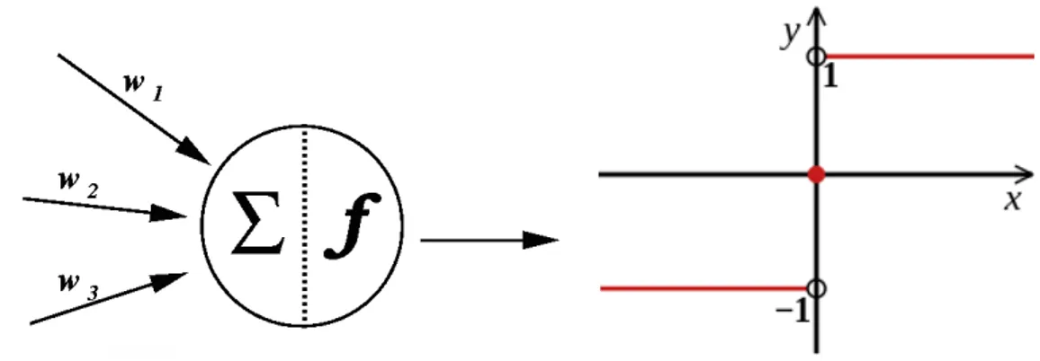
4.2 Activation functions . . . 51
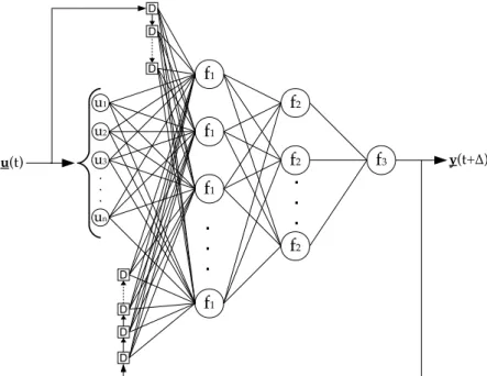
4.3 Feedforward neural networks . . . 53 5
4.6 Learning from errors . . . 60
4.7 Backpropagation algorithm . . . 62
4.8 Stopping criteria . . . 65
4.9 Recurrent neural networks . . . 67
4.10 Real time learning algorithm . . . 69
5 The next generation 75 5.1 Second generation wavelets . . . 76
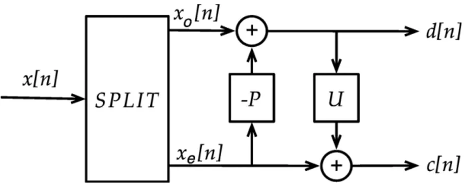
5.2 The lifting schema . . . 77
5.3 A neural network based approach . . . 81
5.4 WRNN based approximators . . . 85
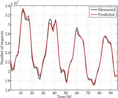
5.5 WRNN based forecast . . . 89
5.6 WRNN based predictors . . . 92
5.7 A P2P model for WRNNs . . . 98
5.8 WRNN-based model enhancements . . . 107
5.9 The next generation of resources . . . 115
6 A2I: Artificial Artificial Intelligence 117 6.1 Amazon’s Mechanical Turk . . . 118
6.2 WRNN based crowdsourcing . . . 120
6.3 WRNN based workflow manager . . . 125
6.4 Companies as humans’ clouds . . . 128
6.5 A lesson from Quantum Electrodynamics . . . 135
6.6 Assisting workflow executions . . . 138
7 Inanimate reasons 139 7.1 Keeping a profile . . . 139
7.2 Social networks dynamics . . . 142
7.3 Paths and distances . . . 144
7.5 The RBPNN classifier . . . 150
7.6 User clustering from RBPNNs . . . 153
7.7 A parallel implementation . . . 156
7.8 Cloud-based strategies . . . 160
7.9 Facebook as a test ground . . . 163
7.10 Comprehensive identities . . . 167
7.11 The inanimate reasoner . . . 171
8 A3I: Artificial A2I 173 8.1 A network of collaborations . . . 174 8.2 RBPNN continuous learning . . . 178 8.3 RBPNN driven workgroups . . . 181 8.4 Smart workflows . . . 184 8.5 Dear Jeff . . . 191 8.6 Artificial3 Intelligence . . . . 193 9 Conclusions 195 Acknowledgements 199 Bibliography 201
CHAPTER
1
Introduction
An architect, a hooker and a programmer were talking: ”Everyone knows mine is the oldest profession,” said the hooker. “But be-fore your profession existed, there was not the divine architect of the universe?” The archi-tect asked. Then the programmer spoke up: “and before an architect, what was there?” “Darkness and chaos,” the hooker said. “And who do you think created chaos?” the pro-grammer said.
Science is a hobby of mine as well as strolling, and such two hobbies do not differ so much after all. Science is the act of walking around concepts, theories, approaches and experiments by continuously getting lost along the paths of thoughts and streams of consciousness. Both such two hobbies of mine can be extremely satisfactory when you finally reach new and unknown places, nevertheless it has been said that the way itself should matter more than the destination, and I agree. As a matter of fact, along the trip that I am called to recap in this thesis, I’ve increasingly found
myself unable to write anything regarding my destination without accounting the path itself. Therefore, in the following pages, I will try to explain the destination of my researches, which is intriguingly contained in the title of this thesis, however not before I have asked for the reader’s kindness in order to be followed along the quite loopy upcoming path. I make a promise though: every bit of information contained in such a path will be shown to be a mandatory piece to build our destination. As for the title of this work I am well aware that every name contains a promise, and my promise is to keep up with a challenge: trying to tackle with the nature itself of human intelligence, trying to model it, manage it, predict it. In the very end, only to ennoble it. Of course, after a fast scroll through the table of contents, it will be obvious that the linchpin of this work is all about crowdsourcing: the nature itself, the involved architecture, the manageability, the possible improvements and the related ethical consequences. The latter are the motif forces that drive the entireness of this work, on the other hand I will briefly discuss about them only at the very end of this thesis. One of the step to undertake to understand this work involves a new conception of crowd and crowd sourcing models, that in a certain portion of this work will be modeled similarly as clouds of some-how-connected brains that, not differently from hardware processors and computational nodes, are concurrently involved on the solution of a set of tasks. The definition is not occasional since also the major crowdsourcing platform, the Amazon’s Mechanical Turk, has been defined by its founder as: an Artificial Artificial Intelligence. Despite that, in this thesis, I would like to improve and exceed the limits of such a definition which, as it will be unveiled, is not only literally disrespectful of the human nature of the Turkers, the back end workers of the Mechanical Turk, but also disagreeable in its profound implications. As for any other scientific work also this thesis is born from a couple of questions: is it possible to do it better? Is it possible to join both the clear advantages of crowdsourcing with a more agreeable consequences for the workers? Is it possible to obtain an automatism of some kind to model and manage such human worker crowds?
Those questions have been asked in a precise moment and in a precise place: the year is 2015, the place is the Lipari isle. The occasion to ask such questions and
11
elaborate on them was given by a fortunate meeting with prof. Michael Bernstein from Stanford University and actual inspirer for the title of this thesis. The conclusions we reached were few but important:
1. Crowdsourcing is based on the certainty of workers availability 2. A skill-based pyramidal structure tampers with the previous point 3. It is paramount then to model availabilities from human behaviors 4. The execution of a crowd-based workflow should become predictable 5. New approaches to crowd modeling and behavior prediction are required Surprisingly, I discovered that the best part of the researches performed during and before my PhD studies, were complying with many of the key points needed for what prof. Bernstein was calling the “crowdsourcing revolution”. At that point the path of this thesis simply unfolded by itself: the milestone where there, the rest was only a matter of connecting them. As said before, the path is what matters. During my studies and my personal growth I had the undeserved fortune to be led on a path crossing disciplines and methods, mixing Physics, Astrophysics, Cosmology, Engi-neering, Energetics, and, finally, Computer Science. This path gave me a personal perspective on chaotic phenomena that I tried to apply at the best of my possibil-ities to the topic of this thesis. The results were as surprising as unexpected, but, eventually, quite interesting. Modeling human beings is not an easy task and I would not have been up to this challenge if I would have only based my approach on my own ab initio assumptions. Instead of that I have tried to let the models emerge by themselves while applying some mathematical methods such as wavelet analysis and several advanced tools such as neural networks.
The developed methodologies and algorithms have been published or submitted to important international journals such as IEEE Transactions on Neural Networks, IEEE Transactions on Industrial Informatics, Neural Systems, Applied Energy, the In-ternational Journal of Mathematics and Computer Sciences, etc. Note that a portion of the mainstream concepts have been based on countless insights received while pre-senting our solutions to conferences such as the IEEE International Joint Conference
on Neural Networks, the International Conference on Artificial Intelligence and Soft Computing and IEEE Symposium Series on Computational Intelligence, for several editions. The help of the scientific community, its constant support, the comments and criticisms received, has been fundamental for the continuation and improvement of the presented research works. A special tribute of gratitude must be anyway rec-ognized to prof. W lodzis law Duch, now deputy Minister for Science and Education in Poland, former head of the Department of Informatics at the Nicolaus Copernicus University, not only an esteemed scientist but also excellent teacher with whom sev-eral times I had the privilege to chat, in front of a cup of tea or sandwiches, and learn the fundamentals of Neural Network and Neurocognitive Informatics directly by one of the main contributors of such fields, vastly known in the scientific community for his computational approach to human mind modeling using Information Theory and Neural Networks.
As I will explain in Chapter 2 the possibility to play with chaos and extrapolate chaotic models take advantages of centuries of meditations and has very long roots. Taking advantage of the gigantic studies already performed by the greatest names of Science I have tried to interpret chaos and find a peculiar order in it starting with Information Theory and Wavelet Analysis. I will give the mathematical basis in Chapter 3. Wavelet analysis permits us to pack the information related to a phe-nomenon into a few numerical coefficients, this is the perfect kind of set you can try to model using neural networks. Of course to let the reader appreciate the advancement proposed in the field of Neural Networks I firstly propose some mathematical basis in Chapter 4, then I will explain in Chapter 5 how I have decided to enhance those tools by means of a personally developed new architecture called Wavelet Recurrent Neural Network, then an extended set of examples and ground tests will be given to the reader. The developed approach, especially when bound to specific mathematical formulations of the problem, among all the other proposed applications, gives us a way to obtain resources availability predictions beforehand in order to preserve the Quality of Service for distributed systems. As it will be shown, this approach has been shown to be extremely useful when applied, in a particular fashion, to workers availability for crowdsourcing projects. In Chapter 6 this thesis will finally enter on
13
the playground of the Mechanical Turk itself while a new conception of Artificial2
Intelligence will be formulated by using Radial Basis Probabilistic Neural Networks as classifiers. The latter will be constituting optimal crowd clustering tools in or-der to unor-derstand, model and predict the behavior of human groups as well as their natural predisposition to connect in social or collaborative networks. The developed approach will be used for the specific purpose of this thesis, in fact in Chapter 7 it will be shown that it is possible to model and create workgroups of people in order to better accomplish a certain task basing on their characteristics, professional skills, experiences, etc. As a matter of fact it will be shown that it is possible to concentrate all those choices, generally made by a company manager, into an Inanimate Rea-soner. Finally, this last frontier of automated company management based on Radial Basis Probabilistic Neural Network will be joined with the said Wavelet Recurrent Neural Networks, also providing an appropriate mathematical model and the related software system in order to model, manage and optimize the execution of complex workflows. Therefore in Chapter 8 the Artificial3 Intelligence will be presented as an overall ensemble of mathematical and technological tools that jointly aims at making the announced “crowdsourcing revolution” possible. Due to the the complexity of the path it seemed reasonable to split it in steps, namely one for each chapter. At the end of each chapter therefore a specific section will try to summarize the meaning and implications of the chapter itself and lead the reader to the following chapter by highlighting the connections and motifs. Finally, in the remaining part of this thesis, and oppositely with respect to this Introduction and, eventually, the final Acknowl-edgments, the use of singular pronouns will be abandoned. In fact, despite of the traditions and rules which compel me to write only my name as author of this thesis, none of the following content would have been possible without the key contribution of a lot of other co-authors which populate part of the bibliography nearing my name. Therefore, from this moment I will use the plural noun “we”, since this is not a one man work but the non-linear superposition of contributions coming from an active collaboration of which I am only a very small part. Enjoy the reading.
CHAPTER
2
Bringing chaos into order
Chaos: When the present determines the fu-ture, but the approximate present does not approximately determine the future.
Edward Norton Lorenz
In 1795, by a decree of the National Convention, a new professor of mathematics was called to join the ´Ecole Normale de Paris. He was named Pierre Simon, marquis de Laplace, but he is now universally known as Laplace. Laplace was also recognized for his so called newtonian fever and he left no occasion to remark his deep beliefs on the deterministic nature of the Universe. Therefore, the words he pronounced during his Course of Probability (reported on A Philosophical Essay on Probabilities, [118] one of his most famous writings) are not surprising: !We may regard the present state of the universe as the effect of its past and the cause of its future. An intellect which at a certain moment would know all forces that set nature in motion, and all positions of all items of which nature is composed, if this intellect were also vast enough to submit these data to analysis, it would embrace in a single formula the movements of the greatest bodies of the universe and those of the tiniest atom; for such an intellect nothing would be uncertain and the future just like the past would be present before its eyes." These are known facts, as well as the invitation that the
same ´Ecole Normale de Paris extended in 1797 for the same position, yet held also by Laplace, to Giuseppe Lodovico Lagrangia, also known as Joseph-Louis Lagrange. Laplace and Lagrange soon established a deep bound of respect and friendship, on the other hand, as Cournot let us know [54], the two mathematicians were also well known for the strength of their verbal fightings. During one of such verbal fights Lagrange pronounced his famous sentence: !I regard as quite useless the reading of large treatises of pure analysis: too large a number of methods pass at once before the eyes. It is in the works of applications that one must study them; one judges their ability there and one apprises the manner of making use of them.". Also the words of Lagrange are not surprising, in fact Marcus Du Sautoy describes him pronouncing similarly strong words [65] during a successive episode. The mentioned episode recalls both Lagrange and Laplace while participating to an high level cultural gala in the Palais du Luxembourg. During this gala a colleague senator, Cauchy his name, while accompanied by his very young son, met the mathematicians. After an interesting talk with the senator’s son, Lagrange gave further use of his strong speaking, addressing the other numerous dignitaries of France, while pointing his fingers to the young boy in a corner: !See that little young man? Well! He will supplant all of us in so far as we are mathematicians", and then addressing his father !Don’t let him touch a mathematical book till he is seventeen [...] if you don’t hasten to give Augustin a solid literary education his tastes will carry him away" [18]. Augustin Louis Cauchy was indeed the name of the boy: “the” Cauchy, father of modern Math. Was Lagrange saying that mathematical education was not important in XIX century? Of course not. Lagrange was well aware that great changes would suddenly reform the basis of mathematics, logics and sciences. The optimistic view of Laplace was in facts definitively doomed: the scientific community was beginning to recognize that, despite the perfection and elegance of pure analysis, it was not sufficient to describe the rounding nature and its phenomena. The scientist, under the newtonian assumption of a deterministic world, were convincing themselves that starting by an approximated knowledge of the initial status of a dynamic system, it would have been possible to determine its temporal evolution. This philosophical assumption was at the very core of XIX century science revolution. Despite of that
2.1. BUILDING CHAOS 17
assumption, in fact, there were increasingly strong evidences of systems that were not describable by the existent analytical laws which, while able to describe the vastness of planetary motion, where completely falling apart when trying to the describe the motion of dust.
2.1
Building chaos
In 1870s finally the word chaos was legitimately admitted in the scientific dictionary thanks to Ludwig Boltzmann and James Clerk Maxwell and their theory of statis-tical thermodynamics. Their molecular chaos assumption postulated that during a two-body collision, between particles in an ideal gas system, there is no correla-tion of velocity. This assumpcorrela-tion allowed us to develop a molecular chaos theory of bodies in gas phase. As a side effect the theory finally introduced the concept of chaotic dynamics. Since that moment the most important scientists contributed to the foundation of chaos theory: from Poincar´e to Hadamard, from Lorenz to Kol-mogorov. The latter, Andre¨ı Nicola¨ıevitch Kolmogorov, can be surely considered the legitimate father of modern chaos theory due to his revision of the theories yet de-veloped by Poincar´e [112]. Kolmogorov demonstrated that a quasiperiodic regular motion can persist in an integrable system even when a slight perturbation is intro-duced. This statement is also know as the KAM theorem due to the initials of the authors, Kolmogorov, Arnold and Moser, who independently reached the same con-clusions [112, 140, 197]. While the intentions of the authors were to indicate the limits to the integrability of map functions, this theorem also gives the basis to understand the transition of a stationary deterministic system into a chaotic state. As a matter of fact in an integrable system all the possible status transitions are regularly quasi periodic and introducing a neglectable perturbation with respect to the system, the quasi periodic properties are not affected. On the other hand, as shown by the KAM theorem, if we consider an increasingly strong perturbation, the probability to affect the quasi periodicity of the system increases until chaotic trajectories are developed and a totally chaotic status is reached. In this latter stage the constants of motion are not preserved excepted the total energy, for this reason the consequences of the KAM
theorem are also generally called ergodic principle. Despite its apparent strangeness with respect to the topic of this thesis, the ergodic principle gives us the very deep meaning of this work when applied to complex systems. In a system describable by means of linear equations, an effect is simply a sum of a certain number of causes in a totally deterministic fashion, accordingly to the principle of causality postulated by Ren´e Descartes. On the other hand, such equations are rarely found to be accurate when trying to describe a natural phenomenon in detail due to its intrinsic discontin-uous or non stationary nature. The latter requires more complex models using non linear solutions in order to reach an accurate enough description of the physical laws. Unfortunately, the non linearity of such systems makes it impossible to preserve the causality principle as described by Descartes since the effect of a small interaction is not anymore accountable by such mathematical models. Non linear models, as developed in the XIX century, were often not robust enough with respect to small interactions, therefore small variations of the initial conditions can lead them to non deterministic states.
2.2
Chasing butterflies
While the KAM theorem and the ergodic principle gave the basis to understand chaos, also due to the works of their predecessors, the official discoverer of chaos is consid-ered Edward Norton Lorenz with his work on deterministic nonperiodic flow [124]. Ironically, the bases of his theory were discovered by chance in 1961 while playing with different approximations with the aim to produce accurate weather forecast with a quite primitive computer. It is reported in literature [86] the famous episode of Lorenz obtaining different solutions to his algorithm basing on the different ap-proximations (3 or 6 decimal digits). The problem, discovered Lorenz, was not the approximation capabilities of the machine, but the non linear nature of the system that, due to small multiplication errors at each iteration, was suffering of an in-duced exponentially divergent trajectory in the state space. In 1972, Philip Merilees, chairman of the International Conference of the Association for the Advancement of Science, invited Lorenz to present his work, but was Merilees itself to decide the
2.3. CHAOTIC INFLUENCES 19
title. The paper was entitled “Predictability: Does the Flap of a Butterfly’s wings in Brazil Set off a Tornado in Texas?” [123], it contained the formulation of what is commonly called the butterfly effect. Finally, in 1975, Edward Norton Lorenz produced the results of a computer simulation graphically describing the divergence effect caused by approximation, and suddenly he understood that the simulations should have been reversible. The consequent results contributed to another discov-ery: the Lorenz’s attractors. These attractors were immediately defined by Lorenz itself “strange attractors” due to their shape and evolution in double spirals like the wings of a butterfly. The comprehensive theory including Lorenz’s discoveries will then be called with the name of Chaos Theory by James A. Yorke [120]. Yorke will say that Lorenz’s attractor was capable to devise the intrinsic structure and the sta-bility of systems that apparently show no stasta-bility or structure. On the other hand no one was yet aware of the real capabilities offered by the newborn theory.
2.3
Chaotic influences
As shown by Yorke, Lorenz, Packard, Mandelbrot, and many others it was possible to devise structures, recurrences and mathematical properties from a multitude of apparently indeterministic phenomena. Chaos theory was shedding light on a new interpretation of nature’s complexity: a natural order describing the interaction of forces and evolution of states that, despite of the intrinsic complexity of such phe-nomena, could be defined by fairly simple solutions. In such an interpretation a stationary phenomena is nothing more than a stable and totally deterministic sys-tem, therefore predictable, where even a small interaction can lead to non determin-istic states, therefore a non predictable behavior. The key factor for such a kind of systems is the minimum amplitude that a small interaction should have in order to break the linearity of the system. The first to take into account such a question was Henry B´ernard in 1901 while studying the water movements when exposed to an heat source: he discovered that, while heating the water, it exists a critical tem-perature after which the water begins to move in small vertical independent cells of fluid. Unfortunately B´ernard, while responsible of describing the phenomenon, was
not able to explain it, in fact an explanation was firstly given after sixteen years by John William Strutt, baron of Rayleigh, that we universally know as Lord Rayleigh. It must be said that the given explanation was technically wrong since Rayleigh was basing its interpretation on slightly different conditions, on the other hand the baron had caught the general reasons at the basis of the phenomenon: during its heating process, the water undergos a reckless battle between viscosity and heat. The first is responsible of maintaining the original uniformity of status and no coherent motion, the second is responsible of breaking the original status introducing a collection of states in uniform motion. Rayleigh understood that such dynamic systems are gen-erally lead by two kinds of forces concurrently trying to impose a configuration by eliminating the other one. Therefore it exists a minimum perturbation amplitude af-ter which the new forces are capable to win the inertia of the system, driving it away from its original configuration and letting its steady and uniform status to undergo a chaotic transition. Fortunately chaos theory can provide us the mathematical tools to build a perturbative model. On the other hand, while it is possible to use chaos theory to model such physical phenomena, is it possible to use the same approach for far more complex system such as a social system? The field of social systems involves far more complex phenomena with respect to any other system. Certainly, as the history of Internet and communication networks shows, social systems do not share the same geometrical properties and spatial symmetries of a pot of water on the fire. On the other hand, such a very complex social system manifests a different kind of order of its own, a set of symmetries that must be extrapolated and that are not evident at a first sight. B´ernard experiment shows that a chaos can emerge from order, but, as Rayleigh has proven, also from chaos a peculiar kind of order can emerge, but only after a chaotic transition. In order to understand a social sys-tem then, it is paramount to understand its chaotic transitions. As Mark Buchanan suggests [32], a typical example of chaotic transition is the explosion of a riot: two man have a fight into a bar, someone else get involved, and so on, until the bar is on fire as well as neighboring shops and hundreds of policemen are fighting against hundreds of hooligans for several weeks (Bradford, April 2001). Despite the cultural and psychological interpretations of the single phenomenon, the answer should be
2.4. A SMALL WORLD 21
searched elsewhere. In 1978 Mark Granovetter, working with Christopher Winship, Douglas Danfort and Bob Philips, mathematically demonstrated that models of col-lective behavior are developed for situations where actors have alternatives and the cost or the benefits of each depend on how many other actors choose which alternative [88]. The key concept is that it exists a threshold for the number of actors choosing the same alternative, this threshold acts as a transition point from the steady equi-librium status to a chaotic evolution until a new status is reached. This threshold is of course different for each individual, on the other hand it is also susceptible of the influences of the collective in which the individual is integrated. Granovetter also demonstrates that a small variation on such an individual threshold for one of the actors can have a profound influence on the entire group. Such influences have been proven to be both hierarchical and iterative processes. The first property results more evident in the social context of companies or working environments, the second in groups of people with common interests. In the year 2000 Malcom Gladwell proved [85] that viral content gets amplified from an individual to another creating a series of iterations and reaching out to the masses. In other words it is possible to build maps of influence starting from a main influencer and building hierarchical or interest based relationships to his second grade influencers and so on. It means that chaotic transitions in social systems are started by influences mappable in peculiar kinds of networks: the small world or scale free networks.
2.4
A small world
In 1998 an article appears in the international journal Nature showing a simple net-work model that can be tuned to introduce increasing amounts of disorder showing that such systems can be highly clustered while preserving a small characteristic path lengths like random graphs [199]. The authors of the article are Duncan Watts and Steven Strogatz, and they call those systems small world networks, by analogy with the small-world [135] phenomenon (popularly known as six degrees of separation). The neural network of the worm Caenorhabditis elegans, the power grid of the west-ern United States, and the collaboration graph of film actors are shown in the article
to be small-world networks. Such networks are represented by the authors as mathe-matical graph where very few nodes are neighboring each others, while in few hops it is possible to reach any destination node starting from any other node. In this kind of networks the distances in terms of numb of hops δpn0, n1q among two nodes n0 and
n1 is generally proportional to the logarithm of the size of the network itself, defined
as the number of nodes N, therefore
δpn0, n1q9 log N (2.1)
This so called small world effect is particularly noticeable in many social contests such as social networks, collaborative networks, companies and workgroups. The underlying structure of the Internet itself shows to be a fairly evident small world network. Successively, in 2002, Reuven Cohen and Shlomo Havlin have shown that some yet known small world networks, in particular, shares a peculiar property: their degree distribution follows a power law, at least asymptotically [52]. In other words, in such particular networks, considering the nodes retaining a number k of connections as a fraction P pkq of the total number of nodes in the network, this fraction P pkq typically [43] scales as a power law
P pkq9k´γ (2.2)
where generally γ P r2, 3s Ă R. Cohen and Havlin have also shown that the average distance between nodes in scale free networks is much smaller than that in regu-lar random networks. Moreover, their studies on percolation in scale free networks demonstrates that while a chaotic transition generally occurs only in the limit of extreme dilution, several nodes are often critical to determine the evolution of the en-tire network. Finally, in [51] Cohen and Havlin demonstrate that scale free networks are ultra-small worlds. Speaking of a whole network in its entirety, in a small-world network if we define a diameter d as
d “ max
n0,n1PV tδpn0
2.4. A SMALL WORLD 23
where V represents the set of nodes composing the network, then, due to (2.1), it immediately follows that
d9 log N (2.4)
On the other hand, as the authors demonstrated, scale free networks within the constraint γ P r2, 3s ĂR have a much smaller diameter with
d9 log log N (2.5)
While the derivation is valid for uncorrelated networks, the authors also detail that for assortative networks the diameter is expected to be even smaller. This latter kind of networks was described by Newman in [160] where he gives the definition of assortative network as a network where the nodes that have many connections tend to be connected to other nodes with many connections. Newman also finds that social networks are mostly assortatively, while technological and biological networks that tend to be disassortative, moreover he finds that assortative networks percolate more easily being also more robust to vertex removal. These considerations paint a unique picture: social networks are stable and resilient and therefore prone to spread influences among nodes, whether we are talking of diseases in a city, information in an online social network, interactions among workers of a company, or influences among users or maintainers of a service. Influence spreading on a social network have therefore peculiar patterns that guarantee the outcome. A question remains: is it possible to model such patterns and then predict the behavioral evolution of a social network over time? Again a bit of chaos theory, and in particular the ergodic principle, should be taken into account. If, in fact, as said before, chaotic transitions in social system are started by influences, and given that such influences resulted mappable as scale free networks, it seems legitimate to ask if it is possible to study social networks in terms of chaotic transitions. In this latter scenario two elements must be defined: the influences leading to such transitions, and a critical threshold driving the system. From this point the next step is obvious, since there exists only one considerable kind of influences flowing uninterruptedly in a social network: information. As a matter of fact, it has been proven many times that information dynamic does not
differ from epidemic dynamic and that there is no difference between the spreading of a pathogen or the diffusion of an idea, the models are similar, both of them non linear, both of them chaotic, both of them ergodic. But in order to define things such as transitions, thresholds and system energy, it is imperative to quantify by means of a measurement. It is then imperative to measure information.
2.5
All form is formless
While trying to analyze social networks in terms of information flows is an inevitable starting point, it is also a comforting arrival point that closes the circle of chaos theory. As a matter of fact, it would be impossible to understand any aspect of chaos theory without considering its interpretation under the lights of information theory. This latter, on the other hand, is based on a primitive concept: information. Due to the primitivity of this concept, it is quite difficult to give an appropriate definition of information. Generally speaking, in order to measure information, it would seem necessary to give an a priori definition of the form in which information is retained. Fortunately, whether or not information and its form can be properly defined, information can certainly be measured and algebraically represented. As well as Lorenz can be considered the legitimate author of Chaos Theory, the same role, relatively to Information Theory, should be assigned to Claude Elwood Shannon, but without forgetting that his work has been based on the previous studies of Gibbs, Boltzmann and a lot of other predecessors. Shannon’s work [183] explains that there is no real need to know the form as far as it is possible to define a proper mathematical domain describing the information flow. The Shakespeare’s character of Cardinal Pandulph would say that !all form is formless, order orderless", as he does in the third act of King John, unwillingly giving us a perfect definition of information: a structure-less structure. If it is in fact impossible to obtain an a priori definition of information, on the other hand it is quite easy to measure it once its mathematical definition has been given. Shannon’s work not only gives that, but he also assigns a prediction probability, nowadays known as Shannon’s entropy, in order to universally define the information content. In particular, given a content carrying information,
2.5. ALL FORM IS FORMLESS 25
and known a certain portion of such a content, we could want to immagine the rest of the message. If we assign a probability pi to each possible outcome, we can measure
the information carried by that outcome as H “ ´ÿ
i
pilog2pi (2.6)
The consequence is quite obvious as its interpretation: if we are able to completely determine with total certainty the outcome without having seen it, then its infor-mation content is zero [184]. As a matter of fact, we have no new inforinfor-mation after the outcome becomes known, and, from this point of view, this kind of information measures tell us how much unexpected is an outcome. Therefore it is the quantity of information characterizing our a priori knowledge that affects the quantity of in-formation we can get from the outcome. Certainly this aspect of Shannon’s entropy should affect also our mathematically exact analytical models, as well as any other reproducible algorithm. As a matter of facts, given detailed enough initial conditions, a mathematical model is able to predict one and only one result with an outcoming probability of 1. Shannon’s interpretation of such a model is simple and terrible: the model predicts nothing. In facts no information is predicted by an analytical model, due to its certainty, therefore all the information must be contained in the initial data. It is only well hidden. Then, if wherever it is possible to formulate a working mathematical set of laws and conditions capable to predict the future outcome of a phenomena starting by a data set of initial conditions and boundary conditions, it means that all the information is contained in such a data set, the next question can be only one. Where is such information hidden? The reason to bind wavelet analysis with neural networks is contained in the last question as well as in this chapter. While the historical importance of chaotic models has been shown, we hereby propose a new methodology to cope with non linear phenomena without imposing any constraint or mathematical model ab initio. Wavelet analysis will permit us to obtain a different representation of the data. Such a representation will be more suitable for neural networks which will be used to cope with chaotic systems due to their robustness to noise and misleading data. By binding the said two approaches it will be shown that
it is possible to model the chaotic behavior of non linear systems, then allowing us to tackle with the nature itself of human behavior in terms of chaotic transitions and information measurements. The purpose is to let the models be born from the ex-perimental data themselves making no unjustified assumption. This will be possible only thanks to the high versatility of the used mathematical and computational tools as well as their yet proven suitability for chaotic models.
CHAPTER
3
Bringing order into chaos
Chaos was the law of nature. Order was the dream of man.
Henry Adams
The wavelet analysis give us a powerful tool to achieve major improvements on information-based representation of data especially when such data are affected by an apparently chaotic behavior. In general wavelet decomposition is used to extract a shortened number of non-zero coefficients from a signal representative of the phe-nomenon. In this manner the wavelet analysis can be used in order to reduce the data redundancies so obtaining representation which can express their intrinsic structure. The main advantage of the wavelet use is the ability to pack the energy of a signal, and in turn the relevant carried informations, in few significant uncoupled coefficients. In particular the performance of the wavelet decomposition can be noticed for non-linear dynamical systems and predictors [57]. The wavelet transform, in fact, packs the energy of a signal reducing the redundancies and showing the intrinsic structure in time and frequencies. The so obtained representation with wavelet decomposition offer advantages while used with neural networks, as will be introduced in the next chapters. For now we will give a general description of the mathematical support.
3.1
Wavelet theory
A general isomorphic linear application on a metric field, e.g. R, which is able to describe a signal as a series expansion of waveforms, e.g. the Fourier expansion, is called linear time-frequency transform. The waveforms involved in such a transform are called time-frequency kernels and can be used as basis elements of an Hilbert space. Considering a signal represented by a function f :R Ñ R, and f P L2
pRq, it is possible to define a transform as a bijection T : L2pRq Ñ L2pRq so that
#
T rf ptqs “ ξptq T´1
rξptqs “ f ptq (3.1)
where T´1 : L2pRq Ñ L2pRq represents the inverse transform.
In order to understand the (3.1) it is necessary to recall few elements of algebraic and functional analysis. Let Sn be a n-dimensional a linear space, therefore a set of
n linearly independent elements txkP Snunk“1 form a basis for that space. Moreover,
since Snis a finite-dimensional linear space, it can be equipped with an inner product.
Such a product allow us to obtain an orthonormal basis of Sn from any other basis using the Gram-Schmidt process [187]. Finally any basis tvk P Snunk“1 for S
n is the
image under an invertible linear transformation of an orthonormal basis of Sn. In a
more extensive scenario, taking into account also infinite-dimensional spaces, let SH
be an Hilbert space, or, in other words, let SH be an abstract vector space possessing
the structure of an inner product that allows lengths and angles to be measured and that, consequently, is also a complete metric space with respect to the distance function induced by the inner product [14].Under the said conditions, a collection of vectors txk P SHukPZ is a Riesz basis for SH if it is the image of an orthonormal
basis for SH under an invertible linear transformation. In other words, if there is an
orthonormal basis tekukPZ for SH and an invertible transformation M such that
M ek “ xk @ k PZ (3.2)
3.1. WAVELET THEORY 29
t˜xj P SHujPZsuch that xxk|˜xjy “ δkj, where δkj is the Kronecker delta. Such collection
t˜xj P SHujPZ is called biorthogonal basis with respect to txk P SHukPZ for SH, and it
is also a Riesz basis of SH. If txk P SHukPZ and t˜xk P SHukjPZ are Riesz basis forSH
then there are non-negative constants α and β with α ď β such that @ x P SH ñ α||x||2 ď ÿ kPZ |xx|xky|2 ď β||x||2 @ x P SH ñ α||x||2 ď ÿ jPZ |xx|˜xjy|2 ď β||x||2 (3.3)
The (3.3) si also called Cauchy-Schwarz frame inequality for Hilbert spaces [44]. It is important to highlight that if txk P SHukPZ and t˜xk P SHukPZ are orthonormal basis
then the biorthogonality condition is obvius (e.g. taking ˜xk “ xk) and the (3.3) is
trivially verified by means of the Plancherels formula with α “ β “ 1. In fact if txk P SHukPZ and t˜xk P SHukPZ satisfies the frame inequality with α “ β “ 1 and
if |xk| “ |˜xk| “ 1 @ k P Z, then txk P SHukPZ and t˜xk P SHukPZ are biorthonormal
basis for SH. A different way to characterize some of these properties is to think of
two operators T and T´1 associated to the Riesz basis tx
k P SHukPZ. The first can
be called analysis operator T : SH Ñ L2 given by T pxq “ txx|xkyukPZ; the second
can be called synthesis operator T´1 : L2
pRq Ñ SH given by T´1pT pxqq “ x. In
this formalism, txk P SHukPZ is a Riesz basis if and only if T is a bounded linear
bijection from SH onto L2, but then it follows that SH “ L2pRq. It follows then it
is possible to define a transform as a bijection T : L2
pRq Ñ L2pRq so that, given a signal f : L2 pRq Ñ L2pRq, # T rf ptqs “ ξptq T´1 rξptqs “ f ptq
where T´1 : L2pRq Ñ L2pRq represents the inverse transform, coming back to the
(3.1).
Consider now a complete generator set for L2pRq and let the elements of such a set be time-frequency kernels tφγuγPΓ where φ represents a multi parametric function
of index γ and Γ is the indexing frame. Moreover let it be φγ P L2pRq with ||φγ|| “ 1
time-frequency transform Tγ : L2pRq Ñ L2pRq as Tγrf ptqs “ xf |φγy “ `8 ż ´8 f ptqφ˚ γptqdt (3.4)
For such a transform, thanks to the Parseval theorem it is possible to demonstrate that Tγrf ptqs “ `8 ż ´8 f ptqφ˚ γptqdt “ 1 2π `8 ż ´8 f pωqφ˚ γpωqdω (3.5)
Then it is possible to decompose the signal function f into a continuous superposition of γ-intervals both in the time domain and in the frequency domain. Therefore if the value of φptq is near to zero for any t in a small interval around a certain value tu, then
xf ptq|φγy will depend only from the value of f ptq on the selected interval. Analogously
if φγpωq is near to zero for any ω in a small interval around a certain frequency ωu,
then the second member of the (3.4) proofs that xf pωq|φγy reveals the properties of
f pωq around ωu. The two properties yet explained have tremendous consequences for
the field of signal analysis since, due to this theorem, it is possible to construct a short time Fouriers transform by means of a small subdomain g, called shifting window, and then translate it by a shift tu and modulating it by a frequency ωu so that
φγptq “ gωutuptq “ e
iωutugpt ´ t
uq (3.6)
Similarly, it is possible to construct a wavelet kernel by means of a scaling factor s and a shifting factor tu starting from a motherwavelet function ψ :: L2pRq Ñ L2pRq
so that φγptq “ gstuptq “ 1 ? sψ ˆ t ´ tu s ˙ (3.7) This latter is also called time-frequency scaling and shift relation. By using the wavelet kernels defined in (3.7) it is then possible to transform the space L2pRq by means of a complete Rietz basis tφγuγPΓ by varying on a specific set of scaling and
shift parameters for each φγ. The main advantage of such a decomposition is the
3.1. WAVELET THEORY 31
the signal amplitude is distributed. In this manner it is possible to associate to each signal in L2ppRq an unique energy distribution known as time-frequency signature of the signal in the wavelet domain. Such a signature it is often more useful with respect to the classical spectrum resulting from a Fourier transform (continuous or discrete), since this latter only decompose a signal in limited frequency bands. By using a time-frequency representation such as the wavelet decomposition a greater number of information can be carried. It is finally possible to reconstruct the original in-formation with the time-frequency product xf |φγy represented on the time-frequency
plan tpt, ωqu ĂR2 as a geometrical region. The position and surface of such a region depend by the time-frequency spread of the kernel φγ and therefore are mainly
de-termined by the wavelet scaling factor s and shift factor tu. One of the properties of
a motherwavelet is the unitary norm, therefore
||φγptq||2 “ `8
ż
´8
|φγ|2dt “ 1 (3.8)
It this the possible to cope with |φγptq|2 as with a probability distribution centered
on a point tuγ defined as
tuγ “ `8
ż
´8
t|φγ|2dt (3.9)
following this mental schema interpreting |φγptq|2 as a probability distribution, it is
also possible to define a standard deviation and consequently to obtain the definition of a variance σ2tupγq “ `8 ż ´8 pt ´ tuγq2|φγptq|2dt (3.10)
It is then possible to recognize σ2
tupγq as the time-frequency spread of the kernel φγ
it is possible also to prove σt2upγq “ `8 ż ´8 |φγ|2dω “ 2π||φγ||2 (3.11)
It is then possible to represent an equivalent of (3.9) on the frequency domain. This point is the central frequency of φγ and is defined as
ωuγ “ 1 2π `8 ż ´8 ω|φγpωq|2dω (3.12)
similarly it is possible to represent the time-frequency spread also on the frequency domain as σω2upγq “ `8 ż ´8 pω ´ ωuγq2|φγpωq|2dω (3.13)
It is now clear how important is the time-frequency spread associated with a certain wavelet decomposition starting from the chosen wavelet kernels tφγu: such a spread
determines the resolution in time and frequency of each wavelet kernel. Basing of such resolution the wavelet transform is able to devise the time-frequency signature of a signal by characterizing the energy distribution for each one of the different time and frequency resolutions resulting from the wavelet kernels. For a given time-frequency plan tpt, ωq P R2u, each wavelet kernel φ
γ selects a region Ωγ Ă tpt, ωq P R2u called
Heisemberg box and defined as
Ωγ “ „ tuγ´ σt2pγq 2 , tuγ ` σt2pγq 2 ˆ „ ωuγ ´ σω2pγq 2 , ωuγ` σω2pγq 2 ĂR2 (3.14)
Finally it is possible to prove [200] the existence of a minimum for such a region and, due to the (3.8) it results [128] a typical Heisemberg’s formula
surfpΩγq “ σt2pγqσ 2 ωpγq ě
1
2 (3.15)
3.2. WAVELET TRANSFORM 33
follows that, differently with respect to the Fourier transform, it is not possible to obtain a point to point bijective correlation between a signal and its wavelet transform since the time-frequency signature of such a signal is not concentrated in a point but results from the superposition of different scales (therefore a different scaling factors) at different time and frequencies (different values of tu and ωu) at different
time-frequency resolutions. In an over-simplified example, let suppose that for a pair ptu, ωuq P tpt, ωqu Ă R2 we use an unique wavelet kernel φγptu,ωuq centered in
ptu, ωuq, then it is possible to obtain the related time-frequency resolution Ωγptu,ωuq.
The obtained Ωγptu,ωuq is a rectangular neighborhood of ptu, ωuq where it is possible to
locate a portion of the energy of the signal f as
ε“fpΩγptu,ωuqq ‰ “ˇˇxf |φγ ptu,ωuqy ˇ ˇ 2 “ ˇ ˇ ˇ ˇ ˇ ˇ `8 ż ´8 f ptqφ˚ γptu,ωuqptqdt ˇ ˇ ˇ ˇ ˇ ˇ 2 (3.16)
3.2
Wavelet transform
As devised in the previous section, transforming the L2pRq space by using a Rietz basis of time-frequency kernels allow us to let different properties of a signal emerge in the time-frequency plan. Since different signals can be characterized by very different properties both in time and frequency domains, it is therefore agreeable that a lot of different time-frequency kernels basis can be used and customized in order to analyze specific kinds or families of signals. A quite sizable group of time-frequency decom-positions constitutes the wavelet transform family. A wavelet transform decomposes a signal transforming the space with a specific basis computed starting by a common motherwavelet function properly shifted and scaled. Specifically we call wavelet a linear function ψ : L2
pRq Ñ L2pR quadratically summable and with zero average and belonging to a class of γ-neighborhoods centered on a point tu “ 0. Then it follows
that
`8
ż
´8
`8
ż
´8
|ψptq|2dt “ 1 (3.18)
While the latter is the normalization condition ||ψ|| “ 1, due to the said properties, as in (3.7), it is possible to obtain the time-frequency scaling and shift relations
ψtusptq “ 1 ? sψ ˆ t ´ tu s ˙ (3.19)
Moreover for each resulting kernel the normalization condition must be preserved so that ||ψtus|| “ `8 ż ´8 |ψtusptq| 2 dt “ 1 @ tu, s (3.20)
If the enlisted conditions are verified, given a signal f P L2R, a shift factor t
u and a
scaling factor s, it is possible to define the wavelet transform centered on tu at a scale
s as the functional application Wstu : L
2R Ñ L2R so that Wsturf s “ `8 ż ´8 f ptqψ˚ tusptqdt “ `8 ż ´8 f ptq?1 sψ ˚ˆ t ´ tu s ˙ dt (3.21)
From (3.21) follows the wavelet convolution rule # Wsturf s “ xf |ψtusy “ f ‹ ˜ψsptuq ˜ ψsptuq “ ?1sψ˚ `´t s ˘ (3.22)
Changing to the frequencies domain it is possible to transform ˜ψsptq obtaining its
Fourier transform ˆ F r ˜ψsptqs “ ˜ψspωq “ ? sψ˚ psωq (3.23) Since due to (3.17) it is ψpωqˇˇ ω“0 “ `8 ż ´8 f ptqψptqdt “ 0 (3.24)
3.3. WAVELET FILTERS AND PROJECTORS 35
starting from (3.23) it is possible to demonstrate that ψpωq act trivially as a band-pass filer on the signal f . Therefore computing the convolution f ‹ ˜ψsptuq of (3.22)
we obtain a wavelet scale transform as a band-pass filter on f properly scaled and shifted by means of the factors s and tu.
3.3
Wavelet filters and projectors
Since the wavelet transform, once selected a scale factor s and a shift factor tu , acts
as band-pass filters it is natural to associate the overall wavelet transform to a filter banks varying the parameters s and tu. Let Ψ a set of dyadic wavelet kernels
Ψ “ # ψjn O ψjnptq “ 1 ? 2jψ ˆ t ´ 2jn 2j ˙+ j,nPZ (3.25)
it is possible to show that Ψ is an orthogonal basis of L2pRq, and then that f ptq “ÿ j,n xf ptq|ψjnyψjnptq “ ÿ j,n djnptqψjnptq @ f P L2pRq (3.26)
where djn “ xf ptq|ψjny are called wavelet coefficients. The (3.26) is the practical
link among the wavelet functions and the classical functional analysis based on the Fourier transform. The wavelet family Ψ is called biorthogonal wavelet family and is composed by kernels ψjn that are computed starting by the same motherwavelet
ψ “ ψ00 by using a scaling factor 2j and a shift factor 2jn. In this manner each
one of the wavelet kernels ψjn identifies a portion of the information carried by the
signal on the band with resolution 2j. Using a truncated approximation of (3.26)
it is then possible to obtain a multi-resolution approximation of the signal since the wavelet kernels act in this case as ideal conjugate mirror filters, and in this case the overall decomposition resembles a multi-rate filter bank. Taking advantage of such similarities, the wavelet transform can be easily implemented as filter banks and therefore lowering the computational complexity of the operation. For a discrete signal composed by N samples then the computational complexity is in the order of
OpNq operations. For discrete signals then is possible to construct orthogonal wavelet basis with compact support by means of unidimensional filters. In this manner the construction of a wavelet basis is reduced to the resolution of a multi resolution approximation problem for a signal. Let f P L2pRq be a signal, then the expansion
(3.26) can be interpreted as the difference of an approximations of the signal with resolution 2´j`1 with respect to another approximations of the signal with resolution
2´j. The multi resolution decomposition of a signal represents the signal itself by
means of its projection of a set of orthogonal spaces tVjujPZ. Such projection are
performed by means of the devised filters which acts as a orthogonal projectors on for the orthogonal spaces. The multi resolution analysis of a signal allows us to highlight some characteristics of the signal itself by means of the time-energy signature even when such characteristics are hidden because of interferences, noise or aberrations of the signal, since those interferences generally presents different signatures. The approximation of a signal f at a resolution 2´j is performed by means of a grid o
samples and the related local means on a dimension proportional to 2j. Formally it is possible to define the approximation of a function f P L2pRq at a resolution of 2´j
as the orthogonal projection of f on the space Vj Ă L2pRq. Moreover, in the space
Vj are contained all the possible approximation of f at resolution 2´j. It follows that
@ f P L2pRq D ! fνj “ PVνjrf s M fνj P Vj Ă L2pRq ) ν @ j PZ (3.27)
therefore by fixing a general approximation basis for L2
pRq, the orthogonal projection of f in Vj results to be the function fj P L2pRq so that ||f ´ fj|| is minimal. Then it
follows the definition of Mallat [127] and Meyer [134] of multiresolution. A set tVjujPZ
3.3. WAVELET FILTERS AND PROJECTORS 37 verified Vj`1ĂVj @ j PZ f ptq PVj ô f pt{2q PVj`1 @ j PZ f ptq PVj ô f pt ´ 2jkq PVj @ j, k PZ lim jÑ`8Vj “ č jPZ Vj “ t0u lim jÑ´8Vj “ ď jPZ Vj “ L2pRq (3.28)
then it is possible to state that it exists a set of motherwavelets tΦpt ´ nqunPZ which
is a Rietz basis for V0. Intuitively it follows that Vj is invariant for any translation
proportional to the scale factor 2j. As a result of such properties, a sequence thku
exists such that the scaling function satisfies a refinement equation ϕpxq “ 2ÿ
k
hkϕp2x ´ lq (3.29)
The set of functions tϕj,lpxq|l PZu with
ϕj,lpxq “
?
2jϕp2jx ´ lq (3.30)
is a Riesz basis of Vj. Define now Wj as a complementary space of Vj in Vj`1 , such
that Vj`1 “ Vj‘ Wj, vp2xq P Wj`1, and vpxq P W0 ô vpx ` 1q P W0. Consequently `8
à
j“´8
Wj “ L2pRq (3.31)
A function φpxq is a wavelet if the set of functions tϕpx ´ lq|l PZu is a Riesz basis of W0 and also meets the following two conditions:
`8
ż
´8
and }ψpxq}2 “ `8 ż ´8 ψpxqψ˚ pxqdx “ 1 (3.33)
If the wavelet is also an element of V0, a sequence tgku exists such that
ψpxq “ 2ÿ
k
gkϕp2x ´ lq (3.34)
The set of functions tϕj,lpxq|l P Zu is now a Riesz basis of L2pRq. The coefficients in
the expansion of a function in the wavelet basis are given by the inner product with dual wavelet ˜ψj,lpxq “ ? 2jψp2˜ jx ´ lq such that f pxq “ÿ j,l xf, rψj,ly ψj,lpxq (3.35)
Likewise, a projection on Vj is given by
Pjf pxq “ ÿ l xf,ϕrj,ly ϕj,lpxq (3.36) where ˜ϕj,lpxq “ ?
2jψp2˜ jx ´ lq are the dual scaling functions. The dual functions have
to satisfy the biorthogonality conditions
xϕj,l,ϕrj,l1y “ δl´l1 (3.37)
and
xψj,l, rψj1,l1y “ δj´j1δl´l1 (3.38)
They satisfy refinement relations similar to (3.29) and (3.34) involving sequences t˜hku and t˜gku. In case the basis functions coincide with their duals, the basis is
orthogonal. As shown by Cybenko [56], given a continuous function f : R Ñ R it exist a discriminating function σ so that is possible to obtain a representation
f pxq “
8
ÿ
i“1
3.4. CONJUGATE WAVELET MIRROR FILTERS 39
where wi, bi P R and ai PRn is a n-dimensional real vector. If σ is dense in r0, 1sn it
follows that any continuous function f can be approximated by a finite sum. Analo-gously according to wavelet theory we can state that
f pxq “ 8 ÿ i“1 widetpD 1{2 i qψpdix ´ tiq (3.40)
is dense in the L2pRnq. We will call tdiudilatation vector and ti translation vector,
while will be Di “ diagpdiq and ψ will be called mother wavelet function whose
translates and dilates forms the basis for the L2pRnq space [176]. In this scenario,
as a matter of facts, the space Vj can be interpreted as a topological grid of cells
of dimension 2j characterizing a resolution of 2´j. From the (3.28) also follows that
given an approximation with a resolution 2´j it contains all the information in order
to compute a further approximation with a resolution 2´j´1. By iterating the process
the resolution of course will be reduced of a factor of 2 for each iteration, therefore, approaching 0, all the information details will be lost since
lim
jÑ´8||fj|| “ 0 (3.41)
On the other hand, if we immagine on the opposite to make the resolution diverge to `8 it obviously follows that the approximation should converge to the original signal itself and that
lim
jÑ`8||fj ´ f || “ 0 (3.42)
where the norm ||fj ´ f || is indeed the approximation error.
3.4
Conjugate wavelet mirror filters
As explained in the previous section, it is possible to generate an orthogonal basis for each Vj starting from a scaling function Φ. Each one of the generated function
function Φ generating an orthonormal basis for V0 it is possible to obtain it using 1 ? 2Φ ˆ t 2 ˙ PV1 ĂV0 (3.43)
and since tΦpt ´ nqunPZ is an orthonormal basis for V0 it is possible to decompose it
as the expansion 1 ? 2Φ ˆ t 2 ˙ “ ÿ nPZ hrnsΦpt ´ nq (3.44)
where h[n] represents the discrete conjugate filter
hrns “ A 1 ? 2Φ ˆ t 2 ˙ ˇ ˇ ˇΦpt ´ nq E (3.45)
Applying the Fourier transform to the members of the (3.44) it follows that $ ’ ’ ’ & ’ ’ ’ % Φp2ωq “ ?1 2hrωsΦpωq hrωs “ ř nPZ hrnseinω (3.46)
At this point it is useful to represent Φrωs as direct product of hrωs so that Φp21´pωq “ ?1
2hr2
´pωsΦp2´pωq
@ p ě 0 (3.47)
and then by substitution and truncation to the P ´ th factor it is possible to obtain
Φpωq « ˜ P ź p“1 hr2´pωs ? 2 ¸ Φp2´Pωq (3.48)
If Φpωq is continuous in 0 then lim
P Ñ`8Φp2 ´Pωq “ Φp0q, and therefore Φpωq “ ˜ `8 ź p“1 hr2´pωs ? 2 ¸ Φp0q (3.49)
3.5. ORTHOGONAL WAVELET BASIS 41
Since then it is possible to implement the wavelet scaling function by means of conju-gate mirror filters both in the time and frequency domain, then it is logical to use such filters in order to implement a fast computation method for wavelet decomposition. A solid theoretical support on the topic was developed by Cohen [46, 47].
3.5
Orthogonal wavelet basis
It is finally possible to introduce the orthogonal wavelet basis. Since the approxima-tion of the signal f P L2pRq at a scale 2j corresponds to its orthogonal projection on Vj ĂVj´1 Ă L2pRq, if Wj is the orthogonal complement of Vj in Vj´1, then
Vj´1 “Vj‘Wj (3.50)
where Vj ‘Wj represents the direct sum among the two spaces Vj and Wj. The
orthogonal projection of f in Vj can be expanded as the sum
PVj´1rf s “ PVjrf s ` PWjrf s (3.51)
where PVj´1,PVj and PWj are the orthogonal projector operators respectively
associ-ated to Vj´1,Vj and Wj. It is evident that PWj is able to give as output the details
of the signal f at a scale 2i´1 that are evidently neglected at a scale 2j. The Mallat-Meyer theorem demonstrates that it is possible to construct an orthonormal basis of Wj by scaling and translation of a wavelet basis Ψ. From this theorem follows a
lemma to demonstrate that the wavelet family Φ “ tψjnuj,nPZ is an orthonormal basis
of Wj if and only if $ ’ ’ & ’ ’ % 1 2|grωs| 2 `12|grω ` πs|2 “ 1 grωsh˚rωs ` grω ` πsh˚rω ` πs “ 0 (3.52)
where grωs and hrωs are the Fourier transforms of the filters grns and hrns defined as $ ’ ’ & ’ ’ % grns “ A1 2ψ ˆ t 2 ˙ ˇ ˇ ˇψpt ´ nq E hrns “ A1 2Φ ˆ t 2 ˙ ˇ ˇ ˇΦpt ´ nq E (3.53)
It finally follows the Mallat-Mayer formula ψpωq “ ?1 2g ”ω 2 ı Φ ´ω 2 ¯ (3.54)
From the inverse Fourier transform of (3.53) and from (3.54), it is finally possible to express the wavelet decomposition equations in filter form as
grns “ p´1q1´nhr1 ´ ns
grωs “ e´iωh˚
rω ` πs
(3.55)
The (3.55) represent the main equations to implement the commonly used algorithms of fast wavelet transform. All the wavelet kernels Φ and ψ families associate to the coniugate filter banks hrns and grns can be composed to form many orthonormal basis for Vj and Wj. Now on we will call these latter spaces, respectively, space
of the residuals and space of the coefficients (or details) of the signal at a wavelet scale of 2j. The Fast Wavelet Transform (FWT) algorithms are computed as cascade
convolutions where hrns and grns constitutes subsampling filters for the signal.
3.6
Fast Orthogonal Wavelet Transform
The FWT algorithm is a procedural and iterative decomposition of the signal which makes use of the discrete conjugate wavelet filters of (3.55). The algorithm decom-pose iteratively the signal obtaining, at the j-th step, an approximation PVjrf s and
the related coefficients PWjrf s, then it iterates by obtaining from PVjrf s a coarser
approximation PVj`1rf s and the related coefficients PWj`1rf s. Viceversa the inverse
3.6. FAST ORTHOGONAL WAVELET TRANSFORM 43
and the related coefficients PWj`1rf s. Given an orthonormal basis tφjnuj,nPZofVj and
an orthonormal basis tψjnuj,nPZofWj, it is so possible to define the related projections
aj “ ajrns “ xf |φjny PVj
dj “ djrns “ xf |ψjny PWj
(3.56)
By means of the decomposition theorem of Mallat, from the properties of the wavelet filters, it follows that
aj`1 “ aj ‹ h ˚
r2ns dj`1 “ aj ‹ g˚r2ns
(3.57) and viceversa, for the inverse transform, it follows that
aj “ aj`1‹ hrns ` dj`1‹ grns (3.58)
Finally, considering a0 “ f , all the properties of the wavelet transform are verified both for the signal analysis and synthesis. Using (3.57) and (3.58) it is then possible to construct the analysis and synthesis schema by recursion. Starting from a0 “ f , each successive iteration will compute the wavelet coefficients dj`1 and the residuals of aj`1 at an approximation scale of 2j`1 from the aj residuals. At each iteration, then, the resulting aj`1 will constitute a subsampling of the signal with a factor 2 with respect to aj. Viceversa, for the synthesis procedure, starting from a signal aj`1 and the related details dj`1 at each iteration a finer approximation aj can be obtained incrementing the signal resolution of a factor 2. Considering the FWT schema, it is possible to obtain an orthogonal representation of aL “ xf |ψLny, this latter will be
composed by a collection of wavelet coefficients obtained by the projection PWjf at
a scale 2j with 2L ă 2j ď 2L`J, where J represents the maximum approximation
level and therefore 2L`J the maximum approximation scale. It is finally possible to
formalize an operative definition of the complete wavelet transform to the scale 2L`J,
or simply a J -levels wavelet transform of aL as ˆ
and similarly the inverse J -levels wavelet transform of ˆWJraLs as
˜
WJrpdL`1|dL`2| ¨ ¨ ¨ |dJ ´1|dJ|aJqs “ aL (3.60)
3.7
Biorthogonal wavelet basis
The biorthogonal wavelets use a particular transform, which is invertible but not necessarily orthogonal, based on coupled filters. Biorthogonal wavelets allows more degrees of freedom respect to traditional orthogonal (and of course the not orthogonal) wavelets, it because these have two different scaling functions which can generate twin resolution analysis with two different wave functions ψ and ψ1. The freedom
hypothesis lead us to conclude that the size N and M of the coefficients sets tau and ta1u can differ. The scaling sequence must satisfy the biorthogonality condition
N
ÿ
n“1
ana1n´2m “ 2δm0 @ m P r1, M s XN (3.61)
The wavelet coefficients set in his general form are generated by $ ’ ’ & ’ ’ % bn “ p´1qna1N ´1´n b1 n “ p´1qna1M ´1´n (3.62)
The main idea of the proposed algorithm is that the underlying filtering operations, rather than being one sided, are two sided: filters are not required to be symmetric, but they must be of length 2k ` 1 (k P N ) and the middle sample being taken as the filter coefficient attached to zero lag [37].
3.8
Biorthogonal Wavelets filters
The definitions and notions given until now are mandatory in order to understand the biorthognoal wavelets. As presented before, to obtain the wavelet decomposition
3.8. BIORTHOGONAL WAVELETS FILTERS 45
or synthesis of a signal it is necessary to use conjugate mirror filter banks, on the other hand such filters responds as finite functional pulses. As shown by the Vetterli theorem [196], two wavelet filters ˜h and ˜g perfectly decompose or reconstruct a signal if and only if $ ’ ’ & ’ ’ % ˆ F ” h˚rω ` πsıFˆ”˜hrωsı` ˆF”g˚rω ` πsıFˆ”grωs˜ ı “ 0 1 2Fˆ ” h˚ rωs ı ˆ F ” ˜ hrωs ı `12Fˆ ” g˚ rωs ı ˆ F ” ˜ grωs ı ´ 1 “ 0 (3.63)
By this theorem it is also possible to demonstrate that for any class of filters h and g it exists a special pairs of filters p˜h, ˜gq named exact or perfect filters. Such filters can perfectly decompose and reconstruct the signal and are completely computable starting by a general pair of filters p˜h, ˜gq by solving the composite filters problem (3.63) here also proposed in matricidal form:
¨ ˝ ˆ F ” hrωs ı ˆ F ” grωs ı ˆ F ” hrω ` πs ı ˆ F ” grω ` πs ı ˛ ‚ˆ ¨ ˝ ˆ F ” ˜ h˚rωsı ˆ F ” ˜ g˚rω ` πsı ˛ ‚“ ˜ 2 0 ¸ (3.64) and by a 2 ˆ 2 inversion as ¨ ˝ ˆ F ” ˜ h˚rωsı ˆ F ” ˜ g˚rωsı ˛ ‚“ 2 ∆rωs ¨ ˝ ˆ F ” grω ` πs ı ´ ˆF ” hrω ` πs ı ˛ ‚ (3.65)
where ∆rωs is the determinant ∆rωs “ ˆF ” hrωs ı ˆ F ” grω ` πs ı ´ ˆF ” hrω ` πs ı ˆ F ” grωs ı (3.66) By the determinant in (3.66) depends the stability of the filters bank [193], in facts the stability condition is verified only if
as proven by Vaidyanathan. Finally it is possible to extend the theorem to the finite response filters [194]. On the other hand, for the finite case, two parameters must be introduced: an amplification coefficient a PRzt0u and a shift l P Z so that
$ ’ ’ & ’ ’ % ˆ F ” grωs ı “ ae´ip2l`1qωFˆ”˜h˚ rω ` πs ı ˆ F ” ˜ grωs ı “ 1ae´ip2l`1qωFˆ”h˚rω ` πsı (3.68)
and by the normalization condition a “ 1 and with null shift for l “ 0 it is possible to obtain the system on the time domain
#
grns “ p´1q1´n˜hr1 ´ ns
˜
grns “ p´1q1´nhr1 ´ ns (3.69)
ad consequently the following properties for the perfect biorthogonal conjugate mirror filters
pg, ˜hq “ p˜g, hq (3.70)
It is then obvious that the couples of stable filters pg, hq and stable filters p˜g, ˜hq have a symmetrical role and can be substituted each other. This inversion in (3.70) is very useful in order to interprete the discrete wavelet decomposition operated by the conjugate filter banks as a functional expansion in a base of `2pZq. Therefore the residuals aj and the details dj can be expressed as inner products expansions in `2pZq,
and therefore it follows that aj`1 “ ÿ nPZ ajrnshrn ´ 2ls “xajrns|hrn ´ 2lsy dj`1 “ ÿ nPZ djrnsgrn ´ 2ls “xdjrns|grn ´ 2lsy (3.71)
Similarly it is possible to expand a synthesized signal as aj “ÿ lPZ aj`1rls˜hrn ´ 2ls ` ÿ lPZ dj`1rls˜grn ´ 2ls “ xajrns|hrn ´ 2lsy (3.72)
![Figure 5.16: Error while training the net- net-work 1.522.533.5 x 10 7Number of requests0 100 200 300 400 500−202x 106Time [h]Error ()MeasuredPredicted](https://thumb-eu.123doks.com/thumbv2/123dokorg/4472102.31980/97.892.172.801.186.436/figure-error-training-number-requests-time-error-measuredpredicted.webp)