Micrometeorological approaches to measure and model surface energy fluxes of irrigated citrus orchards in a semi-arid environment

DIPARTIMENTO DI GESTIONE DEI SISTEMI

AGROALIMENTARI E AMBIENTALI

DOTTORATO DI RICERCA INTERNAZIONALE IN

INGEGNERIA AGRARIA

XXV CICLO

Dott.ssa Rita Papa

Micrometeorological approaches to measure and model

surface energy fluxes of irrigated citrus orchards

in a semi-arid environment.

TESI DI DOTTORATO

______________________________________________

Tutor

Chiar.ma Prof.ssa Simona Consoli

Coordinatore:

Acknowledgements

With grateful thanks to Professor Simona Consoli for her guidance and support during my PhD course; Professor Francesc Castellví Sentis for the precious collaboration at the research project and for his hospitality in Lleida; Azienda Tribulato for its hospitality; Agrometeorological Service of the Sicilian Region (SIAS) for climatic data provided.

1 Introduction ...1

1.1 Foreword ... 1

1.2 Objectives ... 7

2 General concepts ...8

2.1 Micrometeorology ... 8

2.2 Energy Balance at the Earth’s surface ... 16

2.3 The Soil-Plant-Atmosphere Continuum ... 22

3 Micrometeorological approaches for actual evapotranspiration measurement and estimation ...27

3.1 Eddy Covariance method ... 28

3.2 Surface Renewal technique ... 37

3.3 The Bowen Ratio method ... 43

3.4 Aerodynamic method ... 48

4 Approaches for transpiration measurements ...51

4.1 Sap Flow methods ... 51

5 The estimation of evapotranspiration (ET0) ...61

5.1 Direct measurement of reference crop ... 61

5.1.1 From an irrigated grass meadow ... 61

5.1.2 From an evaporation pan ... 64

5.2 Indirect formulations for reference crop... 67

5.2.1 The Penman’s formula and its by-products ... 68

5.2.2 The approach by FAO56 ... 69

6 The experimental site ...77

6.1 Field site description ... 77

6.2 Instrumentation ... 78

7 Sensible heat flux estimates using two different methods based on surface renewal analysis ...85

7.1 Theory ... 87

7.2 Calibration and validation: datasets and procedure for performance evaluation ... 91

8 A method for estimating the flux of a scalar from high-frequency concentration and averaged gradient measurements. A study case for

sensible heat flux. ...104

8.1 Theory ... 107

8.1.1 Background ... 107

8.1.2 The role of the coherent motion in changing the local gradient of a scalar above the canopy and flux estimations ... 109

8.1.3 Scalar flux estimation above the canopy ... 114

8.2 Materials and Methods ... 115

8.2.1 Half-hourly sensible heat flux estimates ... 115

8.2.2 Datasets and performance evaluation ... 116

8.3 Results ... 117

8.4 Concluding remarks ... 122

Appendix A. The CS09 method for estimating the flux of a scalar from measurements taken at one level in the roughness sublayer. ... 123

9 Corrected surface energy balance to measure and model evapotranspiration ...125

9.1 Materials and Methods ... 130

9.1.1 Energy closure at the orange orchard and correction of measured sensible and latent heat fluxes ... 131

9.1.2 Sap flow and soil evaporation measurements ... 132

9.1.3 Modelling crop evapotranspiration ... 133

9.1.4 Determining the crop coefficient Kc ... 135

9.2 Results and Discussion ... 136

9.2.1 Weather conditions ... 136

9.2.2 BR-correction of measured sensible and latent heat fluxes .... 137

9.2.3 Comparison between BR-corrected eddy covariance and sap flow measurements of evapotranspiration ... 141

9.2.4 Crop evapotranspiration by a Penman-Monteith-type model . 145 9.2.5 Analysis of crop coefficient values ... 147

9.3 Concluding remarks ... 149

10 Summary and Conclusions ...151

1 Introduction

1.1 Foreword

The general decreasing trends for water supply in Mediterranean regions and the need for a sustainable use of water resources make essential to understand the water relations in the primary sector; in these regions, tree crops like olive, orange and vine, represent one of the most relevant components in the agricultural economy, as well as in the exploitation of water resources. Recent studies have shown that, in arid and semi-arid regions of Mediterranean countries, irrigation consumes more than 70% of the available water. Modern irrigation management is increasingly being based on a better knowledge of actual crop water use. Therefore, the first step toward sound management of scarce water resources in these regions requires accurate estimations of the spatio-temporal variability of crop water exchanges with the atmosphere through evapotranspiration (ET).

The scientific efforts in measuring evapotranspiration of tree crops are all quite recent. Yet, measuring and modelling the evapotranspiration of tree crops either at the plant or at the plot scale over a cropping season is still an issue of debate. A major reason is the sparse canopy condition which determines an important but variable source of evaporation from the soil surface, e.g. measurements by Lascano et al. (1992) and Heilman et al. (1994) in vineyards showed that soil evaporation can account as much as 60-70% of evapotranspiration. This brings some difficulties in evaluating and modelling the evapotranspiration fluxes. Soil evaporation must be represented separately from tree transpiration as they are regulated

bare soil. Another reason is the lack of knowledge about the interaction between transpiration and soil water availability throughout the cropping season. Previous studies about soil-water relations in tree crops mainly have shown that differences in soil water regimes induce differences in leaf water potential and stomatal conductance or transpiration (Fernandez et al., 2001).

These studies have greatly contributed to the development and refinement of measurements techniques of evapotranspiration in tree crops, which can be distinguished in four main groups: (i) sap flow techniques; (ii) micrometeorological techniques; (iii) soil water models; (iv) remote sensing methods.

Sap flow techniques have been advanced over the last few years, although the first experiments date back to the 1950’s. These techniques determine water flow through the plants and, thus, may be used to assess directly plant responses to irrigation. In some cases, sap flow measurements have been coupled with soil water balance calculations to determine ET at plot scale (Trambouze and Voltz, 2001). One major issue in using this technique is indeed the up-scaling of measurement from the branch to the canopy level.

Micrometeorological techniques have been tested in tree crops and tall canopies, namely the sonic Eddy Covariance method (Simmons et al., 2007), large aperture scintillometry (Meijninger and de Bruin, 2000), etc. However, due to the geometrical complexity of tree crops and the conditions of heterogeneity often encountered in the interested surfaces, micro-meteorological methods are inherently affected by uncertainties which are difficult to quantify. Sonic eddy covariance (SEC) is considered as the reference micrometeorological technique to directly measure the

latent heat and CO2 fluxes. It is based on the use of high frequency (10 Hz) measurements of the three components of wind speed by means of sonic anemometers and concentrations of water vapour and CO2 by means of fast optical gas analysers. These measurements are interpreted by considering the equations of turbulence in the atmospheric boundary layer (Foken, 2008). SEC has been intensively used in several locations around the world to monitor mass and energy exchanges in the soil-plant-atmosphere

continuum, even in remote locations and for long time intervals. However,

SEC systems are quite complex to operate and several alternative simpler methods have been developed in the context of water management (Paw U

et al., 1995; Snyder et al., 1996, 1997).

Modern unsaturated soil water flow models can simulate the performance of various irrigation designs and can evaluate specific objectives such as stress management. Technical advances include more rigorous treatment of multidimensional soil water flow models and temporal patterns of root water uptake. The complexity of parameters needed to describe multidimensional root water uptake in heterogeneous media represents a severe constraint for the application of the modelling approaches. Experimental evaluations are still needed to assess the suitability of one-dimensional modelling approach based on the solution of Richards’ equation for water flow in the soil-plant-atmosphere continuum to heterogeneous canopies and complex root geometry systems under irrigated conditions.

Remote sensing from satellite observations has been used for about three decades to monitor land surface patterns. Some reviews can be found in Norman et al. (1995) and Bastiaanssen et al. (1998). All these methods

evaluate crop evapotranspiration. The fundamental problem with using radiometric temperature in the energy balance of tree crops is that its value depends on the fraction of the radiometer view (pixel) that is occupied by scene elements with different temperatures (leaves, soil, stems, etc.); furthermore, this apparent scene composition depends on radiometer view angle. It is therefore important to evaluate separately the contribution of soil and canopy to the surface energy balance by means of the so-called “two-sources” approach of Norman et al. (1995). The use of remote sensing in the assessment of crop water requirements through the estimation of crop coefficients, Kc, from remotely sensed vegetation indices (VIs) has a long development history. Heilman et al. (1982) exposed the possibility of reflectance derived VIs to describe crop evolution. Choundhury et al. (1994) established a relation between normalized difference vegetation index (NDVI) derived from a radiative transfer model and a transpiration coefficient calculated for wheat. Johnson

et al. (2003) have shown a significant correlation between NDVI and LAI

(leaf area index) values in vines. Consoli et al. (2006a) also showed a linear relationship between NDVI and basal crop coefficient for orange orchard in semi-arid environments. Other relationships were reported for herbaceous crops, but using the soil adjusted vegetation index (SAVI) as the reference VI to relate with Kc (Duchemin et al. 2006; Er-Raki et al. 2007).

Therefore, accurate evapotranspiration data are crucial for irrigation management projects, especially in drought prone regions. As mentioned in the previous section of this paragraph, evapotranspiration rates can be estimated by micrometeorological methods, including the energy balance equation, mass exchange methods, etc. The most recognized methods used

for ET estimation are usually expensive, difficult to operate and some of them present problems for measurements in heterogeneous vegetation. Therefore, the search for accurate methods to estimate ET fluxes using low-cost, transportable and robust instrumentations is a subject of interest.

For example, the Eddy Covariance (EC) method is the commonly used micrometeorological technique providing direct measurements of latent heat flux (or evapotranspiration). It adopts a sonic anemometer to measure high-frequency vertical wind speed fluctuations around the mean and an infrared gas analyzer to measure high frequency water concentration fluctuations. These fluctuations are paired to determine the mean covariance of the wind speed and humidity fluctuations around the mean to directly estimate latent heat flux (LE). In the EC method, the sensible heat flux is also estimated using the covariance of the fluctuation in vertical wind speed and variations in temperature around their means. While the preferred method for measuring turbulent fluxes is the eddy covariance one, the lack of closure is unresolved and a full guidance on experimental set up and raw data processing is still unavailable.

Other energy balance approaches, such as the Bowen ratio and aerodynamic methods, have a sound theoretical basis and can be highly accurate for some surfaces under acceptable conditions.

Biometeorological measurements and theories identified large organized eddies embedded in turbulent flow, called “coherent structures”, as the entities which exchange water vapour, heat and other scalars between the atmosphere and plant communities.

Based on these studies, a new method for estimating scalar fluxes called Surface Renewal (SR) was proposed by Paw U and Brunet (1991).

patterns in the scalar traces, provides an advantageous method for estimating the surface flux density of a scalar. The method was tested with air temperature data recorded over various crop canopies. Results of the studies (Snyder et al., 1996; Spano et al., 1997; Consoli et al., 2006a; Castellví et al., 2008) have demonstrated good SR performance in terms of flux density estimations, well correlated to EC measurements. The approach has the advantages to (i) require as input only the measurement of scalar trace; (ii) involve lower costs for the experiment set-up, in respect to the EC method; (iii) operate in either the roughness or inertial sub-layers; (iv) avoid levelling, shadowing and high fetch requirements. Snyder

et al. (1996) and Spano et al. (1997), however, have indicated that SR

method currently requires an appropriate calibration factor, depending on the surface being measured.

Within this context of research, the aim of my PhD work was to investigate, develop and validate integrated approaches to better understand and quantify mass (water) and energy (solar radiation) exchange processes for one of the main tree crop species of the Mediterranean environment.

Different techniques for measuring evapotranspiration fluxes in orange orchard were developed and tested, starting from in-situ observations applied at different spatial scale (micrometeorology measurements, energy balance, sap flow method).

Furthermore, different easy to operate, low cost and affordable methods were implemented and tested for sensible heat flux (energy exchanges between the plant-atmosphere system) estimation, starting from SR theory.

The results of this study could allow the comprehension of the complex mass and energy exchange processes within the heterogeneous agricultural

context of Sicily. This could further facilitate the definition of suitable techniques and methodologies for the rational management of water resources under water scarcity conditions.

1.2 Objectives

The focus of my PhD study was to propose and develop innovative theoretical methods for evaluating the exchange of mass and energy within the soil-plant-atmosphere continuum of heterogeneous citrus stands in Sicily.

Different micrometeorological methods, mainly based on Surface Renewal theory, were studied and tested, in order to provide reliable and low cost estimates of sensible heat fluxes within the plant-atmosphere system.

Micrometeorological techniques were integrated with in situ measurements of transpiration by up-scaled sap flow techniques, physiological plant features (leaf area index, crop surface resistance, etc.), and microclimatic characteristics of the study area to define the evapotranspiration processes and address irrigation water scheduling towards water saving measures.

2 General concepts

2.1 Micrometeorology

Meteorology is a science that investigates an open system with a great number of atmospheric influences time-operating with changing intensity, and it is subdivided into branches. The main branches are theoretical meteorology, observational meteorology and applied meteorology; the latter includes weather prediction and climatology. Over the last 50 years, the applications of time and space scales became popular and subdivisions into macro-, meso- and micrometeorology were developed (Foken, 2008a). Micrometeorology gives the theoretical, experimental and climatological basis for most of the applied parts of meteorology, which are related to the surface layer and the atmospheric boundary layer (Foken, 2008a). It is the branch of meteorology which deals with small-scale or micro-scale atmospheric phenomena and processes occurring in the lowest layer of the atmosphere, commonly called the atmospheric or planetary boundary layer (PBL) (Arya, 2005). So, it’s not restricted to particular processes, but to the time and space scales of these processes, and the living environment of mankind is the main object of micrometeorological research (Foken, 2008a). Due to the coupling of time and space scales in the atmosphere, the relevant time scale of micrometeorology is less than the diurnal cycle (Foken, 2008a). Micrometeorology deals with all these earth-atmospheric exchange processes and the resulting vertical distributions (profiles) of mean wind, temperature, humidity and carbon dioxide. Micrometeorological measurements aim to capture the whole wide range of eddy motions, ranging from very rapid, random fluctuations to more organized, large eddy structures. They also include the various

components of the energy and the moisture budgets at or near the surface, including the active soil layer and the vegetation canopy layer (Arya, 2005).

The planetary boundary layer can be defined as the lowest part of the troposphere near the ground that is directly influenced by the presence of the Earth’s surface and responds to surface forcings with a timescale of about an hour or less. These forcings include frictional drag, evaporation and transpiration, heat transfer, pollutant emission and terrain induced flow modification (Stull, 1988). Its thickness varies over a wide range (several tens of meters to several kilometres) and depends on the rate of heating or cooling of the surface, strength of winds, the roughness and topographical characteristics of the surface, large-scale vertical motion, horizontal advection of heat and moisture, the presence of low-level clouds in the PBL and other factors. In response to the strong diurnal cycle of heating and cooling of land surfaces during fair-weather conditions, the PBL height increases and decreases between its lowest typical value of the order of 100 m (range ~ 20÷500 m) in the morning to the highest value of the order of 1 km (range ~ 0.2÷5 km) during late afternoon. Mean winds, temperatures and other properties, as well as turbulent fluxes, also exhibit strong diurnal variations. Diurnal variations of the PBL height and other properties are found to be considerably smaller or almost absent over large lakes, seas and oceans, as well as over high latitude land areas during winter (Arya, 2005). Over oceans, the boundary layer depth varies relatively slowly in space and time. Over both land and oceans, the general nature of boundary layer is to be thinner in high-pressure regions than in low-pressure regions. Over land surfaces in high-pressure regions the

cycle (Fig. 2.1). The three major components of this structure are the mixed layer, the residual layer, and the stable boundary layer. When clouds are present in the mixed layer, it is further subdivided into a cloud layer and a sub-cloud layer. The surface layer is the region at the bottom of the boundary layer where turbulent fluxes vary by less than 10% of their magnitude. Thus, the lowest 10% of the boundary layer is called the surface layer, regardless of whether it is part of a mixed layer or stable boundary layer (Stull, 1988). It is one of the main energy-exchange layers of the atmosphere and, accordingly, the transformations of solar energy into other forms of energy are an important subject of micrometeorology. Furthermore, the surface layer is a source of friction, which causes a drastic modification of the wind field and the exchange processes between the Earth’s surface and the free atmosphere (Foken, 2008a).

Fig. 2.1. The boundary layer in high pressure regions consists of three major parts: a very turbulent mixed layer; a less-turbulent residual layer containing former mixed-layer air; a nocturnal stable boundary layer of sporadic turbulence. The mixed layer can be subdivided into a cloud layer and a sub-cloud layer (Stull, 1988).

The surface layer is also called the constant flux layer because of the assumption of constant fluxes with height within the layer. This offers the

possibility to estimate, for example, the fluxes of sensible and latent heat in this layer while in the upper layers flux divergences dominate (Foken, 2008a).

The atmospheric boundary layer has a large degree of turbulence; only within a few millimetres above the surface the molecular exchange processes dominate (Foken, 2008a). Indeed, a thin layer called a microlayer or interfacial layer has been identified in the lowest few centimetres of air, where molecular transport dominates over turbulent transport (Stull, 1988). Since the turbulent processes are about 105 fold more effective than molecular processes and because of the assumption of a constant flux, the linear vertical gradients of properties, very close to the surface, must be very large. Between this molecular boundary layer (term used for scalars) or laminar boundary layer (term used for fluids) and the turbulent layer, a viscous sublayer (buffer layer) exists with mixed exchange conditions and a thickness of about 1 cm. According to similarity theory of Monin and Obukhov (1954), a layer with a thickness of approximately 1 m (dynamical sublayer) is not influenced by the atmospheric stability – this layer is nearly neutral in time (Foken, 2008a).

Although the PBL comprises only a tiny fraction of the atmosphere, the small-scale processes occurring within the PBL, especially in the surface layer, provide most of the energy and moisture exchanges between the surface and the atmosphere which are vital to the evolutions of mesoscale and large-scale weather. Almost one-half of the dissipation of the atmospheric kinetic energy on an annual basis occurs within the PBL. Thus, an accurate parameterization of land-surface and PBL exchange processes is considered an important part of the current weather forecasting

Above the boundary layer lays a mostly statically-stable layer (inversion) with intermittent turbulence. The exchange processes between the atmospheric boundary layer and the troposphere take place in the entrainment zone; the thickness of this layer is approximately 10% of the atmospheric boundary layer (Foken, 2008a).

The daily cycle in the PBL is highly variable. After sunrise, the atmosphere is warmed by the turbulent heat flux from the ground surface, and the inversion layer formed during the night brakes up. The new layer is very turbulent, well mixed (mixed layer) and bounded above by an entrainment zone (Foken, 2008a). The turbulence in the mixed layer is usually convectively driven; convective sources include heat transfer from a warm ground surface, and radiative cooling from the top of the cloud layer. The mixed layer reaches its maximum depth in late afternoon. About a half hour before sunset the thermals cease to form (in the absence of cold air advection), allowing turbulence to decay in the formerly well-mixed layer. The resulting layer of air is sometimes called the residual layer because its initial mean state variables and concentration variables are the same as those of the recently decayed mixed layer (Stull, 1988). The residual layer is capped by a free (capping) inversion (the upper border of the boundary layer) (Foken, 2008a). As the night progresses, the bottom portion of the residual layer is transformed by its contact with the ground into a stable boundary layer. This is characterized by statically stable air with weaker, sporadic turbulence. Although the wind at ground level frequently becomes lighter or calm at night, the winds aloft may accelerate to supergeostrophic speeds in a phenomenon that is called the low-level jet or nocturnal jet. The stable air tends to suppress turbulence, while the developing nocturnal jet enhances wind shears that tend to generate

turbulence. As a result, turbulence sometimes occurs in relatively short bursts that can cause mixing throughout the stable boundary layer. During the non-turbulent periods, the flow becomes essentially decoupled from the surface. As opposed to the daytime mixed layer which has a clearly defined top, the stable boundary layer has a poorly defined top that smoothly blends into the residual layer above. The top of the mixed layer is defined as the base of the stable layer, while the stable boundary layer top is defined as the top of the stable layer or the height where turbulence intensity is a small fraction of its surface value. Stable boundary layers can also form during the day, as long as the underlying surface is colder than the air. These situations often occur during warm-air advection over a cold surface, such as after a warm frontal passage or near shorelines (Stull, 1988). After sunrise, the developing mixed layer quickly destroys the stable boundary layer and the residual layer. On cloudy days and in winter, when the solar radiation and the energy transport to the surface are weak, the mixed layer will not disturb the residual layer and the boundary layer is generally stratified. On days with strong solar radiation, the boundary layer structure will be destroyed by convective cells, which develop some 10 m above the ground. These cells have relatively small upwind cells, relatively high vertical wind speeds, and typically develop over large areas with uniform surface heating. This is according to model studies over areas which are larger than 200-500 m2 (Foken, 2008a).

The vertical distribution of air temperature in the PBL depends on the surface temperature, air temperature at the top of the PBL, the surface heat flux, divergence or vertical gradient of sensible heat flux, divergence of net radiation, horizontal and vertical advections of heat by mean motions,

cooling associated with phase changes of H2O during cloud condensation or evaporation processes. An ‘ideal’ surface may be expected to have a well defined surface temperature, which is determined by the surface energy budget, thermal properties of the surface and the subsurface medium, and the air mass characteristics affecting the PBL (Arya, 2005).

The vertical distribution of specific humidity in the PBL depends on the type of surface and its moisture content, the rate of evapotranspiration from the surface, specific humidity of air mass above the PBL, advection of moisture by mean motions, and local evaporation and cloud condensation processes within the PBL (Arya, 2005).

Atmospheric motions in the PBL are found to be generally turbulent, although in very stable conditions turbulence is often weak, highly intermittent, and sometimes mixed with internal gravity waves. Turbulence is manifested in the form of very irregular, almost random, three-dimensional fluctuations around some mean motion. The PBL turbulence is also characterized by its efficient mixing, diffusive and dissipative properties, as well as by a wide range of scales and eddies (e.g., length scales from 10-3 to 104 m) (Arya, 2005).

Using Reynolds’ decomposition, any variable in a turbulent flow can be expressed as the sum of its mean and turbulent fluctuation. A statistical description is used to describe the properties of individual fluctuating variables (with zero means) and their correlations with other variables, either at the same time and location in space, or with separations in time and space. All the sophisticated statistical measures, such as probability, correlation and spectrum functions of space and time series of randomly fluctuating variables, are often utilized in the analysis and description of turbulence (Arya, 2005).

Measurements of turbulence in the PBL indicate that turbulence intensities are typically less than 10% in the stable boundary layer, 10-20% in the near-neutral planetary boundary layer, and greater than 20% in the convective boundary layer. Turbulence intensities are generally largest near the surface and decrease with height as mean wind speed increases and fluctuation levels decrease (Arya, 2005).

Each of the three broad categories into which air flow, or wind, can be divided (mean wind, turbulence, waves) can exist in the planetary boundary layer; each can exist separately, or in the presence of any of the others. Transport of quantities such as moisture, heat, momentum and pollutants is dominated in the horizontal by the mean wind, and in the vertical by turbulence. Mean wind is responsible for very rapid horizontal transport, or advection. Friction causes the mean wind speed to be slower near the ground. Vertical mean winds are much smaller than horizontal winds. Waves, which are frequently observed in the night-time boundary layer, transport little heat, humidity and other scalars such as pollutants. They are, however, effective at transporting momentum and energy. These waves can be generated locally by mean-wind shears and by mean flow over obstacles. Waves can also propagate from some distant source, such as a thunderstorm or an explosion. The relatively high frequency of occurrence of turbulence near the ground is one of the characteristics that makes the boundary layer different from the rest of atmosphere. Turbulence, the gustiness superimposed on the mean wind, can be visualized as consisting of irregular swirls of motion called eddies. Usually turbulence consists of many different size eddies superimposed on each other. The relative strengths of these different scale eddies define the

by forcings from the ground (i.e., solar heating, frictional drag, obstacles) (Stull, 1988).

2.2 Energy Balance at the Earth’s surface

The Earth’s surface is the main energy transfer area for atmospheric processes. It is heated by the shortwave down-welling radiation from the sun and only a part of this radiation is reflected back. Furthermore, the surface absorbs longwave down-welling radiation due to longwave emission by clouds, particles and gases. The absorbed energy is emitted only partly into the atmosphere as longwave up-welling radiation. In the total balance, the Earth’s surface receives more radiation energy than that lost (i.e., the net radiation at the ground surface is positive). The surplus of supplied energy will be transported back to the atmosphere due to two turbulent energy fluxes: the sensible heat flux and the latent heat flux. Furthermore, energy is transported into the soil due to the ground heat flux and will be stored by plants, buildings, etc. The sensible heat flux is responsible for heating the atmosphere from the surface up to some 100 m during the day, except for days with strong convection (Foken, 2008a).

Using the principles of the energy conservation at an ‘ideal’ surface, which is assumed to be flat, bare, extensive and opaque to radiation, the surface energy budget can be expressed as

G E H

R_N    (2.1)

in which RN is the net radiation, H is the sensible heat flux density, λE is

the latent heat flux density to or from the atmosphere and G is the soil heat flux density to or from the subsurface medium (Kidston et al., 2010). All the fluxes are normal to the surface and can be expressed in the SI units of W m-2 or J s-1m-2 (Arya, 2005). It is a convention that radiation and energy

fluxes are positive if they transport energy away from the Earth’s surface (into the atmosphere or into the ground), otherwise they are negative (Foken, 2008a).

The net radiation is the sum of the shortwave down-welling radiation mainly from the sun (global radiation) and transmitted through the air, the longwave down-welling diffusive infrared (heat) radiation emitted by clouds, aerosols and gases, the shortwave up-welling reflected (solar) radiation, and the longwave up-welling infrared (heat) emitted radiation (Foken, 2008a; Stull, 1988). In general, the up-welling longwave radiation is greater than the down-welling longwave radiation, since Earth’s surface is warmer than clouds and aerosols. It is only in the case of fog that up-welling and down-welling radiations are equal. The down-welling radiation may be greater if clouds appear in a previously clear sky and the ground surface has cooled (Foken, 2008a).

The soil heat flux at the surface can be estimated as

S G

G _T  (2.2)

where GT is the conductive heat flux measured by soil heat flux plates

placed in the first 10 cm below the soil surface and ΔS is the rate of heat storage change in the layer between the heat flux plates and the surface (Foken, 2008a; Kidston et al., 2010).

All the components of the surface energy budget show strong diurnal variations, in response to the diurnal variation of net radiation and the diurnal cycle of heating and cooling of the surface. They also show large seasonal variations. Both the diurnal and seasonal variations are dependent on the latitude, the surface characteristics including thermal properties such as albedo and emissivity, and prevailing weather conditions. The ratios

radiation, are expected to show much less variability than the individual fluxes. Empirical estimates of these ratios for different types of surfaces can be used to parameterize other energy fluxes in terms of RN.

In many aspects the Earth’s surface may not be considered ‘ideal,’ because it is very rough and may be covered by vegetation, buildings and water, which are not opaque to radiation. For such vegetation and urban canopies, as well as water layers, which may store or release energy, the following energy budget equation for a near-surface layer is more appropriate: Q G E H R_N     (2.3)

where Q is the sum of storage fluxes from any other energy sinks or sources, e.g. photosynthesis and change in the above-ground biomass heat storage; it represents the change in the energy storage in the layer per unit time, per unit horizontal area, which can be expressed in terms of the average rate of warming or cooling of the layer and its thickness (Arya, 2005; Kidston et al., 2010).

Net radiation (RN) at the Earth’s surface is either absorbed into the

ground in the form of ground heat flux (G), or transferred to the atmosphere in the form of sensible (H) and latent heat (λE) flux (Twine et

al., 2000).

The surface energy balance is closed when the energy flux into a system is equal to the energy flux leaving the system, i.e.

E H G

R_N    (Kidston et al., 2010). Closure is one tool used to quantify the reliability and accuracy with which these components of the surface energy budget are measured. Unfortunately, most field measurements have failed to show closure of the surface energy budget (Twine et al., 2000).

Analyses of numerous datasets obtained over various surface types have shown that the total surface-layer heat flux (HE) is often about 70–90% of the available energy flux (R_N  ) (Kidston et al., 2010). In G

most cases, the sum of the net radiation and the ground heat flux was found to be larger than the sum of the turbulent fluxes of sensible and latent heat. The problem cannot be described only as an effect of statistically distributed measuring errors because of the clear underestimation of turbulent fluxes or overestimation of the available energy (Foken, 2008b).

Several explanations for this systematic imbalance have been hypothesized including different source locations for (HE) versus (R_N  ), measurement errors, neglected energy sinks, loss of low- or G

high-frequency contributions to the turbulent fluxes contained within (HE), and neglected transport processes of the surface-layer fluxes (Kidston et al., 2010).

In 1998, several reasons for lack of closure of the surface energy budget have been discussed by Mahrt and may include the following: (1) lack of coincidence of the source areas among various flux components measured very close to a surface such as evaporation from leaves and sensible heat from a hot, dry soil surface; (2) flux divergence arising from transport that is not one-dimensional such as insufficient fetch; (3) non-stationarity of measured time series over the typical 30 min averaging periods so that covariance arising from very low frequency fluctuations is missed; (4) turbulent dispersive fluxes arising from organized planetary-boundary-layer circulations that may have preferred locations so that the mean vertical velocities at an instrument location may be systematically different from zero rising the vertical advective flux; and (5) measurement

problems, and interference from tower or instrument-mounting structures. The accuracy of the surface energy fluxes measurements can be assessed, to increase confidence in the evaluation, by: (1) evaluating the closure of the surface energy balance using independent measurements of all the components of the energy budget and (2) comparing measurements at the same time and same site using Eddy Covariance (EC) and Bowen Ratio (BR) instrumentation. Closure can be quantified using



 



D  _N   or specified as a residual flux density, ε. Agreement between two independent methods for measuring surface fluxes increases confidence in both approaches; therefore, comparisons between the EC and BR methods are valuable. The BR method, which is based on measurements of temperature and vapour pressure gradients, provides estimates of H and λE that are independent of the EC method even though

RN, G and Q would not be independent. Because the BR method assumes

closure of the energy budget to solve for H and λE, differences between BR and EC methods include the lack of closure issue with the EC method along with differences of measured Bowen-ratios (Twine et al., 2000).

Currently, there is still no common opinion on the causes of the heat imbalance in the atmospheric boundary layer, and the various hypotheses mainly reduce to instrumental or methodological errors (Panin and Bernhofer, 2008). Thus, reasons for the imbalance are partly the relatively large errors of the single components of the energy balance equation and the use of different measuring methods. The single terms of the energy balance equation are not measured directly at the surface, but either in the air above or in the soil. Furthermore, the information of the measured fluxes comes from different source areas. This is very critical for the turbulent fluxes where the measurement is connected with large areas

according to the footprint (that is the effective area of influence; the underlying surface upwind of the sensor). The energy balance equation is the basis for most atmospheric models. Therefore, the energy balance closure problem is still an ongoing issue of research to validate models with experimental data (Foken, 2008a).

Anyway, it has been shown that the heat imbalance is caused not by experimental (instrumental) errors, but has a conceptual origin. The main reason is that the modern methods of measuring and calculating the surface fluxes between the natural land surface and the atmosphere rely upon the theories based on the stationarity and horizontal homogeneity (SHH) hypothesis. In recent years, however, measurements of surface fluxes are often conducted over inhomogeneous surfaces. The SHH conditions break down in such measurements, and the air flow moving over surface inhomogeneities (aerodynamic roughness, albedo, LAI, soil moisture, temperature, etc.) develops new internal boundary layers (coherent structures), which generate an additional contribution of energy to the spectra and cospectra of surface fluxes (Panin and Bernhofer, 2008).

As hypothesis, the energy balance closure problem can be assumed as a scale problem and a closure is only possible on a landscape scale, including the turbulent exchange of the smaller eddies with the classical eddy covariance method and exchange of larger eddies, which can be up to now only measured with area-averaging measuring systems like scintillometers or airborne sensors (Foken, 2008b).

Furthermore, in literature it was found that time-averaged fluxes (Finnigan et al., 2003) or spatially averaged fluxes including turbulent organized structures (Kanda et al., 2004) can close the energy balance.

Since instrument error, changes in surface heterogeneity and fetch can affect measurements of closure of the surface energy balance, one way to identify systematic problems associated with closure is to evaluate the performance of collocated, independent measurement systems. Eddy Covariance (EC) and Bowen Ratio (BR) methods are two such independent systems for measuring surface fluxes (Brotzge and Crawford, 2003).

If field measurements of surface fluxes are not consistent with energy balance equation, then modellers will have to make adjustments to the measured fluxes or accept uncertainties in their models that are of the same magnitude as the measured energy conservation discrepancy (Twine et al., 2000).

2.3 The Soil-Plant-Atmosphere Continuum

Facing atmosphere constitutes an extraordinary challenge for each plant. On the one hand atmosphere is the source of carbon dioxide (CO2) that is necessary for the photosynthetic process, on the other hand it is quite dry compared to plant tissues and can easily dehydrate and wither plants. In order to minimize water losses even maximizing CO2 absorption, plants have developed adaptations processes. In particular, they can control water loss from their leaves and at the same time they can substitute that one lost into the atmosphere. However, the problem gets worse because of the leaf area, since a bigger one maximize solar radiation interception and provides a continuous CO2 absorption. So, water conservation need contrasts with CO2 assimilation need. To solve this vital contrast, terrestrial plants have been structured with: a very branched and extended root system to extract water from the soil; a way between root system and

leaves inside a low resistance conductive tissue, the xylem; a hydrophobic cuticle around leaves to minimize evaporation; microscopic openings in each leaf (the stomata) allowing gaseous exchange with the outside (especially CO2, O2, H2O); highly specialized cells (guard cells) regulating stomata diameter. This morpho-physiological adaptation makes the plant an organism transporting water from the soil towards the atmosphere just in response to physical forces. Plants don’t directly use any type of energy to transport water, even if developing and maintaining the above mentioned structures need a certain energetic consumption (Mugnai, 2004).

For all these features, plant can be considered as a continuous hydraulic system that links water in the soil to water vapour in the atmosphere. At each point of this system, water content can be described by the ‘water potential’ (Ψw) thermodynamic measurement that expresses the water

energy state. It is a convention that pure water at 25 °C temperature and 0,1 MPa atmospheric pressure has Ψw equal to zero. In plant tissues, Ψw may

be separated in two components: turgor potential (ΨP) and osmotic

potential (ΨO); their relationship can be expressed by the equation

O P W  

 . On the one hand, ΨP represents the pressure component of

cellular water potential and results from hydrostatic pressure into the cells. It usually assumes positive values, ΨP intensity depending on cell wall

elasticity (ε). On the other hand, ΨO is based on solute concentration in

water. Intracellular water contains high solute quantities that are able to move osmotic potential until the extreme value of -5 MPa (about twice the sea water one). Even the soil water state can be described through the matrix potential (ΨS) concept (Mugnai, 2004).

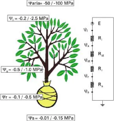
Similarly to an electric circuit, water flow in a plant can be described through a potential, resistance and capacitance network (Fig. 2.2).

Fig. 2.2. Scheme of potential, resistance and capacitance network for a plant water flow. Ψs is the soil water potential, Ψr the root water potential, Ψx the xylematic water potential,

Ψl the leaf water potential, Ψaria the atmosphere water potential, Rs the soil resistance, Rr

the root resistance, Rst the trunk resistance, Rl the leaf resistance, E the outside

environment (Mugnai, 2004).

The potential gradient in the soil-plant-atmosphere continuum (SPAC) is the force leading water transport through the plant: water flow will move from a high (less negative) water potential point to a lower (more negative) water potential point. So, water flow will normally follow the direction from the soil (_S 0.010.15MPa) towards the atmosphere (_atm50  100MPa) going through the plant (Mugnai, 2004).

Although not exactly analogous, comparisons between the soil–plant– atmosphere continuum and the flow of electricity through a resistance network has enhanced our understanding of the system (Coelho et al., 2003). Therefore, water movement through the SPAC is treated as a continuous process analogous to the flow of electricity in a conducting system and it is described by an analog of Ohm's Law, where Flow = Difference in water potential/Resistance. This is a logical extension of the cohesion theory of the ascent of sap (Kramer, 1974).

Soil water flow to plant roots has been studied by a great number of researchers. The microscopic approach considered the radial flow of water to a single root, and the macroscopic or whole root system approach assumed the soil-root system to be a continuum in which water flow is essentially one-dimensional flow. One of the greatest difficulties is to estimate the resistances along the pathway. In general, the resistance to water flow in the rhizosphere and within the roots is calculated using empirical equations (Coelho et al., 2003).

The SPAC approach provides a useful, unifying theory in which water movement through soil, roots, stems and leaves, and its evaporation into the air can be treated in terms of the driving forces and resistances operating at each stage. It also provides a model useful to investigators in analyzing the importance of various factors affecting water movement. Actually it is an oversimplification, because it assumes steady state conditions which seldom exist, and constant resistances, whereas root resistance appears to vary with rate of water flow. Furthermore, complications occur because movement in the liquid phase is proportional to difference in water potential (ΔΨ) and movement in the vapour phase is

concentration. However, these are minor problems compared to the over-all usefulness of the concept (Kramer, 1974).

3 Micrometeorological approaches for actual evapotranspiration measurement and estimation

From an energetic point of view, evapotranspiration can be considered as equivalent to the energy employed for transporting water from the inner cells of leaves and plant organs and from the soil to the atmosphere. In this case, it is called latent heat (λE, with λ latent heat of vaporization equal to 2.45x106 J kg-1 at 20 °C) and is expressed as energy flux density (W m-2). Under this form, evapotranspiration (ET) can be measured with the so called micrometeorological methods. These techniques are physically-based and depend on the laws of thermodynamics and of the transport of scalars into the atmosphere above the canopy. For applying the micrometeorological methods, it is usually necessary to accurately measure meteorological variables on a short temporal scale with sensors and suitable equipment placed above the canopy (Katerji and Rana, 2008).

There are a great variety of methods for measuring ET; some methods are more suitable than others because of their accuracy or cost or because they are particularly suitable for given space and time scales (Katerji and Rana, 2008).

Due to the conservative hypothesis of all the flux densities above the crop, the micrometeorological methods can be applied only on large flat surfaces with uniform vegetation. As a consequence, three conditions should be accurately analysed before using these techniques in the Mediterranean semi-arid region: i) advection, i.e. the contribution of supplementary energy (under the form of heat) from the dryer surrounding surfaces to the cropped surface by means of horizontal fluxes. This

the energy fluxes must be conservative, they can only be measured up to the height of the so-called internal boundary layer, i.e. the layer of air downwind of the leading edge affected by canopy. It interferes in particular through two parameters: the height of the canopy and its roughness length; iii) the position of the sensors above the canopy. They should be placed close enough to the canopy so to be inside the internal boundary layer, and far enough from the canopy allowing to appreciate larger gradients (Katerji and Rana, 2008).

Micrometeorological methods for measuring or estimating actual crop evapotranspiration are generally referred to a plot scale.

3.1 Eddy Covariance method

The transport of scalar (vapour, heat, CO2) and vectorial quantities (momentum) is mostly governed by air turbulence in the low atmosphere in contact with the canopies (Katerji and Rana, 2008). The Eddy Covariance (EC) method is a direct measure of a turbulent flux density of a scalar across horizontal wind streamlines (Paw U et al., 2000). It is very accurate with a large time resolution. However, it needs also the most comprehensive knowledge and great experimental effort (Foken, 2008a); some disadvantages include sensitivity to fetch and high cost and maintenance requirements (Brotzge and Crawford, 2003).

The calculation of turbulent fluxes is based on the Navier-Stokes equation and similar equations for temperature or gases by the use of the Reynolds' postulates. The equations for determination of surface fluxes are obtained by further simplifications. These are:

 stationarity of the measuring process, i.e. δX / δt = 0 (X represents the horizontal wind velocity u, the vertical wind velocity w, the temperature T and so on; t is the time);

 horizontal homogeneity of the measuring field, i.e. δX / δx = 0 and

δX / δy = 0 (x is the component into the direction of the mean wind, and y

is the component perpendicular to x);

 validity of the mass conservation equation, i.e. δw / δz = 0 and 0



w (z the height);

 negligible density flux, i.e. ρ' / ρ << 1 (with ρ the air density);  statistical assumptions, for example statistical independence and the definition of the averaging procedure;

 the Reynolds' postulates a' 0, ab' 0, abab and the postulate which is used for the calculation of the eddy covariance method

' 'b a b a ab   should be valid;

 the momentum flux in the surface layer as well as the temperature flux (analogue equations for water vapour and gaseous fluxes) doesn't change with the height within about 10% to 20% of the flux (Foken and Wichura, 1996).

The vertical component of the fluctuating wind is responsible for the flux across a plane above a horizontal surface. Since there is a net transport of energy across the plane, there will be a correlation between the vertical wind component and temperature or water vapour. For example, if water vapour is released into the atmosphere from the surface, updrafts will contain more vapour than downdrafts, and vertical velocity (positive upwards) will be positively correlated with vapour content (Drexler et al.,

The EC method is based on direct measurements of the product of vertical velocity fluctuations (w’) and scalar concentration fluctuations (c’) yielding a direct estimate of H and λE assuming that the mean vertical velocity is negligible. It provides estimates of H and λE separately, so that, when combined with measurements of RN and G, all the major components

of the energy balance are independently measured (Twine et al., 2000). So, a direct method for measuring the latent heat flux above a vegetative surface over a homogeneous canopy is to measure simultaneously vertical turbulent velocity and specific humidity fluctuations and to determine their covariance over a suitable sampling time. With these measurements, theory predicts that fluxes from the surface can be measured by correlating the vertical wind fluctuations from the mean (w’ in m s-1) with the fluctuations from the mean in concentration of the transported water vapour (q’ in kg m-3). So that, for latent heat we can write the following covariance of vertical wind speed and vapour density: ' 'q w E    (3.1)

If we take measurements of the instantaneous fluctuations of vertical wind speed w’ and humidity q’ at a frequency sufficient for obtaining the contribution from all the significant sizes of eddy, by summing their product over a hourly time scale, the above equation calculates the actual crop evapotranspiration. A representative fetch (distance from the canopy edge) is required; fetch to height ratios of 100 are usually considered adequate, but longer fetches are desirable. To measure ET with this method, vertical wind fluctuations must be measured and acquired at the same time as the vapour density. The first one can be measured by a sonic

anemometer; the second one by a fast response hygrometer (Katerji and Rana, 2008).

The sensible heat, H, using the EC technique by analogy with the expression above (Eq. 3.1), can be written as

' 'T

w c

H  _p (3.2)

with the air density and cp the specific heat of air at a constant pressure.

The wind speed and temperature fluctuations are measured by means of sonic anemometer and fast response thermometer, respectively (Katerji and Rana, 2008), so that the EC method requires sensitive, expensive instruments to measure high-frequency wind speeds and scalar quantities (Foken, 2008a).

Sensor must measure vertical velocity, temperature and humidity with sufficient frequency response to record the most rapid fluctuations important to the diffusion process. Typically, a frequency of the order of 5-10 Hz is used, but the response-time requirement depends on wind speed, atmospheric stability and the height of the instrumentation above the surface. Outputs are sampled at a sufficient rate to obtain a statistically stable value for the covariance (Drexler et al., 2004). If a 30-minute sampling time is used over the whole day, then remarkable errors will be reduced (Foken, 2008a).

Wind speed and humidity sensors should be installed close to each other but sufficiently separated to avoid interference. When the separation is too large, underestimation of the flux may result. High-frequency wind vector data are usually obtained with a triaxial sonic anemometer. The triaxial instruments provide the velocity vector in all three directions and, therefore, corrections can be applied for any tilt in the sensor and mean

systems including thermocouple psychrometers, Lyman-alpha and krypton hygrometers, laser-based systems and other infrared gas analysers (Drexler

et al., 2004). Since the size of the turbulence eddies increases with distance

above the ground surface, both the measuring path length and the separation between a sonic anemometer and an additional device (e.g. hygrometer) depend on the height of measurement. These additional instruments should be mounted downwind of the sonic anemometers, 5-10 cm below the measuring path. Therefore, to reduce the corrections of the whole system the measurement height must be estimated on the basis of both the path length of the sonic anemometer and the separation of the measuring devices. Also, the measuring height should be twice the canopy height in order to exclude effects of the roughness sublayer (Foken, 2008a).

The Eddy Covariance technique is the most direct method for quantifying the turbulent exchange of energy and trace gases between the Earth’s surface and the atmosphere (Mauder et al., 2010). However, the derivation of the mathematical algorithm is based on a number of simplifications so that the method can be applied only if these assumptions are exactly fulfilled. The quality of the measurements depends more on the application conditions and the exact use of the corrections than on the available highly sophisticated measuring systems. Therefore, experimental experience and knowledge of the special atmospheric turbulence characteristics have a high relevance. The most limiting conditions are: horizontally homogeneous surfaces and steady-state conditions (Foken, 2008a). These requirements are often violated in complex terrain, and their non-fulfilment reduces the quality of the measurement results. Foken and Wichura (1996) address this problem by assigning quality flags to the

fluxes in accordance with the deviations found between parameterisations under ideal conditions and those actually measured. Secondly, in a heterogeneous environment the land use types contributing to the measurements change with the source area of the fluxes. This source area, which can be calculated by footprint models, defines the region upwind of the measurement point which influences the sensor’s measurements and is dependent on measurement height, terrain roughness, and boundary layer characteristics, such as the atmospheric stability. As most sites in monitoring networks are set up to measure fluxes over a specific type of vegetation, the changing contribution of this type of land use, under different meteorological conditions, has to be considered in order to assess how representative the measurements are (Göckede et al., 2004).

The latter can lead to a bias of the flux estimate that becomes apparent in a lack of energy balance closure, usually ranging between 10 and 30% of the available energy at the surface. Several large-eddy simulations (LESs) support the thesis that single-tower eddy-covariance measurements, using temporal averaging, cannot completely represent the actual surface flux. According to these studies, the resulting flux bias depends on several factors, such as wind speed, measurement height, averaging time, degree of horizontal heterogeneity and atmospheric stability. Large-eddy simulation results show that the entire flux can be captured if spatial instead of, or in addition to, temporal averaging is applied when calculating the covariance (Mauder et al., 2010).

It is possible to minimize the deviation between actual and measured EC fluxes through an optimal equipment configuration and through application of adequate correction methods. The typical steps are: tilt

correction (also WPL correction, see Webb et al. 1980) and damping (attenuation) correction (Spank and Bernhofer, 2008).

The application of correction methods is closely connected with the data control; it starts with the exclusion of missing values and outliers. A basic condition for applying the EC method is the assumption of a negligible mean vertical wind component; otherwise advective fluxes must be corrected. This correction is called tilt correction and includes the rotation of a horizontal axis into the mean wind direction. The first correction is the rotation of the coordinate system around the z-axis into the mean wind. The second rotation is around the new y-axis until the mean vertical wind disappears. With these rotations, the coordinate system of the sonic anemometer is moved into the streamlines (Foken, 2008a).

The most commonly applied technique for determining the angles necessary to place the sonic anemometer into a streamwise coordinate system involves a series of two rotations, applied at the end of each turbulent averaging period. The first rotation sets v0 by swinging the x and y-axes about the z-axis so that the new velocities are given by

  sin cos 1 um vm u   (3.3)   cos sin 1 um vm v   (3.4) m w w ₁ (3.5) where         m m u v 1 tan  (3.6)

and where subscript m is for ‘measured’ and subscript 1 denotes the velocities after the first rotation. The second rotation sets w0 by

swinging the new x and z-axes about y so that the x-axis points in the mean streamline direction. The final velocities are then given by

  sin cos ₁ 1 2 u w u   (3.7) 1 2 v v  (3.8)   cos sin ₁ 1 2 u w w   (3.9) where         1 1 1 tan u w  (3.10)

The above double rotation aligns the x-axis with the mean wind vector, but allows the y and z-axes to freely rotate about x. That is, there are an infinite number of anemometer rotations that simultaneously satisfy

0   w

v . The anemometer’s final orientation in the y-z plane after the double rotation depends on its initial orientation (Wilczak et al., 2001).

This very commonly used method, involving a double rotation of the anemometers’ axes, is shown to result in significant run-to-run stress errors due to the sampling uncertainty of the mean vertical velocity (Wilczak et

al., 2001).

The previous analysis shows that if the error in the y-z plane is only 1 degree then the error in vw can be of the same order as the true stress.

Over land, a third sonic rotation can be applied to remove this ambiguity by requiring that vw0. In this step the new y and z-axes are rotated around x until the cross-stream stress becomes zero, and the third set of rotation equations then become

2 3 u u  (3.11)   sin cos w v v   (3.12)

where





This alternative method, requiring a triple rotation of the anemometer axes, is shown to result in even greater run-to-run stress errors due to the combined sampling errors of the mean vertical velocity and the cross-wind stress (Wilczak et al., 2001).

Another kind of rotation is the so called planar-fit method, that is a rotation into the mean stream lines. With this method, the differences between the measuring device and the mean stream field for an unchanged mounting of the anemometer is estimated over a long time period (days to weeks) for a given measuring place; this means that the measuring device must be orientated over this period without any changes. The planar-fit coordinate system fitted to the mean-flow streamlines is characterized by

0  p

w . After the rotation into the mean streamline level, each single measurement must be rotated into the mean wind direction (Foken, 2008a). It is shown to reduce the run-to-run stress errors due to sampling effects, and provides an unbiased estimate of the lateral stress (Wilczak et al., 2001).

An important correction to the actual available turbulence spectra is the adjustment of the spectral resolution of the measuring system. Hence, the resolution in time (time constant), the measuring path length, and the separation between different measuring paths must be corrected. The spectral correction is made using transfer functions (Foken, 2008a).

The so called WPL-correction is a density correction, caused by ignoring density fluctuations, a finite humidity flux at the surface, and the

unit. The WPL-correction is large if the turbulent fluctuations are small relative to the mean concentration. The conversion from volume into mass-related values using the WPL-correction is not applicable if the water vapour concentrations or the concentrations of other gases are transferred into mol per mol dry air before the calculation of the eddy-covariance. However, the calculation is possible depending on the sensor type and if it is offered by the manufacturers (Foken, 2008a).

Hence, the quality assurance of turbulence measurements with the EC method is a combination of the complete application of all corrections and the exclusion of meteorological influences such as internal boundary layers, gravity waves, and intermitted turbulence. Quality tests are used to validate the theoretical assumptions of the method such as steady-state conditions, homogeneous surfaces, and developed turbulence (Foken, 2008a).

3.2 Surface Renewal technique

It is difficult to achieve a good closure of the surface energy balance equation when all the energy fluxes are independently measured. This problem involves different shortcomings which are a matter of research. The footprint effect, which is the lack of coincidence of the source area among the terms of the surface energy balance measured using different instruments and techniques, is recognized as one of the problems in achieving a good closure. For determining the flux of a scalar, fetch requirements may depend on the method applied and while Eulerian analytical models and Lagrangian stochastic dispersion models are available, the well known rule of thumb 100:1 (fetch to height) is often

estimate scalar surface fluxes is based on the scalar conservation equation and requires the measurement of the scalar (at high frequency) taken at one height as input. The distance downwind from the leading edge needed to deploy instrumentation depends on the measurements required as input in the method used for scalar flux estimation (Castellví, 2012).

Traces of high-frequency temperature data show ramp-like structures resulting from turbulent coherent structures. The coherent structure theory assumes that an air parcel sweeps from above to the surface. The transfer between the air and the canopy elements lead to heating or cooling of the air while is at the surface. Because these fluctuations are coherent, ramps are observed when high-frequency temperature measurements are taken at a point at or above the canopy top. Two parameters characterize these mean temperature ramps for stable and unstable atmospheric conditions: the amplitude (a) and the inverse ramp frequency (l+s, with l the period with gradually increasing or decreasing temperature and s the quiescent period). The mean values of these two parameters during a time interval can be used to estimate H over several crop canopies using SR analysis (Snyder et al., 1996; Zapata and Martínez-Cob, 2001, 2002).

In SR analysis, a parcel of air is assumed to originate above the canopy with a characteristic scalar value (Chen et al., 1997b).

Consider an air parcel, with some scalar concentration, travelling at a given height above the surface. SR analysis assumes that at some instant the parcel suddenly moves down to the surface and remains connected with the sources (sinks) for a period of time during which it is horizontally travelling along the sources. By continuity, the parcel ejects upwards and is replaced by another parcel sweeping in from aloft. During the connect time with the surface, scalar transfers to or from the sources to the air parcel.