Delayed Theory Combination vs. Nelson-Oppen for Satisfiability Modulo Theories: a Comparative Analysis

UNIVERSITY

OF TRENTO

DEPARTMENT OF INFORMATION AND COMMUNICATION TECHNOLOGY

38050 Povo – Trento (Italy), Via Sommarive 14

http://www.dit.unitn.it

DELAYED THEORY COMBINATION VS. NELSON-OPPEN FOR

SATISFIABILITY MODULO THEORIES: A COMPARATIVE

ANALYSIS

Roberto Bruttomesso, Alessandro Cimatti, Anders Franzén

Alberto Griggio and Roberto Sebastiani

May 2006

Delayed Theory Combination vs. Nelson-Oppen for

Satisfiability Modulo Theories: a Comparative Analysis

?

Roberto Bruttomesso1_{, Alessandro Cimatti}1_{, Anders Franzen}1,2_,

Alberto Griggio2, and Roberto Sebastiani2

1_{ITC-IRST, Povo, Trento, Italy.{bruttomesso,cimatti,franzen}@itc.it} 2_{DIT, Universit`a di Trento, Italy.{griggio,rseba}@dit.unitn.it}

Abstract. Many approaches for Satisfiability Modulo Theory (SMT(T)) rely on the integration between a SAT solver and a decision procedure for sets of liter-als in the background theoryT (T-solver). WhenT is the combinationT1∪T2

of two simpler theories, the approach is typically handled by means of Nelson-Oppen’s (NO) theory combination schema in which two specificT-solvers de-duce and exchange (disjunctions of) interface equalities.

In recent papers we have proposed a new approach to SMT(T1∪T2), called

De-layed Theory Combination (DTC). Here part or all the (possibly very expensive) task of deducing interface equalities is played by the SAT solver itself, at the potential cost of an enlargement of the boolean search space. In principle this enlargement could be up to exponential in the number of interface equalities gen-erated.

In this paper we show that this estimate was too pessimistic. We present a com-parative analysis of DTCvs. NO for SMT(T1∪T2), which shows that, using

state-of-the-art SAT-solving techniques, the amount of boolean branches performed by DTCcan be upper bounded by the number of deductions and boolean branches performed by NO on the same problem. We prove the result for different deduc-tion capabilities of theT-solvers and for both convex and non-convex theories.

1 Introduction

Satisfiability Modulo a Theory

T

(SMT(

T

)) is the problem of checking the satisfiability of a quantifier-free (or ground) first-order formula with respect to a given first-order theory

T

. Theories of interest for many applications are, e.g., the theory of difference logic

DL

, the theory

EUF

of equality and uninterpreted functions, the quantifier-free fragment of Linear Arithmetic over the rationals

LA

(Q) and that over the integers

LA

(Z). Particularly relevant is the case of SMT(

T

1∪

T

2), where the background theory

T

is the combination of two (or more) simpler theories

T

1and

T

2.1

?_{This work has been partly supported by ISAAC, an European sponsored project, contract no.} AST3-CT-2003-501848, by ORCHID, a project sponsored by Provincia Autonoma di Trento, and by a grant from Intel Corporation.

1_{For better readability, and as it is common practice in papers dealing with combination of} the-ories, in this paper we always deal with only two theoriesT1andT2. The discourse generalizes to more than two theories.

A prominent approach to SMT(

T

) which underlies several systems (e.g., CVCLITE

[2], DLSAT [8], DPLL(T)/BarceLogic [10], MATHSAT [4], TSAT++ [1], ICS/YICES

[9]), is based on extensions of propositional SAT technology: a SAT engine is modified to enumerate boolean assignments, and integrated with a decision procedure for sets of literals in the theory

T

(

T

-solver). The above schema is also followed to tackle the SMT(

T

1∪

T

2) problem. The approach relies on a decision procedure able to decide

the satisfiability of sets of literals in

T

1∪

T

2, that is typically based on an integration

schema like Nelson-Oppen (NO) [11] (or its variant due to Shostak [13]): the

T

i-solvers

are combined by means of a structured exchange of (disjunctions of) interface equalities (ei j’s).

Unfortunately from a practical point of view this schema poses some challenges. First, the integration between the two

T

i-solvers is not trivial to implement. Second,

the ability of

T

i-solvers of inferring (disjunctions of) interface equalities (hereafter ei j -deduction completeness) required by NO is neither always easy to achieve nor always cheap to perform. (E.g., ei j-deduction is cheap for

EUF

but can be very expensive for

LA

(Z).) Third, in case of non-convex theories (e.g.,

LA

(Z)), a backtrack search must be used to take care of the disjunctions that need to be managed.

In recent papers [3, 6] we have proposed a novel approach to SMT(

T

1∪

T

2), called

Delayed Theory Combination (DTC). The main idea is to avoid the integration schema between

T

1and

T

2, and tighten the connection between each

T

iand the SAT engine.

While the truth assignment is being constructed, it is checked for consistency with re-spect to each theory in isolation. This can be seen as constructing two (possibly incon-sistent) partial models for the original formula; the “merging” of the two partial models is enforced, on demand, since the solver is requested to find a complete assignment to the ei j’s.

Compared to the NO schema, this approach has several advantages [3, 6]. First, it is easier to implement and analyze. Second, the approach does not rely on the

T

i-solvers

being ei j-deduction complete, although it can fully benefit from this property. Third, the

DTCnicely encompasses the case of non-convex theories. On the negative side, in [3,

6] we noticed that these benefits are traded with a potential enlargement of the boolean search space which, in principle, could be up to exponential in the number of interface equalities generated. Thus, despite the positive empirical results presented in [3, 6], the latter fact represented, at least in theory, one possible drawback of DTC.

In this paper we show that this latter point was way too pessimistic. We present a comparative analysis of DTCvs. NO for SMT(

T

1∪

T

2), and we introduce some novel

theoretical results, for both convex and non-convex theories and for different deduction capabilities of the

T

-solvers. These results show that, by exploiting the full power of advanced SAT techniques like backjumping and learning, DTCcan be implemented in

such a way as to mimic the behavior of NO, so that the amount of boolean branches required by DTC can be upper-bounded by the sum of the number of deductions and

branches required by NO in order to perform the same tasks.

From these results we have that DTCgeneralizes NO, in the sense that:

– under the same hypotheses of ei j-deduction-completeness of the

T

i-solvers required

– in the more general case (

T

i-solvers with partial or no ei j-deduction capabilities)

DTC can mimic the behavior of NO, in such a way that all or part of the

(pos-sibly very expensive) ei j-deductions are substituted with only few extra boolean

branches.

We also notice that the capability of learning conflict clauses containing interface equal-ities, which is typical of DTC, allows for cutting branches corresponding to repeated deductions in an equivalent NO schema.

The paper is structured as follows. In Section 2 we present some background and introduce the Nelson-Oppen combination schema for SMT(

T

1∪

T

2). DTCis then

dis-cussed in Section 3. We present our analysis in Sections 5 (where the case of ei j

-deduction completeness in the

T

i-solvers of DTC is examined) and 4 (where the

T

i

-solvers employed by DTCare assumed to have limited or no deduction capabilities).

Finally, in Section 6 we draw some conclusions. The proofs of the theorems are reported in appendix.

2 SMT for combined theories via Nelson-Oppen’s integration

2.1 Basic definitions and properties

Consider a theory

T

with equality.

T

is stably-infinite iff every quantifier-free

T

-satisfiable formula is -satisfiable in an infinite model of

T

. Notice that

EUF

,

DL

(Q),

DL

(Z),

LA

(Q),

LA

(Z) are stably-infinite, whereas e.g. theories of bit-vectors

BV

are typically not. In what follows, we shall assume to deal only with stably-infinite theories with equality and with disjoint signatures.

T

is convex iff, for every collection l1, ..., lk, e, e0of literals in

T

s.t. e, e0are in the

form (x = y), x, y being variables, we have that

{l1, ..., lk} |=T (e ∨ e0) ⇐⇒ {l1, ..., lk} |=T e or {l1, ..., lk} |=T e0.

Notice that

EUF

,

DL

(Q),

LA

(Q) are convex, whereas

DL

(Z) and

LA

(Z) are not. Consider two theories

T

1,

T

2with equality and disjoint signatures Σ1, Σ2. An atom

ψ is i-pure if only =, variables and symbols from Σioccur in ψ. A formula ϕ is pure iff

every atom in ϕ is i-pure for some i ∈ {1, 2}. Every non-pure

T

1∪

T

2formula ϕ can be

converted into an equivalently satisfiable pure formula ϕ0_{by recursively labeling terms} t with fresh variables vt, and by adding the atom (vt= t). E.g.:

( f (x+3y) = g(2x−y)) ⇒ ( f (vx+3y) = g(v2x−y))∧(vx+3y= x+3y)∧(v2x−y= 2x−y).

This process is called purification, and is linear in the size of the input formula. Thus, henceforth we assume w.l.o.g. that all input formulas ϕ ∈

T

1∪

T

2are pure.

If ϕ is a pure

T

1∪

T

2formula, then v is an interface variable for ϕ iff it occurs in

both 1-pure and 2-pure atoms of ϕ. An equality (vi= vj) is an interface equality for ϕ

iff vi, vjare interface variables for ϕ. We assume an unique representation for (vi= vj)

and (vj= vi). Henceforth we denote the interface equality (vi= vj) by “ei j”.

Given a

T

-inconsistent set of literals L = {l1, . . . , ln} in a theory

T

, a conflict set

η is an (

T

-)inconsistent subset of L. η is minimal if none of its strict subsets is

T

-inconsistent. We say that η is ¬ei j-minimal iff η \ {¬ei j} is no more

T

-inconsistent, for

function Bool+T (ϕ: quantifier-free formula) 1 Ap_{←−T2B(Atoms(ϕ))}

2 ϕp_{←−T2B(ϕ)}

3 while Bool-satisfiable(ϕp_{) do} 4 µp_{←− pick total assign(A}p_{, ϕ}p₎ 5 (ρ, π)←−T− satis f iable(B2T(µp₎₎ 6 if ρ = sat then return sat

7 ϕp_{←− ϕ}p_∧T2B(¬π) 8 end while

9 return unsat end function

Fig. 1. A simplified view of enumeration-based T-satisfiability procedure: Bool+T

A

T

-solver is a procedure that decides the consistency of an assignment µ in

T

. An (propositional) assignment µ for a formula ϕ is a function µ : Atoms(ϕ) 7→ {true, f alse}. µ can be equivalently represented as a set of literals µS, where ¬A ∈ µSif µ(A) = f alse,

and A ∈ µS otherwise. µ can also equivalently be seen as a formula µϕ, built as the

conjunction of the literals in the set µS. (In the following, we will denote all such

equiv-alent representations with µ. Moreover, we will denote with µTithe subassignment of µ

containing only i-pure literals.) When a

T

-solver detects the inconsistency of µ, it also returns a conflict set η of µ. Finally, we also require every

T

-solver involved in either the NO schema or DTCto be incremental (it does not need to restart the computation

from scratch to decide the satisfiability of µ0_{if it had already proved that of µ ⊂ µ}0_{) and} backtrackable (it can return to a previous state in an efficient manner) [11].

We say that a

T

-solver is ¬ei j-minimal (resp. minimal) if the conflict sets it returns

are always ¬ei j-minimal (resp. minimal). Notice that ¬ei j-minimality is a much weaker

requirement than minimality.

2.2 Satisfiability Modulo Theory

Fig. 1 presents Bool+

T

, a (much simplified) decision procedure for SMT(

T

). The function Atoms(ϕ) takes a ground formula ϕ and returns the set of atoms which occur in ϕ. We use the notation ϕp to denote the propositional abstraction of ϕ, which is formed by the function

T

2

B

that maps propositional variables to themselves, ground atoms into fresh propositional variables, and is homomorphic w.r.t. boolean operators and set inclusion. The function

B

2

T

is the inverse of

T

2

B

. We use µp _{to denote a}

propositional assignment. (If

T

2

B

(µ) |=

T

2

B

(ϕ), then we say that µ propositionally satisfies ϕ.) The idea underlying the algorithm is that the truth assignments for the propositional abstraction of ϕ are enumerated and checked for satisfiability in

T

. The procedure either returns sat if one such model is found, or returns unsat otherwise. The function pick total assign returns a total assignment to the propositional variables in ϕp_{, that is, it assigns a truth value to all variables in}

_A

p_{. The function}

_T

_{-satisfiable(µ)}

returns (unsat, π), where π ⊆ µ is a

T

-unsatisfiable set, called a theory conflict set. We call the negation of a conflict set, a conflict clause.

The algorithm is a coarse abstraction of the ones underlying TSAT++, MATHSAT,

DLSAT, DPLL(T)/BarceLogic, CVCLITE, and ICS/YICES. The test for

satisfiabil-ity and the extraction of the corresponding truth assignment are kept separate in this description only for the sake of simplicity.

In practice, the enumeration of truth assignments is carried out by means of effi-cient implementations of the DPLL algorithm [15], where a partial assignment µp_is

built incrementally, each time selecting an unassigned literal l (literal selection), called decision literal, according to some heuristic criterion, adding it to µp_{and performing}

all the other assignments which derive deterministically from this choice (unit propaga-tion). When some assignment µp_{falsifies the formula returning a (boolean) conflict set}

πp_{, or when}

_T

_{-satisfiable(}

_B

₂

_T

_(µp_{)) fails returning a theory conflict set π, the negation} ¬πp_{of (the boolean abstraction of) the conflict set is passed as a conflict clause to the}

boolean solver. Then ¬πp_{is added in conjunction to ϕ}p_{either temporarily or}

perma-nently (learning), and the algorithm backtracks up to the highest point in the search where a literal can be unit-propagated on ¬πp _{(backjumping). Learning also avoids}

generating the same conflicts in future branches.

An important variant [10] is that of building from ¬πp_{a “mixed boolean+theory}

conflict clause”, by recursively removing non-decision literals l from the conflict clause by resolving the latter with the clause Cl which caused the unit-propagation of l; this

is done until the conflict clause contains only decision literals (last-UIP strategy) or at most one non-decision literal assigned after the last decision (first-UIP strategy).2

Another important improvement is early pruning (EP): before every literal selec-tion, intermediate assignments are checked for

T

-satisfiability and, if not

T

-satisfiable, they are pruned (since no refinement can be

T

-satisfiable). Finally, theory deduction can be used to reduce the search space by allowing the

T

-solvers to explicitly return truth values for unassigned literals, which can be unit-propagated by the SAT solver. The interested reader is pointed to, e.g., [1, 4, 10, 5] for details and further references.

2.3 Nelson-Oppen’s schema

Given two signature-disjoint stably infinite theories

T

1and

T

2, the Nelson-Oppen

com-bination schema [11], in the following referred to as NO, allows for solving the satisfia-bility problem for

T

1∪

T

2(i.e. the problem of checking the

T

1∪

T

2-satisfiability of sets

of Σ1∪ Σ2-literals) by using the satisfiability procedures for

T

1and

T

2. The procedure is

basically a structured interchange of information inferred from either theory and prop-agated to the other, until convergence is reached. The schema requires the exchange of information, the kind of which depends on the convexity of the involved theories. In the case of convex theories, the two solvers communicate to each other single interface equalities. In the case of non-convex theories, the NO schema becomes more com-plicated, because the two solvers need to exchange arbitrary disjunctions of interface equalities, which have to be managed within the decision procedure by means of case

2_{These are standard techniques implemented in most SAT solvers in order to build the boolean} conflict clauses [14].

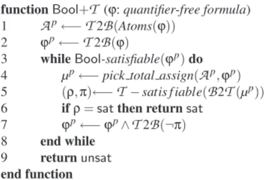
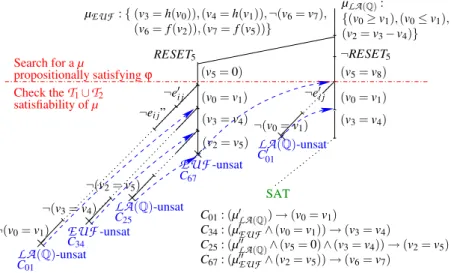
Branch 1 Branch 2 ¬RESET5 v0= v1 v2= v5 v3= h(v0) v4= h(v1) v6= f (v2) v7= f (v5) v3= v4 ¬(v6= v7) v0≥ v1 v5= 0 v0= v1 v2= v5 v3= v4 v2= v3− v4 v0≥ v1 v5= v8 v0≤ v1 v0= v1 v3= v4 v2= v3− v4 v3= h(v0) v4= h(v1) v6= f (v2) v7= f (v5) v0= v1 v3= v4 ¬(v6= v7) v0≤ v1 LA(Q) EUF∪LA(Q)-Satisfiable! EUF EUF LA(Q) hei j-deductioni hei j-deductioni hei j-deductioni hei j-deductioni hei j-deductioni RESET5

Fig. 2. Representation of the search tree for the formula of Example 1

splitting and of backtrack search. In the latter case, the NO schema performs a number of branches to check the consistency of a set of literals which depends on how many disjunctions of equalities are exchanged at each step: if the current set of literals is µ, and one of the

T

i-solver sends the disjunction Wnk=1(ei j)k to the other, the latter must

further investigate up to n branches to check the consistency of each of the µ ∪ {(ei j)k}

sets separately.

We notice that the ability to carry out deductions of (disjunctions of) ei j’s is crucial

for NO: if the current set of literals µTi in input to each

T

i-solver is

T

i-consistent, then

T

i-solver must be able to derive the (disjunctions of) interface equalities ei jwhich are

entailed by µTi in

T

i(if any), or say that no (disjunction of) ei j’s is entailed if this is

the case. If the

T

i-solver is always capable of doing this, we say that it is ei j-deduction complete. In what follows we will assume that all the

T

i-solvers used in a NO schema

are ei j-deduction complete.

Example 1 (convex case). Consider the following

EUF

∪

LA

(Q) formula ϕ (see Fig. 2)

EUF

: (v3= h(v0)) ∧ (v4= h(v1)) ∧ (v6= f (v2)) ∧ (v7= f (v5))∧

LA

(Q) : (v0≥ v1) ∧ (v0≤ v1) ∧ (v2= v3− v4) ∧ (RESET5→ (v5= 0))∧

Both : (¬RESET5→ (v5= v8)) ∧ ¬(v6= v7).

(1)

v0, v1, v2, v3, v4, v5are interface variables, v6, v7, v8are not. (Thus, e.g., (v0= v1) is an

interface equality, whilst (v0= v6) is not.) RESET5is a boolean variable.

After the first run of unit propagations, assume DPLL selects the literal RESET5,

re-sulting in the assignment

µ = { (v3= h(v0)), (v4= h(v1)), (v6= f (v2)), (v7= f (v5)), (v0≥ v1),

(v0≤ v1), (v2= v3− v4), ¬(v6= v7), RESET5, (v5= 0)}, (2)

which propositionally satisfies ϕ. Now, the set of literals µEUF ⊂ µ is given to the

EUF

solver, which reports its consistency and deduces no new interface equality. Then the set µ_LA(Q)⊂ µ is given to the

LA

(Q) solver, which reports consistency and deduces the

interface equality (v0= v1), which is passed to the

EUF

solver. The new set µEUF∪ {(v0= v1)} is still

EUF

-consistent, but this time the

EUF

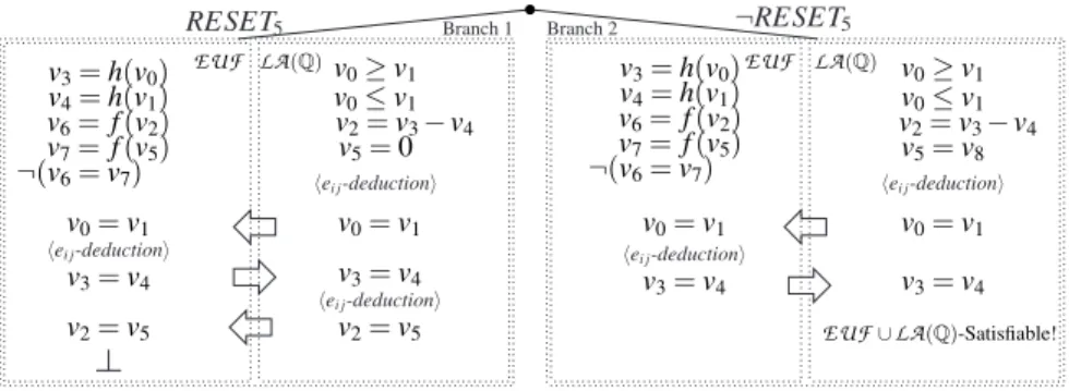
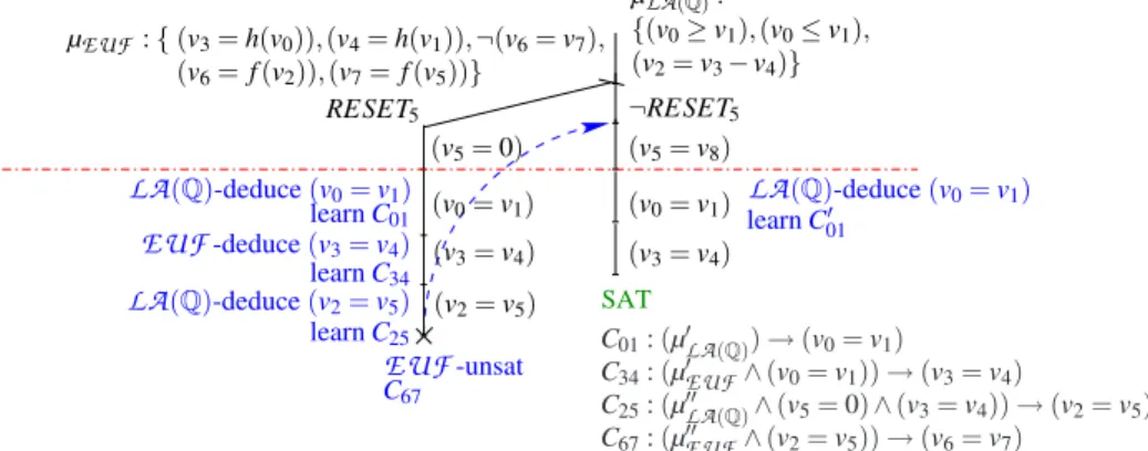
solver deduces the equality

v2= v3∨ v2= v4 v1= v3∨ v1= v4 v1≥ 0 v1≤ 1 v2≥ v6 v2≤ v6+ 1 v4= 1 v3= 0 v5= v4− 1 v5= v6 v2= v3 v1= v4 v1= v3 v5= v6 v2= v4 ¬( f (v2) = f (v4)) f (v3) = v5 f (v1) = v6 ¬( f (v1) = f (v2)) µLA(Z) EUF∪LA(Z)-Satisfiable! µEUF hei j-deductioni hei j-deductioni hei j-deductioni

Fig. 3. Representation of the search tree for the formula of Example 2

(v3= v4), which is in turn passed to the

LA

(Q) solver, that now as a consequence of this

and the assignment µ_LA(Q)deduces (v2= v5). The

EUF

solver is then invoked again

to check the

EUF

-consistency of the assignment µEUF∪ {(v0= v1), (v2= v5)}: since

this check fails, the Nelson-Oppen method reports the

EUF

∪

LA

(Q)-unsatisfiability of ϕ under the whole assignment µ. At this point, then, DPLL backtracks and tries assigning false to RESET5, resulting in the new assignment

µ = { (v3= h(v0)), (v4= h(v1)), (v6= f (v2)), (v7= f (v5)), (v0≥ v1), (v0≤ v1),

(v2= v3− v4), ¬(v6= v7), ¬RESET5, (v5= v8))},

which is found

EUF

∪

LA

(Q)-satisfiable (see Fig. 2). ¦

Example 2 (non-convex case). Consider the following

EUF

∪

LA

(Z) formula ϕ

EUF

: ¬( f (v1) = f (v2)) ∧ ¬( f (v2) = f (v4)) ∧ ( f (v3) = v5) ∧ ( f (v1) = v6)∧

LA

(Z) : (v1≥ 0) ∧ (v1≤ 1) ∧ (v5= v4− 1) ∧ (v3= 0) ∧ (v4= 1)∧

(v2≥ v6) ∧ (v2≤ v6+ 1).

(3)

Here (see Fig. 3) all the variables (v1, . . . , v6) are interface ones. ϕ contains only unit

clauses, so after the first run of unit propagations, DPLL generates the assignment µ which is simply the set of literals in ϕ. The Nelson-Oppen combination schema then runs as follows. First, the sub-assignment µEUF is given to the

EUF

solver, which reports its consistency and deduces no interface equality. Then, the sub-assignment µLA(Z) is given to the

LA

(Z) solver, which reports its consistency and deduces the

disjunction (v1= v3) ∨ (v1= v4). Next, there is a case-splitting and the two

equal-ities (v1= v3) and (v1= v4) are passed to the

EUF

solver. The first branch,

cor-responding to selecting (v1 = v3), is opened: then the set µEUF ∪ {(v1= v3)} is

EUF

-consistent, and the equality (v5= v6) is deduced. After that, the assignment

µLA(Z)∪ {(v5= v6)} is passed to the

LA

(Z) solver, that reports its consistency and

de-duces another disjunction, (v2= v3) ∨ (v2= v4). At this point, another case-splitting is

function Bool+T1+T2(ϕi: quantifier-free formula) 1 ϕ ←− purify(ϕi)

2 Ap_{←−T2B(Atoms(ϕ) ∪ interface equalities(ϕ))} 3 ϕp_{←−T2B(ϕ)}

4 while Bool-satisfiable (ϕp_{) do}

5 µp₁∧ µp₂∧ µep= µp←− pick total assign(Ap, ϕp) 6 (ρ1, π1)←−T1-satisfiable (B2T(µ1p∧ µ

p e)) 7 (ρ2, π2)←−T2-satisfiable (B2T(µ2p∧ µpe)) 8 if (ρ1= sat ∧ ρ2= sat) then return sat else 9 if ρ1= unsat then ϕp←− ϕp∧T2B(¬π1) 10 if ρ2= unsat then ϕp←− ϕp∧T2B(¬π2) 11 end while

12 return unsat end function

Fig. 4. A simplified view of the Delayed Theory Combination procedure for SMT(T1∪T2)

and µEUF ∪ {(v1= v3), (v2= v4)}. Both of them are found inconsistent, so the whole

branch previously opened by the selection of (v1= v3) is found inconsistent; at this

point, the other case of the branch (i.e. the equality (v1= v4)) is selected, and since

the assignment µEUF ∪ {(v1= v4)} is

EUF

-consistent and no new interface equality

is deduced, the Nelson-Oppen method reports the

EUF

∪

LA

(Z)-satisfiability of ϕ

under the whole assignment µ. ¦

3 SMT for combined theories via Delayed Theory Combination

In the Delayed Theory Combination (DTC) schema [3, 6], the SMT(

T

1∪

T

2) problem is

tackled in a different way: instead of using the Nelson-Oppen schema to combine two decision procedures for

T

1and

T

2by exchange of (disjunctions of) interface equalities,

each of the two

T

isolvers works in isolation, without direct exchange of information.

Their mutual consistency is ensured by augmenting the input problem with all interface equalities ei j, even if these do not occur in the original problem. The enumeration of

assignments includes not only the atoms in the formula, but also the interface equalities ei j. Both theory solvers receive, from the boolean level, the same truth assignment µefor ei j: under such conditions, the two “partial” models found by each decision procedure

can be merged into a model for the input formula.

A simplified view of the algorithm is presented in Fig. 4. Initially (lines 1–3), the formula is purified, the new ei j’s are created and added to the set of propositional

sym-bols

A

p_{, and the propositional abstraction ϕ}p_{of ϕ is created. Then, the main loop is}

entered (lines 4–11): while ϕp_{is propositionally satisfiable (line 4), a satisfying truth}

assignment µp_{is selected (line 5). It is important to stress that truth values are}

associ-ated not only to atoms in ϕ, but also to the ei jatoms, even though they do not occur in

ϕ. µp_{is then (implicitly) separated into µ}p

1∧ µpe∧ µ2p, where

B

2

T

(µip) is a set of i-pure

literals and

B

2

T

(µep) is a set of ei j-literals. The relevant parts of µpare checked for

ρiis unsat iff µ is unsatisfiable in

T

i, and sat otherwise. If both calls to

T

i-satisfiable

re-turn sat, then the formula is satisfiable. Otherwise, when ρiis unsat, then πiis a theory

conflict set, i.e. πi⊆ µ and πi is

T

i-unsatisfiable. Then, ϕpis strengthened to exclude

truth assignments which may fail in the same way (line 9–10), and the loop is resumed. Unsatisfiability is returned (line 12) when the loop is exited without having found a model.

In practical implementations of DTC, the search for a satisfactory assignment is

based on a modern DPLL engine, performing literal selection, unit-propagation, back-jumping and learning, early pruning, and theory deduction, as explained in §2.2. In particular, DTCcan be enhanced by ei j-deduction, in which ei j’s can by deduced by the

T

i-solvers and hence unit-propagated. (See Step 4. of Strategy1 below). We refer the

reader to [3, 6] for a more detailed discussion.

Notation-wise, we call “new” ei j’s all the interface equalities ei j’s which do not

occur in any clause of the input formula ϕ (including all the clauses learned). Moreover, we often write sets of literals {l1, ..., ln} as conjunctions l1∧ ... ∧ ln, and we often write

clauses (W_ili) ∨ (Wjlj) as implications: (Vi¬li) → (Wjlj) or (Vi¬li∧Vj¬lj) → ⊥.

Hereafter, for the sake of proving the theoretical results in §4 and §5, we assume that DTCimplements the following strategy.

Strategy 1 (NO emulation)

1. All the conflict clauses derived by theory conflicts are learned, either temporarily or permanently.3

2. Each conflict clause in 1. is a mixed boolean+theory conflict clause which is built from the theory conflict set by means of the last-UIP strategy described in §2.2.4

3. The literal selection heuristic and the

T

i-solvers calls are such that:

(i) new ei j’s are selected only after all the other literals have been assigned,

(ii) Early pruning (EP) is applied before every selection of a new ei j,5

(iii) the new ei j’s selected are always assigned false,

(iv) each

T

i-solver is invoked only if at least one literal (which has not been deduced singularly by

T

i-solver itself) has been added to its input since the last call.6

4. At every early-pruning call on a branch (namely µ) which is found both

T

1- and

T

2

-consistent, if one

T

i-solver performs the ei j-deduction µ∗|=Ti W_k

j=1ej, s.t. µ∗⊆ µTi,

each ejbeing an unassigned interface equality on variables in µ, then:

(i) the clause

T

2

B

(µ∗_→Wk

j=1ej) is learned immediately;

3_{That is, if oneT}

i-solver returns a conflict set π, then the conflict clausesT2B(¬π) is always added to ϕp_{, either temporarily or permanently.}

4_{That is, each conflict clause contains all and only (the negation of) the decision literals which} forced the unit-propagation or the ei j-deduction of those in the theory conflict.

5_{That is, before selecting and adding a new (negated) e}

i jto µ, theTi-satisfiability of µ is checked for bothTi’s by calling theTi-solver’s. If µ is foundTi-inconsistent for someTi, then the procedure backtracks.

6_{This avoids invoking aT}

i-solver twice in sequence on the same input. The restriction “which ... byTi-solver itself” means that, ifTi-solver (µ) returns “Sat” and deduces ei j, thenTi-solver is not invoked on µ ∪ {ei j}.

(ii) if k = 1, then ekis added to the current assignment and unit-propagated imme-diately;

(iii) if k > 1, then ¬e1, ..., ¬ekare put on the top of the literal selection list, so that to be the next ¬ei j’s selected by the literal selection heuristic.

5. [If and only if both

T

i-solvers are ei j-deduction complete]

If a total assignment µ which propositionally satisfies ϕ is found

T

i-satisfiable for both

T

i’s, and neither

T

i-solver performs any ei j-deduction from µ, then DTCstops returning “Sat”.7

4 DTC with non e

i j

-deduction-complete

T

i

-solvers vs. NO

In this section, we assume that both the

T

i-solvers employed by DTCare ¬ei j-minimal

and have limited or no ei j-deduction capabilities. Under these assumptions, we have the

following result.

Theorem 1. Let

T

1 and

T

2be two stably-infinite (possibly non-convex) theories. Let

both

T

i-solvers be ¬ei j-minimal, and possibly have some ei j-deduction capabilities; let

ϕ be a pure

T

1∪

T

2formula and let µ be a total assignment propositionally satisfying ϕ.

Let DTCwith Strategy 1 prove the

T

1∪

T

2-consistency (resp.

T

1∪

T

2-inconsistency) of

µ, returning a conflict set η in the case of inconsistency. Let dtc br and dtc ded be the number of boolean branches and of ei j-deductions performed in the DTCproof. Then we have:

dtc br + dtc ded ≤ no br + no ded, (4)

no ded and no br being respectively the number of deductions and of branches per-formed by a corresponding NO proof of the

T

1∪

T

2-consistency (resp.

T

1∪

T

2-inconsistency)

of µ.

Theorem 1 states that, if the

T

i-solvers are both ¬ei j-minimal, then there is a strategy

for DTCwhich emulates some NO proof (even though the

T

i-solvers have limited or no ei j-deduction capabilities!) at the cost of (at most) one extra boolean branch for every ei j-deduction performed by NO. Therefore the (possibly very expensive) ei j-deduction

steps of the NO schema can be avoided at the cost of one extra boolean branch each. More generally, we notice that one key idea in the proof of Theorem 1 is that, when the DPLL engine fails and generates a conflict set π, it backjumps up to the second-most-recently-assigned ¬ei j in π, if any [7]. (See, e.g., the case of C23 in Figure 6.)

Therefore, in a more general case than that of Theorem 1 (no ¬ei j-minimality), the more redundant ¬ei j’s the

T

i-solvers are able to remove from the conflict set returned, the more boolean branches are skipped by backjumping.

We consider some relevant subcases. Assume both

T

i-solvers have no deduction

capabilities. If so, dtc ded = 0. If

T

1,

T

2are both convex theories, then NO proves the

T

1∪

T

2-(un)satisfiability of µ by a chain of ei j-deductions in one branch (i.e., no br = 1).

From Theorem 1 we have dtc br ≤ no ded + 1.

7_{Step 5. is identical to theT}

SAT LA(Q)-unsat C01 C01: (µ0_LA(Q)) → (v0= v1) C34: (µ0EUF∧ (v0= v1)) → (v3= v4) C25: (µ00LA(Q)∧ (v5= 0) ∧ (v3= v4)) → (v2= v5) C67: (µ00EUF∧ (v2= v5)) → (v6= v7) LA(Q)-unsat C0 01 ¬(v3= v4) ¬(v2= v5) (v3= v4) (v2= v5) C67 C25 C34 ¬e0 i j RESET5 LA(Q)-unsat (v0= v1) (v5= 0) Check theT1∪T2 propositionally satisfying ϕ Search for a µ satisfiability of µ EUF-unsat ¬RESET5 (v0= v1) (v3= v4) (v5= v8) ¬(v0= v1) ¬ei j” ¬(v0= v1) EUF-unsat µ_LA(Q): {(v0≥ v1), (v0≤ v1), (v2= v3− v4)} µEUF : { (v3= h(v0)), (v4= h(v1)), ¬(v6= v7), (v6= f (v2)), (v7= f (v5))} ¬e0 i j

Fig. 5. DTC execution of Example 3 onLA(Q) ∪EUF, with no ei j-deduction. The clauses Ci j’s are the same as those of Fig. 7.

Example 3 (no ei j-deduction, convex case). Consider the

EUF

∪

LA

(Q) formula ϕ

(1) and the assignment µ (2) of Example 1. Look at Fig. 5. Both µLA(Q)and µEUF are

found consistent in the respective theories by the respective solvers.

Then DTCstarts selecting the new negated ei j’s, and proceeds without causing

con-flicts, until it selects ¬(v0= v1), which causes a

LA

(Q) conflict. As

LA

(Q) is

con-vex and

LA

(Q)-Solver is ¬ei j-minimal, it returns a conflict set in the form µ0_LA(Q)∪ {¬(v0= v1)} s.t. {(v0≥ v1), (v0≤ v1)} ⊆ µ0_LA(Q)⊆ µLA(Q). Thus DTClearns the

cor-responding clause C01and backjumps up to µ (or even higher), hence unit propagating

(v0= v1).

What happens next depends on whether the learned clause C01contains the

redun-dant

LA

(Q) atom (v5= 0) or not. Here (Fig. 5) we consider the “worst” case, that

is, when such atom is present in C01. This means that DTCbackjumps after the

unit-propagation of (v5= 0)8. Then (v0= v1) is unit-propagated and new unassigned ¬ei j’s

are selected again, until ¬(v3= v4) generates another conflict represented by clause

C34, which causes backjumping and unit-propagating (v3= v4). The same is repeated

for (v2= v5). Then µ ∪ {(v0= v1), (v3= v4), (v2= v5)} is found

EUF

-inconsistent

s.t. the conflict is represented by the clause C67, and the whole procedure backtracks,

causing the unit-propagation of ¬RESET5and (v5= v8)) as in Example 5.

We notice that, so far, the whole process mimics the NO deduction process of the first branch in Example 1 (see Fig. 2), requiring a number of extra boolean branches equal to the number of deductions performed by the corresponding NO process (dtc br = 4, dtc ded = 0, no br = 1 and no ded = 3.)

8_{More precisely, by Step 2. of Strategy 1, DTCeliminates (v}

5= 0) from the conflict clause

C01by resolving the latter with the clause RESET5→ (v5= 0) in ϕ, and thus by introducing

f (v1) = v6 ¬( f (v1) = f (v2)) ¬( f (v2) = f (v4)) f (v3) = v5 ¬(v1= v4) ¬(v1= v3) v2= v3 ¬(v2= v3) ¬(v2= v4) v1= v3 v5= v6 v2= v4 v1= v4 ¬(v5= v6) v1≥ 0 v1≤ 1 v2≥ v6 v2≤ v6+ 1 v5= v4− 1 v3= 0 v4= 1 µEUF: µLA(Z): LA(Z)-unsat, C13 EUF-unsat, C56 LA(Z)-unsat, C23 EUF-unsat, C14 EUF-unsat, C24 C13: (µ0_LA(Z)) → ((v1= v3) ∨ (v1= v4)) C56: (µ0EUF∧ (v1= v3)) → (v5= v6) C14: (µ000EUF∧ (v1= v3) ∧ (v2= v4)) → ⊥ C24: (µ00EUF∧ (v1= v3) ∧ (v2= v3)) → ⊥ C23: (µ00LA(Z)∧ (v5= v6)) → ((v2= v3) ∨ (v2= v4))

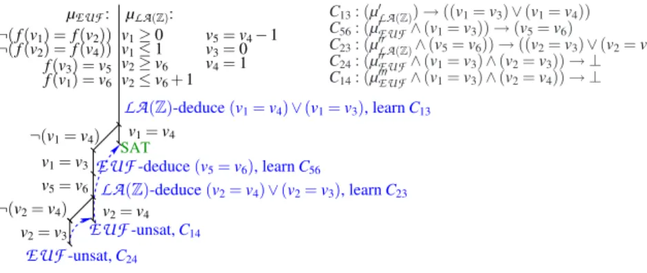
Fig. 6. DTC execution of Example 4 onLA(Z) ∪EUF, with no ei j-deduction. The clauses Ci j’s are the same as those of Fig. 8.

In the other branch of the boolean search (after the unit propagation of ¬RESET5

and (v5= v8)), since we are supposing that (v5= 0) is present in C01, then this clause

can’t be used to unit-propagate (v0= v1), and DTCstarts selecting ¬ei j’s until ¬(v0=

v1) causes again a

LA

(Q)-conflict. At this point the new clause C010 (similar to C01but

possibly involving (v5= v8) instead of (v5= 0)) is learned and (after backjumping)

(v0= v1) is unit-propagated on it. However, as a consequence of this unit-propagation,

(v3= v4) is unit-propagated on C349, and after this step DTCstarts selecting unassigned

¬ei j’s again, this time without generating conflicts, so that to conclude that the formula

is

T

1∪

T

2-satisfiable. (Comparing with the right branch in Fig. 2, we have dtc br = 2,

dtc ded = 0, no br = 1 and no ded = 2.) ¦ Notice that the three leftmost diagonal branches in Fig. 5 obtain the same effect as the ei j-deduction steps in Fig. 7 (and in Fig. 2).

As before, the fact that the DPLL solver is aware a priori of the ei j’s allows it for

learning clauses containing ei j’s, which can be used in subsequent branches in order to

prune the search and to avoid redoing the same deductions from scratch. We consider now the case where some

T

i’s are non-convex.

Example 4 (no ei j-deduction, non-convex case). Consider the

EUF

∪

LA

(Z) formula

ϕ (3) and the assignment µ of Example 2. Look at Fig. 6. Both µLA(Z)and µEUF are

found consistent in the respective theories by the respective solvers.

Then DTCstarts selecting new ¬ei j’s, and proceeds without causing conflicts, until

it selects ¬(v1= v4) and ¬(v1= v3), which cause a

LA

(Z) conflict. The branch is

in the form µ ∪S_j¬ej, so that, the ¬ei j-minimal conflict set η13 returned is in the

form µ0

LA(Z)∪ {¬(v1= v3), ¬(v1= v4)}. Thus DTC learns the corresponding clause 9_{Here we are sure that (v}

5= 0) does not appear on C34, since it was learned as a consequence of aEUF conflict.

C13(see Fig 6) and backjumps up to the highest point which allows for unit-propagating

(v1= v3) on C13, and performs such unit propagation. Then DTCstarts and proceeds

selecting new ¬ei j’s without causing conflicts, until it selects ¬(v5= v6), which causes

a

EUF

conflict represented by the clause C56. As

EUF

is convex, ¬(v5= v6) is the

only ¬ei j occurring in the conflict set, so that DTC backtracks over the last chain of ¬ei j’s and unit-propagates (v5= v6).

Again, DTCselects a chain of new ¬ei j’s without causing conflicts, until it selects ¬(v2= v4) and ¬(v2= v3), which cause a

LA

(Z) conflict represented by clause C23.

As before, it backjumps to the highest point where it can unit-propagate (v2= v3).

Performing the latter unit propagation causes a

EUF

conflict, learning the clause C24.

By applying Step 2. of Strategy 1, resolving on literals (v2= v3), (v5= v6), (v1= v3)

the conflicting clause C24 with the clauses C23, C56 and C13, (which caused the

unit-propagation of (v2= v3), (v5= v6) and (v1= v3) respectively), DTCobtains a clause

C0

24: (µ0LA(Z)∧ µ0EUF ∧ µ00LA(Z)∧ µ00EUF) → ((v1= v4) ∨ (v2= v4)), which allows it

for backjumping over all the remaining ¬ei j’s of the current chain and unit-propagating

(v2= v4).

The latter causes a new

EUF

conflict represented by the clause C14. By Step 2.

of Strategy 1, C14is resolved with the clauses C024, C13(which caused the propagation

of (v2= v4) and (v1= v3) respectively), obtaining the clause C₁₄0 : (µ0_LA(Z)∧ µ00_LA(Z)∧

µ0

EUF∧ µ00EUF∧ µ000EUF) → (v1= v4), which allows for backjumping up to µ and

unit-propagating (v1= v4).

Finally, DTCstarts and proceeds selecting ¬ei j’s (possibly unit-propagating some

value due to the clauses learned) without generating conflicts, so that to conclude that the formula is

T

1∪

T

2-satisfiable.

Comparing with Fig. 3, dtc br = 6, dtc ded = 0, no ded = 3 and no br = 3. ¦ Notice that the three leftmost diagonal branches in Fig. 6 obtain the same effect as the ei j-deduction steps in Fig. 8 (and in Fig. 3).

5 DTC with e

i j

-deduction-complete

T

i

-solvers vs. NO

In this section, we assume that both the

T

i-solvers employed by DTCare ei j-deduction

complete. Under these assumptions, we have the following result.

Theorem 2. Let

T

1and

T

2be two stably-infinite (possibly non-convex) theories and let

both

T

i-solvers be ei j-deduction complete; let ϕ be a pure

T

1∪

T

2formula and let µ

be a total assignment propositionally satisfying ϕ. Let DTCwith Strategy 1 prove the

T

1∪

T

2-consistency (resp.

T

1∪

T

2-inconsistency) of µ, returning a conflict set η in the

case of inconsistency. Let dtc br be the number of boolean branches required in the DTCproof. Then we have:

dtc br ≤ no br (5)

no br being the number of branches performed by a corresponding NO proof of the

SAT (v0= v1) EUF-unsat C67 LA(Q)-deduce (v0= v1) learn C01 C34: (µ0EUF∧ (v0= v1)) → (v3= v4) C01: (µ0_LA(Q)) → (v0= v1) C25: (µ00_LA(Q)∧ (v5= 0) ∧ (v3= v4)) → (v2= v5) C67: (µ00EUF∧ (v2= v5)) → (v6= v7) (v2= v5) RESET5 µEUF: { (v3= h(v0)), (v4= h(v1)), ¬(v6= v7), (v6= f (v2)), (v7= f (v5))} (v0= v1) (v3= v4) (v5= v8) (v5= 0) (v3= v4) ¬RESET5 EUF-deduce (v3= v4) LA(Q)-deduce (v2= v5) µ_LA(Q): {(v0≥ v1), (v0≤ v1), (v2= v3− v4)} learn C34 learn C25 LA(Q)-deduce (v0= v1) learn C0 01

Fig. 7. DTC execution of Example 5 onLA(Q) ∪EUF, with ei j-deduction-completeTi-solvers.

Theorem 2 states that, under the same hypotheses of ei j-deduction as NO, DTC

emulates NO with no extra cost in terms of boolean search.

Example 5 (convex case). Consider again the

EUF

∪

LA

(Q) formula ϕ of Example 1.

Figure 7 illustrates a DTCexecution when both

T

i-solvers are ei j-deduction complete.

On the left branch (when RESET5is selected), after the unit-propagation of (v5= 0),

the

LA

(Q) solver deduces (v0= v1), and thus by Step 4. (i) of Strategy 1, the clause

C01 is learned and (v0= v1) is unit-propagated. As a consequence of this, the

EUF

solver can deduce (v3= v4), resulting in the learning of C34and the unit-propagation of

(v3= v4), which in turn causes the

LA

(Q)-deduction of (v2= v5), with the resulting

learning of C25and unit-propagation of the deduced equality.

At this point, µ00

EUF∪{(v2= v5)}10is found

EUF

-inconsistent, so that the

EUF

-solver returns (the negation of) the clause C67, which is resolved backward with the

clauses C25, C34, C01, ¬(v6= v7), and (RESET5→ (v5= 0)) as explained in Step

2. of Strategy 1, obtaining a mixed theory+boolean conflict clause C₆₇0 in the form (µ∗∧ RESET5) → ⊥ s.t. µ∗contains no interface equality. C670 forces DTCto backjump

up to the last branching point. Then the execution of the right branch begins with the unit-propagation of ¬RESET5on C067and hence of (v5= v8) on ¬RESET5→ (v5= v8),

which produces an assignment propositionally satisfying ϕ. The theory solvers are in-voked, and the

LA

(Q) solver deduces again (v0= v1), learning a clause C010 which is

similar to C01except for the fact that it may contain the redundant literal (v5= v8)

in-stead of (v5= 0).11 Then (v3= v4) is unit-propagated on C34. At this point, since both

theory solvers cannot deduce any new ei j, by Step 5. of Strategy 1 DTCconcludes that

ϕ is

EUF

∪

LA

(Q)-satisfiable. ¦

Notice that the left branch of the DTCsearch tree of Figure 7 mimics directly that

of the NO execution of Figure 2. The main difference relies on the fact that, unlike with

10_{Hereafter, µ}0

T, µ00T, µ000T will denote generic subsets of µT,T ∈ {EUF,LA(Q),LA(Z)}. 11_{Here we assume the “worst” case in which µ}0

LA(Q) in C01 contains the (redundant) literal (v5= 0). If this is not the case, then (v0= v1) is directly unit-propagated on C01, without calling the theory solvers.

SAT f (v1) = v6 ¬( f (v1) = f (v2)) ¬( f (v2) = f (v4)) f (v3) = v5 v1≥ 0 v1≤ 1 v2≥ v6 v2≤ v6+ 1 v5= v4− 1 v3= 0 v4= 1 ¬(v1= v4) v2= v3 v1= v3 v5= v6 ¬(v2= v4) v2= v4 v1= v4 µLA(Z): µEUF: C13: (µ0LA(Z)) → ((v1= v3) ∨ (v1= v4)) C56: (µ0EUF∧ (v1= v3)) → (v5= v6) C23: (µ00_LA(Z)∧ (v5= v6)) → ((v2= v3) ∨ (v2= v4)) C24: (µ00EUF∧ (v1= v3) ∧ (v2= v3)) → ⊥ C14: (µ000EUF∧ (v1= v3) ∧ (v2= v4)) → ⊥ LA(Z)-deduce (v1= v4) ∨ (v1= v3), learn C13 EUF-unsat, C14 EUF-unsat, C24 LA(Z)-deduce (v2= v4) ∨ (v2= v3), learn C23 EUF-deduce (v5= v6), learn C56

Fig. 8. DTC execution of Ex 6 onLA(Z) ∪EUF, with ei j-deduction-completeTi-solvers.

NO, the deduced ei j’s are not exchanged directly by the

T

i-solvers, but rather they are

added to the current assignment µ and unit-propagated.

In the right branch, instead, all values are assigned directly by unit-propagation. This fact illustrates one further potential advantage of DTC with respect to NO: the fact that new ei j’s are known a priori to the DPLL engine allows their inclusion in the

learned clauses derived by theory conflicts. Thanks to unit-propagation, this makes it possible to assign truth values to them directly at the boolean level, without performing the (potentially costly) invocation of the

T

i-solvers. In the traditional NO schema, this

fact does not come naturally, because the boolean solver knows nothing about the ei j’s.

We consider now the case where some

T

i’s are non-convex.

Example 6 (non-convex case). Consider the

EUF

∪

LA

(Z) formula ϕ and assignment

µ of Example 2. Figure 8 illustrates a DTC execution when both

T

i-solvers are ei j

-deduction complete.

The first invocation of the

LA

(Z) solver results in deducing of the disjunction (v1= v4) ∨ (v1= v3) and learning of the corresponding clause C13. By Step 4.(iii)

of Strategy 1, then, (v1= v4) and (v1= v3) are put on the top of the literal

selec-tion list. As a consequence, DTCselects ¬(v1= v4), and thanks to C13 it immediately

unit-propagates (v1= v3). At this point the

EUF

solver can deduce (v5= v6), so

that the clause C56is learned and the deduced equality is unit-propagated immediately.

When µLA(Z)∪ {(v5= v6)} is passed to the

LA

(Z) solver, this deduces the disjunction

(v2= v4) ∨ (v2= v3), learning C23. Selecting ¬(v2= v4) results in the unit-propagation

of (v2= v3), which in turn causes a

EUF

conflict. After the

EUF

-solver returns

(the negation of) C24, DTC backjumps up to a point where (v2= v4) can be

unit-propagated. This results again in an

EUF

-conflict, so that the

EUF

-solver returns (the negation of) C14, which causes another backjumping up to where (v1= v4) can

be unit-propagated. Then, after another invocation to the theory solvers, DTCstops,

declaring ϕ to be

EUF

∪

LA

(Z)-satisfiable. ¦

As with the convex example, notice that the DTCsearch tree of Figure 8 mimics

6 Conclusions

Theorem 2 shows that, under the same hypotheses of ei j-deduction-completeness as

NO, DTCcan emulate NO, with no extra boolean search. Theorem 1 shows that, un-der the hypothesis of ¬ei j-minimality, even

T

i-solvers with limited or no ei j-deduction

capabilities allow DTC to emulate NO, at the cost of (at most) one extra boolean branch for every (possibly very expensive) ei j-deduction performed by NO. Both

re-sults also highlight the fact that DTCnaturally allows for learning clauses containing ei j’s, which can be used in subsequent branches to prune search and avoid redoing the

same search/deductions from scratch.

We remark that Strategy 1 has been conceived only for mimicking NO, and by no means it is assumed to be the most efficient strategy for DTC. (E.g., Step 3.(ii) can be

substituted with a weakened version of EP [4], and more efficient literal selection strate-gies might be preferable to Step 3.(i) and (iii).) Some alternatives are currently under investigation, and their theoretical properties and practical performance are subject for future work.

As far as the ¬ei j-minimality hypothesis is concerned, we notice that, at least for

theories like

EUF

and

LA

(Q), there are known decision procedures that fulfill this requirement (see [12] and [4] respectively.) For other theories, the problem of ¬ei j

-minimization opens a novel research branch.12However, we remark that DTCworks also when the

T

i-solvers are not ¬ei j-minimal, at the cost of (at most) one extra branch

to explore for each redundant ¬ei jreturned in a conflict set.

It is also important to notice that, in general, only a fraction of the assignments µ enumerated turn out to be

T

i-satisfiable for both

T

i’s, so that to require the boolean

search on the ei j’s. Thus, for all the other branches, DTCmay save the effort of many

failed attempts of deducing implied ei j’s.

On the whole, the results presented in this paper show that DTCallows for

trad-ing boolean search for ei j-deduction. Thus everyone can choose and implement the

most suitable

T

i-solvers without being forced by the ei j-deduction-completeness

strait-jacket: for theories for which efficient ei j-deduction complete procedures are available

(e.g.,

EUF

[12]), DTCallows for exploiting the full power of ei j-deduction; for harder

theories (e.g.,

LA

(Z)), the research task changes from that of finding ei j-deduction

complete

T

-solvers to that of finding ¬ei j-minimal or nearly-¬ei j-minimal ones.

References

1. A. Armando, C. Castellini, E. Giunchiglia, and M. Maratea. A SAT-based Decision Proce-dure for the Boolean Combination of Difference Constraints. In Proc. SAT’04, 2004.

2. C.L. Barrett and S. Berezin. CVC Lite: A New Implementation of the Cooperating Validity Checker. In Proc. CAV’04, volume 3114 of LNCS. Springer, 2004.

12_{Bottom line, one can always make µ ¬e}

i j-minimal by dropping the remaining ¬ei j’s one by one, each time checking µ \ {¬ei j}. Notice that, in general, with ¬ei j-minimization the search for the candidate ¬ei j’s to drop is restricted to only those occurring in µ, whilst with ei j -deduction the search for the candidate ei j’s to deduce extends to all the unassigned ei j’s.

3. M. Bozzano, R. Bruttomesso, A. Cimatti, T. Junttila, P.van Rossum, S. Ranise, and R. Sebas-tiani. Efficient Satisfiability Modulo Theories via Delayed Theory Combination. In Proc. Int. Conf. on Computer-Aided Verification, CAV 2005., volume 3576 of LNCS. Springer, 2005. 4. M. Bozzano, R. Bruttomesso, A. Cimatti, T. Junttila, P.van Rossum, S. Schulz, and R.

Se-bastiani. An incremental and Layered Procedure for the Satisfiability of Linear Arithmetic Logic. In Proc. TACAS’05, volume 3440 of LNCS. Springer, 2005.

5. M. Bozzano, R. Bruttomesso, A. Cimatti, T. Junttila, P.van Rossum, S. Schulz, and R. Sebas-tiani. MathSAT: A Tight Integration of SAT and Mathematical Decision Procedure. Journal of Automated Reasoning, 35(1-3), October 2005.

6. M. Bozzano, R. Bruttomesso, A. Cimatti, T. Junttila, P. van Rossum, S. Ranise, and R. Se-bastiani. Efficient Theory Combination via Boolean Search. Information and Computation, 204(10), 2006.

7. R. Bruttomesso, A. Cimatti, A. Franz´en, A. Griggio, and R. Sebastiani. Delayed The-ory Combination vs. Nelson-Oppen for Satisfiability Modulo Theories: a Comparative Analysis. Technical Report DIT-06-032, DIT, University of Trento, 2006. Available at http://dit.unitn.it/˜rseba/papers/lpar06 dtc extended.pdf.

8. S. Cotton, E. Asarin, O. Maler, and P. Niebert. Some Progress in Satisfiability Checking for Difference Logic. In Proc. FORMATS-FTRTFT 2004, 2004.

9. J.-C. Filliˆatre, S. Owre, H. Rueß, and N. Shankar. ICS: Integrated Canonizer and Solver. In Proc. CAV’01, volume 2102 of LNCS, pages 246–249, 2001.

10. H. Ganzinger, G. Hagen, R. Nieuwenhuis, A. Oliveras, and C. Tinelli. DPLL(T): Fast deci-sion procedures. In Proc. CAV’04, volume 3114 of LNCS, pages 175–188. Springer, 2004.

11. G. Nelson and D.C. Oppen. Simplification by Cooperating Decision Procedures. ACM Trans. on Programming Languages and Systems, 1(2):245–257, 1979.

12. R. Nieuwenhuis and A. Oliveras. Congruence Closure with Integer Offsets. In Proc. 10th LPAR, number 2850 in LNAI, pages 77–89. Springer, 2003.

13. R.E. Shostak. Deciding Combinations of Theories. Journal of the ACM, 31:1–12, 1984.

14. L. Zhang, C. F. Madigan, M. H. Moskewicz, and S. Malik. Efficient conflict driven learning in a boolean satisfiability solver. In Proc. ICCAD ’01. IEEE Press, 2001.

15. L. Zhang and S. Malik. The quest for efficient boolean satisfiability solvers. In Proc. CAV’02, number 2404 in LNCS, pages 17–36. Springer, 2002.

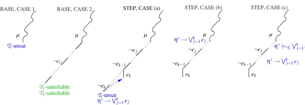
BASE, CASE 1 µ Ti-unsat BASE, CASE 2. µ ¬ei j T1-satisfiable T2-satisfiable

STEP, CASE (a)

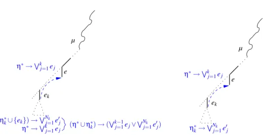
ek ¬ek ¬ek−1 ¬ej Ti-unsat η∗_→Wk j=1ej µ STEP, CASE (b) ek ¬ek−1 ¬ej µ η∗_→Wk j=1ej STEP, CASE (c) ek ¬ek−1 ¬ej µ η∗_|= Ti W_k j=1ej η∗_→Wk j=1ej

Fig. 9. Grafical representations of base cases 1. and 2. and Step cases (a), (b), (c).

A Appendix: The proofs of the theorems

Proof of Theorem 1

Proof. By induction on the structure of the DTCboolean search tree. Base: We have two basic cases (Figure 9, left).

1. Let µ be

T

i-unsatisfiable for some

T

i. The

T

i-solver detects this fact returning an

¬ei j-minimal conflict set η. Thus dtc br = 1 and dtc ded = 0. Similarly, in every

NO refutation

T

i-solver detects the

T

i-unsatisfiability of µ. Thus no ded = 0 and

no br = 1, so that (4) holds.

2. Let µ be

T

i-satisfiable for both

T

i’s, and no ei j-deduction is performed by the

T

i

-solvers. DTCselects a chain of new negated ei j’s, invoking an early-pruning check

before each new selection which cause no ei j-deduction, until no new ei j’s are

available, from which it concludes that µ is

T

1∪

T

2-satisfiable. Here dtc br = 1 and

dtc ded = 0. In every corresponding NO proof, both

T

i-solvers return “Sat” without

performing ei j-deductions (i.e., no br = 1, no ded = 0). Therefore (4) holds.

Step: If none of the previous cases holds, then DTCselects a chain of new negated

ei j’s, invoking an early-pruning check before each new selection, until either (Figure 9,

right):

(a) one early-pruning call to one

T

i-solver returns Unsat. In this case, let B denote the

current branch. The

T

i-solver returns also a ¬ei j-minimal conflict set η,

correspond-ing to the conflictcorrespond-ing clause

η∗→

k

_

j=1

ej, (6)

where ¬e1, ..., ¬ek are all the ¬ei j’s occurring in η, and η∗:= η \ {¬e1, ..., ¬ek}.

(In the corresponding NO refutation, this corresponds to the ei j-deduction µ |=Ti

W_k

j=1ej.) DTClearns the conflicting clause (6) and backjumps, popping up the

lit-erals from the branch (if k > 1) up to ¬ek−1or (if k = 1) up to the highest point in µ

where ekcan be unit-propagated on (6), and hence unit propagating ek. (In the NO

µ e ek (η∗_{∪ η}∗ k) → ( W_k−1 j=1ej∨WNj=1k e0j) (η∗ k∪ {ek}) →WNj=1k e0j η∗→Wkj=1ej η∗_→Wk j=1ej µ e ek η∗_→Wk j=1ej η∗ k→ WNk j=1e0j

Fig. 10. Graphical representation of the recursive behaviour. Case 1 (left) and 2 (right).

(b) one positive13 _e

i j, namely ek, is unit-propagated due to some previously-learned

conflict clause, which we can think w.l.o.g. in the form (6), s.t. all ¬e1, ..., ¬ej−1

and all the literals in η∗_{are in the current branch, and η}∗_{contains no negated e} i j’s.

(Notice that, in the NO refutation, this might require a novel ei j-deduction µ |=Ti W_k

j=1ej.14)

(c) One

T

i-solver performs a ei j-deduction, namely η∗|=Ti W_k

j=1ej, s.t. η∗is part of the

current branch and the ej’s are not. By Step 4. of Strategy 1, the clause (6) is learned

immediately, DTCselects in order ¬e1, ..., ¬ek−1, and hence it unit-propagates ek

on clause (6). (In the corresponding NO refutation, this corresponds to the ei j

-deduction η∗_|=

Ti W_k

j=1ejand to the selection of the branch ek.)

Let Bek:= µk∪ {ek} be the current branch, s.t. µk⊇ µ and ¬ej∈ µkfor every j < k.

Now DTCchecks recursively the

T

1∪

T

2-satisfiability of Bek.

If Bekis recursively found

T

1∪

T

2-satisfiable, then DTCconcludes that µ is

T

1∪

T

2

-satisfiable.

Otherwise, Bek is recursively found

T

1∪

T

2-unsatisfiable. By inductive hypothesis,

the DTCsub-proof requires dtc brkbranches, whilst the NO subproof requires no dedk

deductions and no brkbranches, s.t. dtc brk≤ no brk+ no dedk. Let ηkbe the conflict

set returned and let Nkbe the number of negated equalities in ηk. We distinguish two

subcases (Figure 10, left and right):

1. ek∈ ηk. Thus ηk= η∗k∪ {¬e0j}Nj=1k ∪ {ek}, s.t. η∗k does not contain ¬ei j’s. By Step

2. of Strategy 1, DTCeliminates ekfrom the conflicting clause ¬ηkby resolving it

13_{The case where one negative e}

i j is unit-propagated due to some previously-learned conflict clause C does not affect the overall discussion, because it will be eliminated from every conflict clause by means of of Step 2. in Strategy 1. No literal other than (negated) ei j’s can be unit propagated, because µ assigns a truth value to all the atomic expressions in ϕ.

14_{E.g., theEUF deduction of (v}

3= v4) in the right branch of Figure 2 corresponds to a simple unit-propagation on clause C34in Figure 5.

with (6), obtaining the new conflict clause: (η∗∪ η∗_k) → ( k−1_{_} j=1 ej∨ Nk _ j=1 e0_j). (7)

Let ¬e be the most recently assigned ¬ei j in {¬ej}k−1j=1∪ {¬e0j}Nj=1k . Then DTC

backjumps up to the highest point in Bekwhere e can be unit-propagated on (7), and

hence unit-propagates e. (Notice that (7) dominates (6) in driving the backjumping mechanism because all the ¬e0

j’s occur higher in B than ¬ek.)

2. ek6∈ ηk. Thus ηk= η∗_k∪ {¬e0j}Nj=1k , s.t. η∗kdoes not contain ¬ei j’s, corresponding to

the clause: η∗_k→ Nk _ j=1 e0_j. (8)

Let ¬e be the most recently assigned ¬ei jin {¬e0j}Nj=1k . Then DTCbackjumps up

to the highest point in Bek where e can be propagated on (8), and hence

unit-propagates e. (Notice that also (8) dominates (6) in driving the backjumping mech-anism because all the ¬e0

j’s occur higher in B than ¬ek.)

Then, DTC proceeds, each time checking recursively the

T

1∪

T

2-satisfiability on

one open branch Bej := µj∪ {ej}, each ej corresponding to either one of the original

negated ei j’s ¬e1, ..., ¬ekin B, or to one of the negated ei j’s occurring in the conflict sets

reported by the recursive sub-proofs. This is done until either a subbranch is recursively found to be

T

1∪

T

2-satisfiable, or the current dominating conflict clause forces DTC

backjumping up to a point within µ, so that µ can be declared

T

1∪

T

2-unsatisfiable, and

the negation of the dominating clause is the conflict set returned.

Let N be the number of sub-proofs performed. By inductive hypothesis, the j-th DTC sub-proof requires dtc brj branches and dtc dedj ei j-deductions, whilst the

corresponding NO sub-proof requires no dedjei j-deductions and no brj branches, s.t. dtc brj+ dtc ded ≤ no brj+ no dedj. In the cases (a)-(c) above we have respectively:

Case (a): dtc br := 1+∑N

j=1dtc brj, dtc ded := ∑Nj=1dtc dedj, no br := ∑Nj=1no brj,

and no ded := 1 + ∑N

j=1no dedj.

Case (b): no br := ∑N

j=1no brj, dtc ded := ∑Nj=1dtc dedj, dtc br := ∑Nj=1dtc brj, and

either no ded := ∑N

j=1no dedjor no ded := 1 + ∑Nj=1no dedj.

Case (c): dtc br := ∑N

j=1dtc brj, dtc ded := 1+∑Nj=1dtc dedj, no br := ∑Nj=1no brj,

and no ded := 1 + ∑N

j=1no dedj.