Alma Mater Studiorum · Universit`
a di Bologna
Scuola di Scienze
Corso di Laurea Magistrale in Fisica
SU(3) Lattice Gauge Theories and Spin
Chains
Relatore:
Chiar.ma Prof.ssa
Elisa Ercolessi
Correlatore:
Dott. Davide Vodola
Presentata da:
Costanza Benassi
Sessione I
Abstract
I modelli su reticolo con simmetrie SU(n) sono attualmente oggetto di stu-dio sia dal punto di vista sperimentale, sia dal punto di vista teorico; particolare impulso alla ricerca in questo campo `e stato dato dai recenti sviluppi in campo sperimentale per quanto riguarda la tecnica dell’intrappolamento di atomi ultra-freddi in un reticolo ottico. In questa tesi viene studiata, sia con tecniche anal-itiche sia con simulazioni numeriche, la generalizzazione del modello di Heisenberg su reticolo monodimensionale a simmetria SU(3). In particolare, viene proposto un mapping tra il modello di Heisenberg SU(3) e l’Hamiltoniana con simmetria SU(2) bilineare-biquadratica con spin 1. Vengono inoltre presentati nuovi risultati numerici ottenuti con l’algoritmo DMRG che confermano le previsioni teoriche in letteratura sul modello in esame. Infine `e proposto un approccio per la for-mulazione della funzione di partizione dell’Hamiltoniana bilineare-biquadratica a spin-1 servendosi degli stati coerenti per SU(3).
Contents
1 SU(n) groups 11
1.1 Some general properties . . . 11
1.2 SU(2) symmetry group . . . 13
1.2.1 Generators and commutation relations . . . 13
1.2.2 SU(2) and spin . . . 14
1.3 SU(3) symmetry group . . . 15
1.3.1 Generators and commutation relations . . . 15
1.3.2 SU(3) representations . . . 17
1.4 Young Tableau . . . 22
1.4.1 Young Tableau and the permutation group . . . 22
1.4.2 Young Tableau and SU(n) . . . 25
2 SU(2) Antiferromagnetic Heisenberg Model 31 2.1 An introduction to the model . . . 31
2.2 Coherent states for SU(2) . . . 32
2.3 The path integral formulation . . . 33
2.3.1 Geometrical interpretation of the Berry phase . . . 35
2.4 The continuum limit approximation . . . 36
2.5 The O(3) non-linear σ model . . . 39
2.6 A Renormalization Group transformation . . . 42
2.7 The Haldane Conjecture . . . 46
3 Theoretical and experimental approach to SU(n) systems 49 3.1 Experimental approach to SU(n) models . . . 50
3.2 Read’s and Sachdev’s approach to SU(n) systems . . . 51
3.2.1 The fermionic formulation of the SU(n) generators . . . 52
3.2.2 SU(n) coherent states . . . 53
3.2.3 The path integral formulation of the partition function . . . 54
3.2.4 CPn−1 models . . . 55
CONTENTS
4 SU(3) Antiferromagnetic Heisenberg Model 59
4.1 Two non-equivalent Hamiltonians . . . 59
4.2 A mapping into a spin-1 chain . . . 62
4.2.1 The map applied to the quantum numbers . . . 65
4.3 Numerical results . . . 68
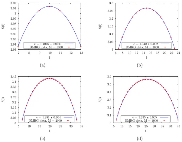
4.3.1 Numerical results for the Von Neumann Entropy . . . 70
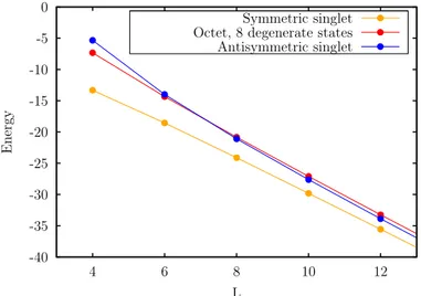
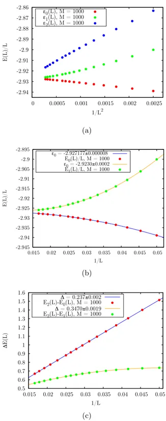
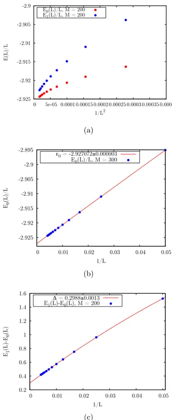
4.3.2 Numerical results for the energy spectrum . . . 72
4.4 Approach to a path integral formulation of the bilinear-biquadratic chain . . . 76
4.4.1 Coherent states for SU(3) . . . 76
4.5 The expectation value of the Hamiltonian . . . 78
A An outline of Group Theory 85 A.1 Groups and representations . . . 85
A.2 Lie groups and Lie algebras . . . 88
A.2.1 Simple Lie groups and Casimir operators . . . 91
A.3 Groups and symmetries in physics . . . 91
B An outline of DMRG 93 B.1 The density matrix . . . 93
B.1.1 Some general features . . . 93
B.1.2 Reduced density matrix and Schmidt decomposition . . . 94
B.2 Entanglement and Entropy . . . 96
B.3 The DMRG algorithm . . . 97
B.3.1 The infinite-system algorithm . . . 98
B.3.2 The finite-system algorithm . . . 99
C An outline of Conformal Field Theory 101 C.1 Conformal transformations in a 2-dimensional space . . . 101
C.2 Primary fields and Operator Product Expansion . . . 103
C.3 Radial Quantization and the Virasoro Algebra . . . 105
C.4 Some useful relations . . . 108
Introduction
SU(n) gauge theories are of fundamental importance in the description of a wide variety of physical phenomena: the interactions of a great zoology of ele-mentary particles can be described by means of those symmetries. Some well known examples are SU(3), which is the gauge-symmetry of QCD, and SU(6), which has been proposed to describe spinful quarks.
One way to extrapolate information about a lattice theory is to map it into a field theory defined on a continuous space, using a semiclassical approximation. For gauge theories, also the opposite happens, since often these theories are studied not only in the continuum, but also on a discretized lattice. In this way, it is possible to analyze gauge theories from a statistical mechanical point of view, with all the tools and techniques that statistical mechanics provides [31]. In this sense, the definition of gauge theories on a lattice constitutes a bridge between high energy physics, which requires a deep knowledge of continuous gauge theories, and condensed matter physics, whose one of main topics of interest is the study of theories defined on a discretized space. This parallelism has become recently even more important, due to the striking progresses in the field of experiments with ultracold atoms in an optical lattices [8] [24]. Trapping fermionic alkaline-earth atoms (usually some isotopes of Ytterbium or Strontium) in an optical lattice, it is possible to realize a physical system whose effective Hamiltonian presents a SU(n) symmetry. This experimental technique is very powerful since by tuning the parameters of the system it is possible to reproduce a wide variety of Hamiltonians. In this sense, these experiments may be used in order to simulate high energy phenomena on a lattice, constituting in this way a good example of quantum simulator.
From a theoretical point of view, the formalism usually used in the definition of spin chains - that is, 1-dimensional lattice models with SU(2) symmetry - can be easily generalized to SU(n) degrees of freedom, and, in this sense, it is possible to formulate SU(n) generalizations of the SU(2) quantum Hamiltonians which has been studied so much in the literature [7, 19, 22, 27]. These generalizations are based on the substitution of SU(2) generators in the explicit formulation of the Hamiltonian with the proper ones of the SU(n) group. One typical example is the
CONTENTS
case of the antiferromagnetic Heisenberg model, which has been generalized for a set of SU(n) degrees of freedom [1–3, 38, 39].
SU(2) Heisenberg model has been studied thoroughly since it is very useful in order to describe magnetic quantum systems with nearest-neighbour interactions. In the study of the path integral formulation of the partition function for the SU(2) chain, the presence of a topological term, the so called Berry Phase, is of outmost importance in order to determine the behaviour of the system. Indeed, this topological term is the one that, through the continuum limit semiclassical approximation, makes the system critical or massive depending on the value (half-integer or (half-integer) of the spin, as argued by Haldane [27]
An analogous statement holds for SU(n) antiferromagnetic Heisenberg Hamilto-nians: a topological term appears in the path integral of the partition function, and the value it takes has a great influence on the behaviour of the system. The main difference between the SU(2) and a generic SU(n) Heisenberg model is that the possible irreducible representations for SU(n) - the equivalent of the spin for SU(2) - have a reacher structure than the ones for the SU(2) case, making the semiclassical approximation more complex. In this sense, the choice of the SU(n) representation is of fundamental importance in order to determine the behaviour of the system.
The focus of this thesis is on the SU(3) generalization of the quantum antifer-romagnetic Heisenberg Model. As highlighted before, SU(3) is the gauge group of QCD. In particular, the quarks up, down and strange are organized according to the fundamental representation of SU(3), while their respective antiparticles form an antifundamental representation of the same group. In this sense, when studying a quantum “spin” Hamiltonian with SU(3) degrees of freedom on the sites of the lattice, in the fundamental or antifundamental representation, a good picture is to interpret the degrees of freedom on the chain as interacting particles (antiparticles) confined on a lattice. If we want to stick to this picture, that is, if we are interested in the fundamental and antifundamental representations of the SU(3) group, there are two possible inequivalent formulations of the Heisenberg Hamiltonian. In the first, on each site there is a particle (fundamental repres-entation), while in the second particles and antiparticles are alternated on odd and even sites respectively (so, fundamental and antifundamental representations are alternated). This, of course, changes not only the explicit formulation of the Hamiltonian, but also the quantum numbers of the system.
The SU(3) Heisenberg antiferromagnetic model with the fundamental repres-entation on the whole chain has been studied in literature; it has been shown to be critical with central charge c = 2 [2, 5], as confirmed by numerical results [5]. One interesting feature of this model is that it can be mapped into a spin-1 chain [5], the well known Lai-Sutherland model, which had already been inferred to present
Contents
a SU(3) symmetry [2]. This correspondence makes it possible to apply all the known results about the Lai-Sutherland chain to the SU(3) Hamiltonian.
As highlighted before, the choice of the representations of the SU(3) group used in the defintion of the SU(3) antiferromagnetic Heisenberg problem, is of main importance for the behaviour of the system. Indeed, if we chose to use not the fundamental representation on each site, but to alternate fundamental and antifundamental representations on odd and even sites of the chain, the physics of the system changes dramatically. A model which has been argued to have a SU(3) symmetry with alternated representations is the spin-1 biquadratic chain [14]; this system has been proved analytically to be gapped [29, 30], though its gap is so small that numerical studies on this model have often been tricky, since it could easily seem to be in a critical phase in a finite-length numerical study [11, 42].
In this work, an explicit mapping between SU(3) operators and spin-1 matrices is proposed. It makes evident the correspondence between the antiferromagnetic SU(3) Heisenberg model and spin-1 chains in both the formulation of the SU(3) Hamiltonian. Since both the Lai-Sutherland model and the biquadratic chain are particular cases of a more general spin-1 Hamiltonian depending on a parameter α, this mapping could be useful in order to study how the SU(3) symmetry ap-pears and disapap-pears varying α. In this perspective, we propose a path integral formulation of the partition function of the more general spin-1 system, formulated in terms of SU(3) generators, which could, in principle, be the starting point to find the continuum field theory underlying the spin system for any value of the parameter α.
It should be stressed that the SU(3) Heisenberg model with alternated rep-resentations has not been investigated numerically in the literature in its usual formulation, though there are many numerical works about its spin-1 analogue, the biquadratic chain [11, 14, 42]. In this work, we present some new numerical results obtained with the DMRG algorithm. Since the map we propose allows us to apply all the known results about the biquadratic spin-1 chain to the SU(3) model under study, we compare our results with the one expected from the spin-1 chain. Our estimates of the gap and of the ground-state energy are in perfect correspondence with the theoretical ones, confirming once again the equivalence between the SU(3) and the spin-1 system.
This thesis is organized as follows:
• Since our aim is to study SU(n) lattices models, an introduction to SU(n) group is given in the first chapter, with particular emphasis on SU(3), which is the group we are more interested in.
• Chapter 2 is devoted to the description of the SU(2) Heisenberg Chain; the methodology described in order to find the partition function of the model
CONTENTS
in its path integral formulation and the continuum limit turns out to be very useful, since the SU(n) Hamiltonian can be treated in an analogous way. • In Chapter 3 an introduction to the experimental and theoretical approach to
SU(n) systems is provided, in order to stress the importance of the problem and to give an highlight on the results known about this wider class of systems.
• The possibility of defining more than one non-equivalent SU(3) Heisenberg Hamiltonians is discussed in Chapter 4. The possible formulations of a SU(3)-symmetric Heisenberg Hamiltonian are described, and some highlights on their structure and feature is given. An explicit mapping between spin-1 operators and SU(3) generators is given, which allows us to apply all the known results about a wide set of spin-1 chains to SU(3)-symmetric sys-tems. New numerical results about the SU(3) antiferromagnetic Heisenberg model with alternate representations on even and odd sites are discussed. Fi-nally, an alternative approach to the path integral formulation of the SU(3) Heisenberg model is proposed and discussed.
Chapter 1
SU(n) groups
In this chapter SU(n) groups are defined and introduced [26]. Some basic gen-eral features of this class of groups is described and a notation quite common in physics is introduced. SU(2) and SU(3) are described in more detail, due to their fundamental importance in many fields of physics; for SU(3) particular import-ance is given to its representations. Moreover, when studying SU(n) groups and their representations, Young Tableau provide a powerful method to describe and catalogue representations for these groups; they will be described briefly in the last section of this chapter.
1.1
Some general properties
The SU(n) symmetry group is the group given by n× n unitary matrices with determinant equal to one. It may be shown that it is a simple Lie group (and so, it is also semisimple). It is clear that the definition itself provides a representation of the group (in terms, of course, of n × n special unitary matrices), which is called defining representation. The generators of the defining representation can be found considering that every n× n unitary matrix U can be expressed in the following form:
U = eM, (1.1.1) with M a n× n antihermitian matrix, which by definition has n2 independent
real parameters. If we require det(U ) to be equal to one, M has to be traceless because:
det(U ) = det(eM) = eTr[M ]= 1 ⇒ Tr[M ] = 0 (1.1.2) Antihermitian traceless matrices depend on n2− 1 real parameters; it means that
also U depends on the same number of parameters, which constitutes the di-mension of the Lie group, equal to the number of its generators (in each of its
SU(n) groups
representations). The Lie algebra su(n) is given by the set of n× n traceless anti-hermitian matrices. Every traceless anti-hermitian matrix can be expressed by a linear combination of the generators of SU(n), weighted by n2− 1 real parameters:
M =
n2−1
�
i=1
θiIi θi ∈ R (1.1.3)
It should be noticed that the unitary group has precisely the same generators of SU(n) plus the Identity (as we said before, U(n) is a Lie group of dimension n2);
it is only the presence or absence of the identity operator in the set of generators of the algebra that makes the difference between the unitary group and its special subgroup.
The generators of SU(n) follow the su(n) algebra (the explicit values of the structure constants depend upon the specific group):
[Ii, Ij] = cijkIk (1.1.4)
Quite often however, relation (1.1.1) is rewritten in the form - which resembles a rotation in the complex plane:
U = eiH (1.1.5)
Due to the presence of the imaginary unity at the exponential, H is an hermitian traceless matrix, still depending on n2 − 1 real parameters, so that we can write
it, analogously as in (1.1.3): H = n2−1 � i=1 θiFi θi ∈ R (1.1.6)
The Fi in (1.1.6) are a set of n2− 1 hermitian traceless n × n matrices which fulfill
the commutation relations:
[Fi, Fj] = iCijkFk (1.1.7)
It is quite common to refer to the Fi in (1.1.6) and (1.1.7) as generators of SU(n),
though this definition is slightly different from the formal one; quite analogously, we will refer to (1.1.7) as su(n) algebra, though the formal definition is given by (1.1.4).
It is worth noticing that:
1.2. SU(2) symmetry group
That is beacuse it is always possible to write a m×m unitary matrix starting from a n× n one: Um×m = � Un×n 0(m−n)×n 0n×(m−n) I(m−n)×(m−n) �
The associate m× m hermitian matrix is then in the form: Hm×m =
�
Hn×n 0(m−n)×n
0n×(m−n) 0(m−n)×(m−n)
�
1.2
SU(2) symmetry group
1.2.1
Generators and commutation relations
SU(2) is the group of 2×2 special unitary matrices. From section (1.1), we know that the numbers of the generators of SU(2) is equal to n2− 1��
n=2 = 3. The most
common choice for the generators of the defining (or fundamental) representation is:
Fi =
1
2σi i∈ {1, 2, 3} (1.2.1) In (1.2.1), σi are the well known Pauli matrices:
σ1 = � 0 1 1 0 � σ2 = � 0 −i i 0 � σ3 = � 1 0 0 −1 � (1.2.2)
The Fi matrices follow the su(2) algebra:
[Fi, Fj] = iεijkFk i, j, k ∈ {1, 2, 3} (1.2.3)
εijk is the Levi-Civita completely antisymmetric tensor. The Casimir operator of
the group for the defining representation is:
F2 = F12+ F22+ F32 (1.2.4)
By definition, it commutes with all the generators:
[F2, Fi] = 0 (1.2.5)
More generally, the Casimir operator of SU(2) may be expressed in any represent-ation as the square sum of the three generators.
SU(n) groups
1.2.2
SU(2) and spin
SU(2) symmetry group is one of the most important groups in physics, because spin degrees of freedom can be described in terms of the SU(2) group. The most simple case is the one of 12-spin, which corresponds to the fundamental represent-ation; 1
2-spin operators, up to some constants, are the Pauli matrices:
Si =
1
2�σi (1.2.6)
Of course, su(2) algebra (1.2.3) holds for these operators.
Different representations correspond to different values of the Casimir operator, that is, different values for the total square spin. The three spin operators do not commute, due to the su(2) algebra, so they can not be diagonalized at the same time; spin states are labeled by the eigenvalues of the Casimir operator S2 (labeled
with S), and of just one of the spin operators, usually S3 (labeled with s); s may
only assume values between −S and +S in steps equal to one [23]. S2|S, s� = �2S(S + 1)|S, s�
S3|S, s� = �s|S, s� (1.2.7)
Often in physics representations of SU(2) are labelled by means of spin. When calculating the direct product of SU(2) representations, the Clebsh-Gordan series describes how spin combine into different ones, for example:
� 1 2 � ⊗ � 1 2 � ={0} ⊕ {1} (1.2.8) The{0} representation corresponds to a 1-dimensional SU(2) representation, with a unique spin state|0, 0�, while the {1} representation corresponds to a 3-dimensional representation of SU(2), and so on; from a physical point of view, the global spin of a system formed by two 12-spin particle can have S = 1 or S = 0.
The SU(2) generators may also be expressed in a form which is very useful when applied to spin: S1 and S2 can be substituted by two other operators S+
and S−, defined as
S+ = S1+ iS2
S−= S1− iS2 (1.2.9)
These two operators are called ladder operators [23]; they have the following pe-culiar feature:
1.3. SU(3) symmetry group
The action of S+ and S− on a state gives the null vector in case lowering or raising
the S3 eigenvalue s makes it have a value which is not allowed in the representation
we have chosen. su(2) algebra can be written, in terms of these operators, as:
[S±, S3] = i�S±
[S+, S−] = 2�S3 (1.2.11)
In the following, when dealing with spin operators, we will consider � = 1.
1.3
SU(3) symmetry group
1.3.1
Generators and commutation relations
SU(3) is the group of 3×3 special unitary matrices; the number of its generator is equal to n2 − 1��
n=3 = 8. The most common choice for the generators in the
defining (or fundamental) representation of the group is:
Fi =
1
2λi (1.3.1)
In (1.3.1), λi are the so called Gell-Mann Matrices; their explicit formulation is:
λ1 = 0 1 01 0 0 0 0 0 λ2 = 0i −i 00 0 0 0 0 λ3 = 10 −1 00 0 0 0 0 λ4 = 0 0 10 0 0 1 0 0 λ5 = 0 00 0 −i0 i 0 0 λ6 = 0 0 00 0 1 0 1 0 λ7 = 0 00 0 −i0 0 i 0 λ8 = 1 √ 3 1 00 1 00 0 0 −2 (1.3.2) It can be easily seen how λ1, λ4 and λ6 can be obtained from σ1 - the first one of
the Pauli Matrices (1.2.2) - just shifting in the proper way its elements inside a 3×3 matrix. The same happens for λ2, λ5, λ7, which can be easily related to σ2.
λ3 and λ8 play the role of σ3, being diagonal traceless matrices.
The eight generators fulfill the su(3) algebra:
SU(n) groups
The structure constant of su(3) can be calculated [26] and their value is:
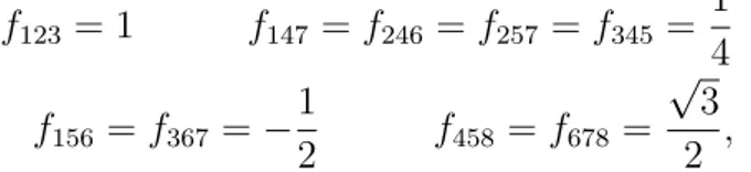
f123= 1 f147= f246= f257= f345 = 1 4 f156 = f367 =− 1 2 f458 = f678 = √ 3 2 , (1.3.4) all the others being null or obtainable by a cyclic permutation of the indices of these ones.
As SU(2) is a subgroup of SU(3), it is easy to find that particular combinations of the Gell-Mann Matrices fulfill the su(2) algebra. Let us now define a set of op-erators, which resemble in form the ladder operators usually found when studying SU(2) symmetric systems, and which will be very helpful in the study of SU(2) as subgroup of SU(3): X = X† = λ3 Y = Y†= √ 3λ8 T = λ1 2 − i λ2 2 T †= λ1 2 + i λ2 2 U = λ6 2 − i λ7 2 U†= λ6 2 + i λ7 2 V = λ4 2 + i λ5 2 V † = λ4 2 − i λ5 2 (1.3.5) The matrices (1.3.5) commute as described in table (1.1).
[X, Y ] = 0 [Y, T ] =�Y, T†�= 0 [T, U ] =−V† � T, U†�= 0 [T, V ] = U† �T, V†� � T†, U�= 0 �T†, U†�= V �T†, V� = 0 � T†, V†�=−U [U, V ] =−T† �U, V†� = 0 � U†, V� = 0 �U†, V†� = T �T, T†�=−X = −2T 3 [X, T ] =−2T �X, T†�= 2T† [X, U ] = U [Y, U ] =−3U �X, U†�=−U† �Y, U†� = 3U†
� U, U†� = X 2 − Y 2 =−2U3 [X, V ] = V [Y, V ] = 3V � X, V†�=−V† �Y, U†�=−3V† �V, V†�= X 2 + Y 2 =−2V3
Table 1.1: Commutation relations for the U , V , T operators
It must be noticed that we have chosen a notation slightly different from the usual one (in which Y = λ8, keeping the factor √13 present in the definition of
the eighth Gell-Mann Matrix, and the relations in tab.(1.1) change consequently). From (1.1) it is easy to verify that three su(2) algebras live in SU(3), having as lad-der operators U and U†, V and V†, T and T†respectively. Being ladder operators,
1.3. SU(3) symmetry group
we expect these six operators to act upon some quantum numbers, making them higher or lower; the quantum numbers we are looking for are the eigenvalues of the X and Y matrices. From (1.1), it is apparent that X and Y are two commuting operators; this means that these two matrices can be simultaneously diagonalized, and their eigenvalues are, in this sense, good quantum numbers. We will name these eigenvalues as x and y respectively, and by means of them we will label the states of the defining representation of SU(3). Indeed, it can be shown that T (T†)
lowers (raises) x by two, U (U†) raises (lowers) x by one and lowers(raises) y by three, V (V†) raises (lowers) x by one and raises (lowers) y by three. It must kept
in mind that these quantum numbers have a limited set of possible values, corres-ponding to different eigenvalues of X and Y ; when the action of a ladder operator on a state would lower or raise a quantum number to a value which is not in the set of the allowed ones, the resulting state is null, exactly as happens in the case of the ladder operators of a su(2) algebra.
From commutation relations in table (1.1), it is quite evident that the rank of the group is equal to two. Since SU(3) is a simple Lie group, Racah’s theorem states that this group is provided with two Casimir operators, which, in the fundamental representation, are: K1(F1, . . . , F8) = 8 � i=1 Fi2 (1.3.6) K2(F1, . . . , F8) = 8 � i,j,k=1 dijkFiFjFk (1.3.7)
The coefficients dijk appearing in (1.3.7) are related to the anticommutation
re-lations between Gell-Mann matrices, and may be found keeping in mind that:
{λi, λj} =
4
3δijI + 2dijkλk (1.3.8) Of course, the formulation (1.3.6) and (1.3.7) can be generalized to more complex representations of the group.
1.3.2
SU(3) representations
Before giving some explicit examples of irreducible SU(3) representations, it is useful to have some general insight of how these representations may be built. Our starting point is constituted by the U , V , and T algebras. SU(3) multiplets can be constructed from SU(2) multiplets of each of the three subalgebras U , V and T ; due to the commutation relations (1.1), these SU(2) multiplets should be coupled one to another in order to obtain a SU(3) multiplet. Moreover, being these three
SU(n) groups
su(2) algebras completely equivalent - there is no reason to prefer one to the others - we expect this symmetry to be reflected in the graphic depiction on a plane of the states of any representation (with the two cartesian axes corresponding to the eigenvalues of the generators which play the role of X and Y in that representa-tion), which should have the shape of a regular hexagon or triangle, due to the way the ladder operators act on the states and on the symmetry of their action [26].
Of course the simplest representation fulfilling all these requirements is the singlet{1}, constituted by one unique state with quantum numbers (x = 0, y = 0), as can be seen in fig.(1.1).
(0, 0)
y
x
Figure 1.1: Singlet representation of the SU(3) group
The two basic multiplet representations of SU(3) are given by the fundamental representation{3} (fig. (1.2))and the and the antifundamental one {3} (fig. (1.3)). In the case of{3}, it is apparent how the three states, which in the particle physics language are called up (u), down (d) and strange (s) respectively, are labeled by the eigenvalues of the operators X and Y : as we said before, the Fi defined
in (1.3.1) from the Gell-Mann matrices are the generators of the fundamental (defining) representation. Through the ladder operators, T (T†), U (U†) and V (V†) described in the previous section it is possible to get from one state to another
as in fig. (1.2).
The antifundamental representation is defined as the conjugate of the fun-damental one. Its generators can be found explicitly in a quite straightforward way [26]. As we have seen from (1.1.1), (1.1.2) and (1.1.6), a SU(3) transforma-tion in its defining (fundamental) representatransforma-tion, can be written as:
U = eiH, H =
8
�
a=1
θaFa, θa ∈ R (1.3.9)
Its conjugate transformation may be written as:
U = U∗ = e−iH∗ H∗ = 8 � a=1 θaFa∗, θa ∈ R (1.3.10) 18
1.3. SU(3) symmetry group T V U y x d =|2� = (−1, 1) u =|1� = (1, 1) s =|3� = (0, −2) Figure 1.2: Representation {3} ¯ T ¯ V U¯ y x ¯ d =|¯2� = (1, −1) ¯ u =|¯1� = (−1, −1) ¯ s =|¯3� = (0, 2) Figure 1.3: Representation {3} From (1.3.10) it is quite straightforward to take as generators for the antifunda-mental representation the set of matrices F = λi
2, which may be defined starting
from Gell-Mann matrices as:
λi =−λ∗i i∈ {1, ..., 8} (1.3.11)
In this new set of generators, the role of X and Y is played by
X = λ3 = −1 0 00 1 0 0 0 0 Y =√3λ8 = −10 −1 00 0 0 0 2 (1.3.12) From fig. (1.3) it is now clear that the states of the antifundamental represent-ation are labeled by the eigenvalues of X and Y , precisely as happens for the fundamental one; quite analogously, T (T†), U (U†) and V (V†) (defined as in
(1.3.5) substituting λi with λi) make it possible to shift from one state to another
as represented in fig. (1.3).
Being the fundamental and the antifundamental representations one the con-jugate of the other (the states of the {3} can be found by changing the sign of the coordinates of the ones of the {3}), often the states of the antifundamental representation are referred to as antiparticles, and are called antiup (u), antidown (d) and antistrange (s) respectively.
Irreducible representations of different dimensions are related one to the other through Clebsch-Gordan series. Some examples are:
{3} ⊗ {3} = {1} ⊕ {8}
{3} ⊗ {3} = {6} ⊕ {3} (1.3.13) In figures (1.4), (1.5), (1.6), (1.7), (1.8) some of the lowest dimensional repres-entations are depicted; x and y on the two axes represent the eigenvalues of the
SU(n) groups
d-dimensional operators that play the role of X and Y in the d-dimensional rep-resentation depicted. If there are one or more circles around a certain point of the graph, it means that there are more than one state with the same coordinates. Of course, there is no upper limit to the dimension of irreducible representations that we can find. (−2, 0) (2, 0) (−1, −3) (1,−3) (1, 3) (−1, 3) (0, 0) y x Figure 1.4: Representation {8} 20
1.3. SU(3) symmetry group (−3, 3) (−1, 3) (−1, 3) (1, 3) (3, 3) (1,−3) (−2, 0) (2, 0) (0,−6) (0, 0) y x 1 Figure 1.5: Representation {10} (3,−3) (−2, 0) (2, 0) (1, 3) (1,−3) (−1, −3) (−3, −3) (−1, 3) (0, 6) (0, 0) y x 1 Figure 1.6: Representation {10} (−2, −2) (2,−2) (−1, 1) (1, 1) (0, 4) (0,−2) (2, 4) (−2, 4) (−3, 1) (3, 1) (−1, −5) (1,−5) y x Figure 1.7: Representation {15} (2, 2) (−2, 2) (1,−1) (−1, −1) (0,−4) (0, 2) (−2, −4) (2,−4) (3,−1) (−3, −1) (1, 5) (−1, 5) y x Figure 1.8: Representation {15} 21
SU(n) groups
1.4
Young Tableau
Young tableau are a useful and powerful method to describe different repres-entations of the permutation group Sn and of SU(n) through a graphic depiction
in accordance with a set of simple rules. Though they were born in the context of the study of permutations, they can be transposed also to the case of SU(n); since they are so easy to use and interpret,Young diagrams give us one efficient tool to manipulate SU(n) representation. In this section, Young tableau will be described both in the context of Sn and SU(n) [26]; for the SU(n) case particular
stress will be put on the method for the evaluation of direct products between representations [26].
1.4.1
Young Tableau and the permutation group
Given a set of n objects (particles, numbers, . . . ) a permutation is a trans-formation of the set which interchanges some (or all) objects of the set between themselves. If only two objects are exchanged one with the other, the permutation is called transposition; we can define a transposition operator Pij, which exchanges
the i-th object with the j-th one. Every permutation can be obtained by a combin-ation (product) of transpositions; the way this combincombin-ation may be defined is not unique, but every possible set of transposition by which we can obtain a certain permutation is formed by an odd or even number of transpositions. Thanks to this property, it is possible to define a sign for the permutation, which is equal to 1 if the permutation is even or−1 if it is odd. The set of all possible permutations of n objects is a group, and it is called permutation group Sn: indeed, it is quite evident
that, once we have defined the identity element I which leaves the set unaltered, all the requirements necessary to define a group, stated in section (A.1), hold.
An explicit physical formulation may be useful to visualize the permutation group. Let us define a two-particles wave function ψ(1, 2), which will be a function of all the degrees of freedom of the two identical particle; with the numbers 1, 2, . . . we denote the whole set of degrees of freedom. The transposition operator P12
will act on this state in the following way:
P12ψ(1, 2) = ψ(2, 1) (1.4.1)
In (1.4.1), we have exchanged the two particles or, equivalently, the first particle has assumed all the degrees of freedom that were of the second, and viceversa. It is possible to define a symmetric and an antisymmetric (under exchange of the degrees of freedom) wave function (ψs, ψa):
1.4. Young Tableau
It is easy to verify that these two wave function are really symmetric or antisym-metric:
P12ψs = ψs P12ψa=−ψa (1.4.3)
Of course, it is possible to define symmetric or antisymmetric wave functions with an arbitrary number of particles, and given a generic wave function ψ(1, 2, ..., n) through a proper set of transpositions we can symmetrize or antisymmetrize it.
Let us now define what a Young tableaux (or Young diagram) is using as example the states in (1.4.2) We denote with a column of m boxes a state which is completely antisymmetric under the exchange of m indices, while a column with nc row will represent a state which is completely symmetric under the exchange of
nc indices. The two two-particles wave functions (1.4.2) are then represented by:
ψs= ψa = (1.4.4)
Of course, this notation can be generalized to any number of particles, but with a caveat: the number of boxes should always be equal to the number of particles. There are also more complicated cases than the one of completely (anti)symmetrized wave functions, because it is possible to have mixed symmetry states, which are (anti)symmetric only under the exchange of some particles and only in a certain number. For example, for three particle states, there are three possible cases:
ψs = ψmix= ψa = (1.4.5)
In (1.4.5) ψmix is a state symmetric under exchange of two of the three particles,
and antisymmetric under the exchange of one of these two with the third. It should be noticed that, no matter how many particles we are considering, the completely symmetric and the completely antisymmetric states are unique: there is just one way to symmetrize or antisymmetrize completely a state. To have all the possible states which fulfill a certain n-particles (mixed) symmetry, it is enough to take the correspondent Young Tableaux and to fill it with all possible numbers from 1 to n, taking into consideration also the combinations with repeated numbers, but sticking to the following requirements - which describe the so called standard form for a Young diagram:
• The numbers must not decrease along a row, from left to right; • The numbers must increase along a column, from top to bottom;
SU(n) groups
• The number of boxes in a column must not be lower than the number of boxes in the following one, from left to right.
It should be noticed that if we stick to these requirements properly, we do not have all the possible states. For example, for three-particles wave function, these two states are allowed:
1 2 3
1 3
2 (1.4.6)
These ones, however, are not:
1 2 3
1 3
2 (1.4.7)
They describe a wave function symmetric under the exchange of particles 1 and 2 and antisymmetric under exchange of particles 2 and 3, and symmetric under the exchange of particles 1 and 3 and antisymmetric under exchange of 3 and 2, respectively. However, these two states can be obtained by using the group operators Pij on the two states (1.4.6) respectively: we have found two invariant
subspaces of S3. In this sense, the standard form of Young tableau lets us catalogue
all irreducible representations of Sn through all the possible allowed combinations
of n boxes. When we fill the boxes of a certain diagram in all the proper ways with numbers from 1 to n, we get a series of states which form a basis for an irreducible representation of the group characterized by certain (anti)symmetry properties, though we should also consider configurations of the diagram which are not allowed in order to have all the states of the representation: the number of possible allowed ways we can fill a given tableaux is equal to the dimension of the correspondent representation.
Given a permutation group Sn, it is possible to catalogue all its Young diagrams
through a set of numbers qi, each of them corresponding to the number of boxes in
the i-th row; for example, the tableau for S3(1.4.5) may be characterized as (3,0,0),
(2,1,0), (1,1,1) respectively. Another way to characterize the Yang tableaux of Sn
is using not qi, but another set pi defined as pi = qi− qi+1. States (1.4.5) may then
be described by (3,0,0), (1,1,0), (0,0,1).
It is possible to define the conjugate Young diagram of a given one: each row becomes a column and each column becomes a row. It is clear that the dimensions of the representations related to a Young tableaux and to its conjugate one are the same: conjugate diagrams correspond to different representations with the same
1.4. Young Tableau
dimension. To exemplify, let us consider the four possible representations of S4:
(1.4.8)
The conjugation relations for these Young Tableau are:
⇐⇒
⇐⇒
⇐⇒ (1.4.9)
The completely symmetric and the completely antisymmetric states are one the conjugate of the other; moreover, we can see that the last diagram in (1.4.9) is self-conjugate.
1.4.2
Young Tableau and SU(n)
In the previous paragraph, we have seen how Young diagrams work in the case of the permutation group SN. Quite an analogous treatment may be applied to
the case of SU(n), on the basis of the following theorem: every state formed by N particles, belonging to the permutation group SN and generated by composing
single-particle states of a n-dimensional SU(n) multiplet belongs also to an irredu-cible representation of SU(n) [26]. This theorem has a series of consequences; firs of all, it means that we can apply the Young tableau method to SU(n), keeping in mind that a diagram representing a SU(n) multiplet may have columns with a maximum of n boxes - that is, we can have a maximum of n rows. The reason is quite clear: if we have a state formed by particles of a n-dimensional multiplet, it makes no sense to try to antisymmetrize a state with n + 1 particles. Moreover, since the completely antisymmetric state is uniquely defined, columns with exactly n boxes may be omitted, because they do not contribute to the dimension of the
SU(n) groups
irreducible representation of SU(n) we are describing by means of the diagram. For example, let us consider SU(3): in (1.4.10) we see how a state with three-boxes columns may be reduced to an equivalent one.
=⇒ (1.4.10)
In this formulation, every tableaux represents an irreducible representation of SU(n), whose dimension will be equal to the numbers of way to fill the N boxes of the diagram with the numbers from 1 to n in a standard configuration; in this sense, every box will correspond to a particle, and the number inside it labels the state the particle is in.
We will call fundamental representations of SU(n) the representations related to Young tableau with only one of the pi different from zero. The fundamental
representations for SU(2), SU(3), SU(4) are:
SU(2) : (1.4.11)
SU(3) : (1.4.12)
SU(4) : (1.4.13)
For the SU(3) case (1.4.12), these two representations are the ones that in section (1.3.2) we called fundamental and antifundamental respectively.
In the case of SU(n), we can define the conjugate of a Young diagram in a slightly different way than what we did for the permutation group. Let us consider a diagram characterized by a set of integers number pi as defined in the previous
section; its conjugate representation is the one with the same set pibut in opposite
order, that is:
(p1, ..., pn−1) =⇒ (pn−1, ..., p1) (1.4.14)
One simple example of conjugation is:
1.4. Young Tableau
From the comparison of (1.4.9) and (1.4.15) it is quite evident that the definition of conjugation we have given when studying the permutation group and the one considered for the SU(n) case are not equivalent at all.
As our main interest is in the SU(3) symmetry group, let us now introduce the Young tableau for some of its representations. First of all, there are the fundamental and antifundamental representations (1.4.12); it is clear that they are one the conjugate of the other. For the octet representation we will have the diagram:
{8} (1.4.16) This tableaux may be filled, as we expect, in eight different ways according to a standard configuration: 1 1 2 1 1 3 1 2 2 1 2 3 1 3 2 1 3 3 2 2 3 2 4 3 (1.4.17) The other three-boxes tableau we may have for a SU(3) symmetry are:
{10} (1.4.18)
≡
①
{1} (1.4.19)It is not difficult to verify that (1.4.18) and (1.4.19) have dimensions equal to 10 and 1 respectively (for (1.4.19) it is due to the fact that for a SU(3) symmetry we can omit columns with 3 boxes).
It is clear that, for more complex representations, it may be exceedingly long to calculate how many standard configurations are possible for a given tableaux. What we need is a general formula allowing us to calculate the dimension of a diagram in a quicker way. Firstly, let us notice that for a representation of SU(n + 1), only n integers{p1, ..., pn} are needed to characterize its tableaux, since columns
with n + 1 boxes may be omitted. When we want to study the same diagram in the context of SU(n), all that we need to do is to eliminate the last pi, that is, all
columns with n boxes: in SU(n) the same diagram is defined by a set{p1, ..., pn−1}.
A recursion formula may be proved, on the basis of these considerations; if we denote with Dn(p1, ..., pn−1) the dimension of the tableaux represented by the set
(p1, ..., pn−1) interpreted as diagram for SU(n), we have:
Dn+1(p1, ..., pn) =
1
n!(pn+ 1)(pn+ pn−1+ 2)...(pn+ ... + p1+ n)Dn(p1, ..., pn−1) (1.4.20)
SU(n) groups
Thanks to (1.4.20) it is possible to calculate the dimension of a Young tableaux (that is, an irreducible representation) in SU(n + 1) using the knowledge of the dimension of the same diagram in SU(n).
This formula may well be simplified for the case of SU(3). First of all, let us notice that the only possible diagrams for SU(2) are the ones with just one row of p1 boxes. Since we can fill the boxes only with 1s and 2s, the diagrams in a
standard form will have a set of numbers 1 followed by a set of numbers 2. There are exactly (p1+ 1) configurations of this type: the one with just numbers 1 and
no numbers 2, and p1 configurations, in which the number two is repeated from a
certain box to the end of the row:
1 1 1 . . . . . . 1 1 1 � 1 configuration 1 1 1 . . . . . . 1 1 2 1 1 1 . . . . . . 1 2 2 ... 2 2 2 . . . . . . 2 2 2 p1 configurations
We can then arrive to the conclusion that:
D2(p1) = p1+ 1 (1.4.21)
Thanks to (1.4.21) it is possible to apply (1.4.20) to the SU(n) case, in particular also to the SU(3) one. What we find is:
D3(p1, p2) =
1
2(p2+ 1)(p1+ p2+ 2)D2(p1) = 1
2(p2+ 1)(p1+ p2+ 2)(p1+ 1) (1.4.22) This formula gives us a simple way to calculate the dimension of the representation of SU(3) related to a given Young tableaux.
It is worth stressing that, in the context of SU(3), the two integer numbers p1
and p2 characterizing a representation may be also used to evaluate the Casimir
operator K1 defined in (1.3.6) for that representation: it can be shown that the
following relation holds:
K1 =
p2
1+ p22 + p1p2
3 + p1+ p2 (1.4.23) (1.4.23) provides a simple way to calculate one of the Casimir operators of SU(3), which helps us to recognize different multiplet representations of the group.
We now turn to the description of how Young diagrams may be used to evaluate direct products: Young tableau provide indeed a powerful and efficient method to
1.4. Young Tableau
find the direct product between representations of SU(n), and so to calculate the related Clebsch-Gordan series. Let us consider two Young tableau for two represen-tations of SU(n), for example two octets of SU(3), and let us study their inner product:
⊗ ={8} ⊗ {8} (1.4.24) The idea is to label all the boxes of the second representation with letters{a, b, . . . }, giving the same label to boxes in the same row in increasing order from top to bottom of the diagram, and then to juxtapose the boxes of the second tableaux to the first tableaux in all possible ways in order to obtain new Young diagrams with the following constraints:
• The new tableaux must be in a standard form; • There must be no columns with more than n boxes;
• The letters of the alphabet {a, b, . . . } in the boxes from the second diagram must increase from top to bottom of a column;
• The letters of the alphabet {a, b, . . . } in the boxes from the second diagram must not decrease from left to right of a row;
• If we count from right to left of each row of the new tableau, as we go down from top to bottom of the diagram, the number of times the (k + 1)-th letter has been repeated must never exceed the number of repetition of the k-th one;
For example, in the case (1.4.24), we get:
⊗ a a b = a a b ⊕ a a b ⊕ a a b ⊕ a a b ⊕ a a b ⊕ b a a = ⊕ ⊕ ⊕ ⊕
①
⊕ (1.4.25) {8} ⊗ {8} = {27} ⊕ {10} ⊕ {10} ⊕ {8} ⊕ {1} ⊕ {8} (1.4.26)Chapter 2
SU(2) Antiferromagnetic
Heisenberg Model
This chapter is devoted to the study of the Antiferromagnetic Heisenberg Model and of its behaviour. Firstly, the model is defined and its Hamiltonian formulated; secondly coherent states for the SU(2) symmetry group are introduced [7, 35]. We then turn to the study of the path integral formulation for the partition function [7, 22]. The discrete system under analysis can be mapped into a continuous one, under a continuum limit [19,22], and the continuous model we find is described [37]. The well known Haldane Conjecture [27] is formulated and described through a Renormalization Group transformation [22, 34].
2.1
An introduction to the model
Let us consider a chain, that is, a 1-dimensional lattice, with constant lattice spacing a. On each site of the chain we suppose that there is a single particle with a certain quantum spin S, and that only the spin degree of freedom of the particles matters in the definition of our system. The simplest interaction between particles on a spin chain is a nearest-neighbour interaction, that is, a two-body interaction between particles situated on sites one next to the other. One of the most important models for a spin chain of this kind is the Heisenberg model, whose Hamiltonian is:
ˆ
H = J�
i
Si· Si+1 (2.1.1)
Si denotes the spin operators acting on the i-th site of the chain; the Hamiltonian
can be formulated as: ˆ
H = J�
i
�
S1iS1i+1+ S2iS2i+1+ S3iS3i+1
�
SU(2) Antiferromagnetic Heisenberg Model
It is clear that this hamiltonian is isotropic along each of the three axes. Of course, it can be generalized, for example, assuming some kind of anisotropy or introducing an external magnetic field; in the following we will consider only the simple formulation (2.1.1).
Another characteristic that is very important for the behaviour of this physical system is the sign of the coupling constant J: if J > 0 the model is antiferro-magnetic, if J < 0 it is ferromagnetic. Depending on the sign of J, the states of the spectrum dispose themselves differently: if the chain is ferromagnetic, the lowest energy states are the one with a ferromagnetic order, that is with the spins aligned, while in the antiferromagnetic case states with a Neel order, that is, with a staggered disposition of the spins on the chain, are favoured. Changing the sign of J, the lowest energy states become the most excited and viceversa. Moreover, it should be noticed that, depending on the value S of the spin on each site, the Si constitute a different representation of the SU(2) group on each site; the Young
diagram of a representation of given S is a row of 2S boxes: . . .
. . .
� �� �
2S boxes
(2.1.3)
We are interested in the case of an Heisenberg Antiferromagnetic SU(2) spin chain, with a S-spin particle on each site. Our starting point is the partition function of the model, which determines the thermodynamic behaviour of the system:
Z = Tr�e−β ˆH� (2.1.4) This quantity will be studied thoroughly in the following using a path integral formulation; to define a path integral, the so called coherent states will be needed. The next section is devoted to the introduction and the description of this set of states and of its properties.
2.2
Coherent states for SU(2)
It is a result of group theory [7] that every operator G of the SU(2) S-spin representation can be expressed as:
G = eiφS3eiθS2eiχS3 (2.2.1)
θ, φ and χ determine univocally the matrix G. Their range is θ∈ [0, π], φ ∈ [0, 2π[, χ∈ [0, 2π[. The set of coherent states can be found applying the operator (2.2.1) to the highest weight state, that is, for SU(2), the maximally polarized state |S, S�; since in quantum mechanics states are defined up to a phase, χ can be
2.3. The path integral formulation
fixed arbitrarly. The coherent state |Ω� can be parametrized by a classical three-dimensional real unimodular vector Ω = (Ω1, Ω2, Ω3), with:
Ωi =
1 S�Ω|S
i|Ω� (2.2.2)
The explicit expression for Ω is:
Ω =�sin(θ) cos(φ), sin(θ) sin(φ), cos(θ)� (2.2.3) It should be noticed that (2.2.3) does not depend upon χ, as expected: two angles are enough to define the coherent states for SU(2). It can be proved [7] that the set of states |Ω�, depending on θ and φ, are overcomplete; the resolution of the identity is: 2S + 1 4π � dΩ|Ω��Ω| = 2S + 1 4π � dφdθ sin(θ)|Ω��Ω| = I (2.2.4) It can be easily verified that the quantum state |Ω� is normalized to one.
A many-particle coherent state, as the ones we will consider in the following, may be defined as:
|Ω� = ⊗i|Ωi� (2.2.5)
In (2.2.5), |Ωi� denotes the single-particle coherent states of each of the particle
contributing to the final state, each one depending on its angles θi, φi and χi. The
resolution of the identity (2.2.4) can be easily generalized for a set of many-particles coherent states.
2.3
The path integral formulation
Let us now go back to the partition function (2.3.13); the first step of our analysis is to formulate this quantity by means of a path integral [7, 22]. To do so, it is useful to notice that:
Z = Tr�e−β ˆH� = lim N→∞Tr �� e−NβHˆ �N� (2.3.1)
In (2.3.1) we have only divided β in N intervals and taken the limit for N → ∞. The trace can be expressed in a more explicit way through the coherent states of our system at temperature β:
Z = lim N→∞ � �� i dΩi(β) � �Ω(β)|�e−NβHˆ �N |Ω(β)� (2.3.2)
SU(2) Antiferromagnetic Heisenberg Model
Let us now introduce N resolutions of the identity, and, ignoring constant factors preceding Z, we find: Z = lim N→∞ � �� i,τ dΩi(τ ) � β � τ =� �Ω(τ + �)|e−� ˆH(τ )|Ω(τ)� (2.3.3)
In (2.3.2) � = Nβ, τ is an integer multiple of � and we are assuming|Ω(β)� = |Ω(0)�. Since � can be regarded as a very small quantity, we can now proceed to a Taylor expansion of the exponential to the first order in �:
Z = lim N→∞ � �� i,τ dΩi(τ ) � β � τ =� �Ω(τ + �)|(1 − � ˆH)|Ω(τ)�) (2.3.4) It is now convenient to define the classical hamiltonian H as a normalized expect-ation value of the operator ˆH:
H(τ ) = �Ω(τ + �)| ˆH|Ω(τ)�
�Ω(τ + �)|Ω(τ)� (2.3.5) Substituting (2.3.5) in (2.3.4), and exponentiating the hamiltonian again it is easy to obtain: Z = lim N→∞ � �� i,τ dΩi(τ ) � β � τ =� e−�H(τ)�Ω(τ + �)|Ω(τ)� = lim N→∞ � �� i,τ dΩi(τ ) � β � τ =� e−�H(τ)(1 + �� ˙Ω(τ)|Ω(τ)�) = lim N→∞ � �� i,τ dΩi(τ ) � β � τ =� e−�H(τ)+�� ˙Ω(τ)|Ω(τ)� (2.3.6)
We now have to evaluate the scalar product� ˙Ω(τ)|Ω(τ)�; it can be shown that the following result holds for the coherent states we defined in section (2.2) [7]:
� ˙Ω(τ)|Ω(τ)� =� j � ˙Ωj(τ )|Ωj(τ )� = � j i ˙φjcos(θj) (2.3.7)
Moreover, also the hamiltonian H can be evaluated; keeping in mind that the quantum hamiltonian ˆH is (2.1.1), H is defined as (2.3.5) and that (2.2.3) holds, it is quite straightforward to find, at the zeroth order in �:
H(τ ) = JS2�
i
2.3. The path integral formulation
We now have all we need to turn to a path integral formulation of the partition function. First of all, we define an integration measure for our integral:
DΩ = lim
N→∞
�
i,τ
dΩi(τ ) (2.3.9)
Since � is vanishing small, we can consider τ as a continuous variable; the final expression we find keeping in mind all we have done so far is:
Z = � DΩ e−�0βdτ H(τ )+iS � iω(Ωi) (2.3.10) ω(Ωi) = − � β 0 dτ ˙φi(τ ) cos(θi(τ )) (2.3.11)
The term S�iω(Ωi) is called Berry phase, and will contribute in a fundamental
way to the description of the model, since it will give some topological information about it. Of course, formulation (2.3.11) may be summarized as:
Z = � DΩ e−S(Ω) (2.3.12) S = � β 0 dτ H(τ )− iS� i ω(Ωi) (2.3.13)
S is the action for our model, which will be of great importance in the following for the understanding of the behaviour of this system. Of course, this procedure can be done precisely in the same way for any other spin-model, substituting ˆH with the appropriate quantum hamiltonian.
2.3.1
Geometrical interpretation of the Berry phase
The Berry phase is not explainable in terms of the Hamiltonian of our system: its form is due to the structure of the coherent states, and a geometrical interpret-ation of this quantity by means of the classical spin vectors Ωi(τ ) can be given [7].
Each one of the Ωi(τ ) is bounded, by its own nature of unimodular vector, to
move upon a spherical surface of unitary radius; at any change of τ it changes direction, but not lenght, describing a trajectory upon this sphere, which can be parametrized using the parameter τ . In this picture, of course the angles θ(τ )i
and φ(τ )i constitute the latitude and the longitude respectively of the points on
the sphere belonging to the trajectory. Since |Ω(β)� = |Ω(0)� the trajectories on the sphere are closed ones; this implies that it is possible to express ω(Ωi) of the
Berry phase in an equivalent formulation:
ω(Ωi) =− � β 0 dτ ˙φi(τ ) cos(θi(τ )) = � β 0 dτ�1− ˙φi(τ ) cos(θi(τ )) � (2.3.14)
SU(2) Antiferromagnetic Heisenberg Model
(2.3.14) can be easily recognized as the area on the spherical surface enclosed by the trajectory described by Ωi(τ ). It is then possible to use Stoke’s theorem, and
to express ω(Ωi) as [7]: ω(Ωi) = � β 0 dτ Ai(Ωi)· ˙Ωi ∇ × Ai· Ωi = 1 (2.3.15)
Aiis a vector potential, similar to the one usually defined in the context of classical
electromagnetism. Of course, there is a gauge freedom in the choice of Ai, and
many equivalent formulations are possible for it.
2.4
The continuum limit approximation
The Heisenberg model, being defined on a lattice, describes the 1-d space as discrete; what we would like to do now is to study the continuum limit approx-imation of this model, in which space is treated as continuous. In order to do so, we shall consider a semiclassical approximation, which holds only in the large-S limit [7, 19, 22]. Firstly, we express the classical spin vector Ωi(τ ) through the so
called Haldane Ansatz:
Ωi = (−1)imi � 1− a 2 S2li· li+ a Sli (2.4.1) In (2.4.1), mi is called N´eel field, and constitutes the slowly varying part of the
classical vector; its norm is equal to one, precisely as Ωi, and it keeps track of the
staggered N´eel order which is favoured by the antiferromagnetic coupling through the term (−1)i, which gives a different sign on odd and even sites. l
i is the canting
field, and it is supposed to be very small: it constitute a correction to the main term constituted by mi, to which it is orthogonal. These two fields have then the
following properties:
mi· mi = 1 mi· li = 0 (2.4.2)
In the continuum limit, the lattice constant a becomes vanishing small, and sums over the sites are replaced by integration over a continuous space variable x. mi becomes then m(x), and li becomes l(x); we are allowed to have a Taylor
expansion for mi+1 and for Sali+1 to the second order in a:
mi+1 = m(x) + a ∂m(x) ∂x + 1 2a 2∂2m(x) ∂x2 a Sli+1 = a Sl(x) + a2 S ∂l(x) ∂x (2.4.3)
2.4. The continuum limit approximation
Moreover, due to (2.4.2), it is clear that
m· ∂m
∂x = 0 (2.4.4)
The continuum limit Hamiltonian is found taking (2.4.3) and (2.4.4) into con-sideration, and Taylor expanding to the second order in a: since the classical Hamiltonian is in the form (2.3.8), one gets - ignoring constant factors - [19]:
� β 0 dτ H(τ ) = J � β 0 dτ dx � −a 2m· ∂2m ∂x2 + 2 a S2l(x)· l � (2.4.5)
After an integration by parts, we find the final form for the continuum limit of the Heisenberg Hamiltonian: � β 0 dτ H(τ ) = � β 0 dτ dxJa 2 � S2∂m ∂x · ∂m ∂x + 4l· l � (2.4.6)
Let us now turn to the Berry phase (2.3.11): to have the continuum form for the effective action S (2.3.13), it also has to be formulated for a continuous 1-dimensional space, as we have just done for the hamiltonian. Though it will be trickier from an analytical point of view, the idea is exactly the same: to substitute the Haldane Ansatz (2.4.1) for Ωi in the Berry phase and to evaluate it
consequentely. First of all we notice that, since li is the small rapidly varying part
of the Haldane Ansatz, and plays the role of a correction, one is allowed decompose Ωi as: Ωi = Λi+ δΛi Λi = (−1)imi δΛi = a Sli (2.4.7)
In the previous expression, Λi is the dominating part of the field, that is, the one
depending on mi in the Haldane Ansatz (2.4.1) (we have regarded the square root
term as negligible, since li is a small fluctuation), and δΛi is the correcting term
depending only on li; consequentely, it is possible to write:
ω(Ωi) = ω(Λi) + δω(δΛi) (2.4.8)
To evaluate δω(δΛi), it is better to use the formulation (2.3.15) of the Berry phase,
which uses a vector potential Ai; after some algebra [19], one can find that the
variation of ω is: δω(Λi) = � β 0 dτ δΛi· � Λi× ∂Λi ∂τ � (2.4.9)
SU(2) Antiferromagnetic Heisenberg Model
Substituting (2.4.7) in this expression, we find:
δω(li) = a S � β 0 dτ li· � mi× ∂mi ∂τ � (2.4.10)
Let us now formulate the Berry phase in the continuum approximation:
S� i ω(Ωi) = Γ(m) + � dxdτ l· � m×∂m ∂τ � (2.4.11)
Γ(m) is the continuum limit for S�iω(Λi). To calculate it, it is important to
keep in mind the staggering factor (−1)i in (2.4.7):
S� i ω(Λi) = S � i (−1)iω(mi) = S � i (ω(m2i)− ω(m2i+1)) (2.4.12)
Expanding in a Taylor series, keeping only the first derivative of m, one finds, turning to the continuum expression [7, 19]:
Γ(m) = S 2 � dxδω δm · ∂m ∂x = S 2 � dx � mi× ∂mi ∂τ � · ∂m(x) ∂x = ϑ 4π � dxdτ � ∂m ∂τ × ∂m ∂x � · m (2.4.13) ϑ = 2πS (2.4.14)
Getting all we did so far together, the actionS has the form:
S = S1 +S2 (2.4.15) S1 = � dxdτJa 2 � S2∂m ∂x · ∂m ∂x + 4l· l � − i � dxdτ � m× ∂m ∂τ · l � (2.4.16) S2 = −iΓ(m) (2.4.17)
Let us keep in mind that our partition function is in now in the form:
Z = �
2.5. The O(3) non-linear σ model
Our final step is to perform the integration of the rapidly varying variable l; in order to do so, it is enough to notice that S1 can be rearranged in order to make
it possible a gaussian integration, just completing the square:
2aJl·l−im×∂m ∂τ ·l = �√ 2Jal− i m 2√2Ja × ∂m ∂τ �2 + 1 8Ja � m× ∂m ∂τ �2 (2.4.19)
We can now integrate the l variable of our path integral - which will give only a constant multiplicative factor before Z, that can be ignored -. Let us notice that:
m· ∂m ∂τ = 0 ⇒ � m×∂m ∂τ �2 = ∂m ∂τ · ∂m ∂τ (2.4.20) The path integral we have is then [7, 19, 22]:
Z = � Dm δ(m· m − 1)e− ˜S−iΓ(m) (2.4.21) ˜ S = � dxdτ ˜L (2.4.22) ˜ L = 1 2g � v � ∂m ∂x �2 + 1 v � ∂m ∂τ �2� (2.4.23) g = 2 S v = 2Jsa (2.4.24) The Lagrangian (2.4.23) can be recognized as the one of the so called O(3) non-linear σ model (NLσM) in its euclidean formulation; this gives us an hint of what is the physical interpretation of the procedure described so far. What we have now is a path integral of the exponential of the action of a field theory in its euclidean formulation: this object corresponds to the euclidean (Wick-rotated) generating functional for the field theory found through the continuum limit, evaluated with no external sources. We have then taken advantage of the correspondence between quantum statistical mechanics and quantum field theory, mapping the original spin chain in one dimension into a field theory in 1+1 dimensions (the role of time is played by the temperature τ ) with well known characteristics.
The next section will provide an outline of the features of the classical O(3)NLσM and of its most important topological properties [37].
2.5
The O(3) non-linear σ model
The O(3) non-linear σ model describes three free real scalar fields (m1, m2,
SU(2) Antiferromagnetic Heisenberg Model
vector field m(x, τ ) is supposed to have modulus equal to one at any point of our 2-dimensional space-time: m(x, τ ) = mm12(x, τ )(x, τ ) m3(x, τ ) m(x, τ )· m(x, τ) = 3 � i=1 (mi(x, τ ))2 = 1 (2.5.1)
Due to constraint (2.5.1), m can vary only on a sphere: this two-dimensional spheric surface constitutes an internal space for the possible configurations of the vector field, which must not be confused with the 1+1 dimensional space in which the fields mi live.
The Lagrangian has the following form [37]:
L = 1 2 2 � µ=1 3 � i=1 ∂mi ∂xµ ∂mi ∂xµ = 1 2 2 � µ=1 ∂m ∂xµ · ∂m ∂xµ (2.5.2)
In (2.5.2), x1 = x, x2 = τ and Lorentz convention for up and down indices is used.
In order to find the equation of motion, we should minimize the action, imposing that it encodes the constraint (2.5.1) by means of a Lagrange multiplier:
S = �
dxdτ (L(x, τ) − λ(x, τ) (m · m − 1)) (2.5.3) The equation of motion is then:
(� + λ)m = 0 (2.5.4) It can be further simplified using the constraint (2.5.1):
m· (� + λ)m = 0 ⇒ λ = −m · �m ⇒ (� − m · �m) m = 0 (2.5.5) If we do not want to take into account the time dependence of the solutions of the equation of motion, but only to consider the static set of solutions, we can formulate the static equation of motion as:
� ∂2 ∂x2 − � m·∂ 2m ∂x2 �� m = 0 (2.5.6)
Of course it is possible to turn to the hamiltonian formulation from the lagrangian formulation; the energy one can easily find for a static field is [37]:
E = 1 2 � dxdτ � ∂m ∂x · ∂m ∂x + ∂m ∂τ · ∂m ∂τ � (2.5.7)
2.5. The O(3) non-linear σ model
Let us now consider the case E = 0; of course the partial derivatives in (2.5.7) must be equal to zero, which implies that m must not depend on the point of the space time we are calculating it in: m is, in this case, a three dimensional vector which remains constant through all the motion. Solution of this kind are clearly infinite degenerate, since, as we said before, due to the condition (2.5.1), m is bounded on the spherical surface S2 of the internal space of the field: each
point of the sphere corresponds to a proper zero-energy state, and what we have is a family of continuously degenerate minimum states. It is also possible to study the statical states with finite non zero energy, 0 < E < ∞. To avoid divergencies in the expression (2.5.7), ∂m
∂x is required to go to zero quickly enough at infinite,
which means that (with r =√x2+ τ2):
lim
r→∞m = m0 (2.5.8)
In (2.5.8) m0 is a constant field belonging to the sphere S2, to which m tends no
matter from which direction we approach infinity. This limit has a consequence of fundamental importance: since at infinity our three-dimensional real field has precisely the same value not depending on the way we study its limit, the coordin-ate space (x, τ ) can be compactified into a sphere with one of the pole coinciding with the point at infinity (in which the value of the field is univocally defined). Being m(x) a map between the physical coordinates and its inner space, which is a S2 surface itself, it turns out that we have found, through the field, a mapping
between the sphere of physical coordinates S2,phys and the internal space sphere
S2,int. To summarize, a finite energy solution with no dependence on the time
variable τ is a mapping between two spheres:
m : S2,phys → S2,int (2.5.9)
Mappings between spheres S2 have an important topological property: they can be
classified into homotopy sectors [37]. An homotopy sector is a set of maps which may be regarded as equivalent since one can be deformed into the other with continuity; mappings belonging to different homotopy sectors, on the contrary, are not smoothly deformable one into the other. It is a result of topology that, in the case (2.5.9), the homotopy sectors are in infinite countable number and can be labelled through an integer number Q ∈ Z; indeed, they form a group (called π2(S2)) which is isomorphic to Z. The number Q is called winding number, or
Pontraygin index, and it is equal to the number of times S2,int is wrapped by the
S2,phys through the mapping m. It can be shown [37] that the Pontraygin index
assumes the form:
Q = 4π1 � dxdτ � ∂m ∂τ × ∂m ∂x � · m (2.5.10)
SU(2) Antiferromagnetic Heisenberg Model
Going back to the Heisenberg antiferromagnetic chain, what we have is that the term Γ(m) in (2.4.13) and (2.4.14) is just the general expression of the winding number of the O(3) non-linear σ model, preceded by a factor 2πS. Since we have to consider all the possible homotopy sectors in the path integral representing the partition function - that is, all possible paths for m -, the final form for Z is:
Z = �
Q∈Z
�
Dmδ(m· m − 1)e−�dτ dxL e2πiSQ (2.5.11) e2πiSQ is then a topological term. Its influence on the evaluation of the partition
function depends on whether we are dealing with integer or semi-integer spin: if S is an integer number, the topological phase is just equal to one, and so it doesn’t matter for the final result, while if S is semi-integer the sum over Q becomes staggered, since the topological phase is equal to (−1)Q, making much
more difficult to predict through the path integral formulation of Z the behaviour of the system. Though the problem of the evaluation of Z for the Heisenberg chain is not resolved yet, there are very strong hints that a solution is possible; let us then turn to a deeper analysis of Z and of what it tells us about the system under examination.
2.6
A Renormalization Group transformation
The action we are dealing with is (2.4.22); of course, a redefinition of the space-time variables is always possible, in order to find:
˜ S = � dxdτ 1 2g � (∂τm)2+ (∂xm)2 � (2.6.1)
We have chosen a rescaling of the variables which would absorb the velocity v in (2.4.23), in order to have exactly the euclidean formulation of lagrangian (2.5.2). We are interested in a semiclassical analysis of Z, that is a low-energy perturbative treatment of our action; this is possible only if the coupling constant g is reasonably small, that is (see (2.4.24)) if the spin S is sufficiently large. This kind of analysis corresponds to the assumption that the quantum perturbations are small, allowing us to consider our partition function as a semiclassical object; moreover, since the winding number can not be modified by local fluctuations, being a topological property of the system, the topological term may be ignored in the following part of our reasoning.
The new form for the action ˜S has the relevant property of being invariant under rescaling of the variable by means of the same constant α; this kind of