Technical Report CoSBi 26/2007
Experiments on the Reliability of
Stochastic Spiking Neural P Systems
Matteo Cavaliere, Ivan Mura Microsoft Research - University of Trento
Centre for Computational and Systems Biology, CoSBi, Trento, Italy {cavaliere, mura}@cosbi.eu
This is the preliminary version of a paper that will appear in Natural Computing, 7, 4, 2008
Abstract
In the area of membrane computing, time-freeness has been de-fined as the ability for a timed membrane system to produce always the same result, independently of the execution times associated to the rules. In this paper, we use a similar idea in the framework of spiking neural P systems, a model inspired by the structure and the functioning of neural cells. In particular, we introduce stochastic spik-ing neural P systems where the time of firspik-ing for an enabled spikspik-ing rule is probabilistically chosen and we investigate when, and how, these probabilities can influence the ability of the systems to simulate, in a reliable way, universal machines, such as register machines.
1
Introduction and Motivations
Membrane computing (known also as P systems) is a model of computation inspired by the structure and the functioning of living cells (a monograph dedicated to the area is [21], an updated bibliography can be found at the web-page [30]). Essentially, a P system is a synchronous parallel computing device based on multiset rewriting in compartments where a global clock is assumed and each rule of the system is executed in one time step.
Starting from the idea that different reactions may take different times to be executed (or to be started, when enabled) a timed model of P system was introduced in [5], where to each rule of the system is associated a time of execution. The goal was to understand how time could be used to influence the result produced by the P system (see, e.g., [6]) and, possibly, how to design computational powerful time-free systems where the output produced is independent of the timings associated to the rules, e.g., [2].
In this paper we use a similar idea in the framework of spiking neural P systems, and we investigate how the timing of the spiking rules can influence the output produced by the systems and in particular can influence the ability of the systems to simulate universal computing devices.
Spiking neural P systems (in short, SN P systems) have been introduced in [14] as computing devices inspired by the structure and functioning of neural cells (a friendly introduction to the area is [20]).
The main idea of an SN P system is to have several one-membrane cells (called neurons) which can hold any number of spikes; each neuron fires (we also say, spikes) in specified conditions (after accumulating a specified number of spikes).
In the standard definition of SN P systems, the functioning of the system is synchronous: a global clock is assumed and, in each time unit, each neuron that can use a rule does it. The system is synchronized but the work of the system is sequential: only (at most) one rule is used in each neuron. One of the neurons is considered to be the output neuron and its spikes are also sent to the environment. The moments of time when (at least) one spike
is emitted by the output neuron are marked with 1, the other moments are marked with 0. The binary sequence obtained in this manner is called the spike train of the system – it is infinite if the computation does not stop.
To a spike train one can associate various numbers, which can be consid-ered as computed (we also say generated) by an SN P system. For instance, in [14] only the distance between the first two spikes of a spike train was con-sidered, then in [22] several extensions were examined: the distance between the first k spikes of a spike train, or the distances between all consecutive spikes, taking into account all intervals or only intervals that alternate, all computations or only halting computations, etc..
In [14] it is proved that synchronized SN P systems, with spiking rules in the standard form (i.e., they produce only one spike) are universal – they can characterize N RE, the family of Turing computable sets of natural numbers; normal forms of universal SN P systems were presented in [13].
In the proof of these results, the synchronization plays an important role and, in general, the synchronization is a very powerful feature, useful in controlling the work of a computing device. However implementing syn-chronization is not always easy or possible and is (not always) biologically justified, as, for instance, in case of network of spiking neurons (see, e.g., [9]). For these reasons in [4], [3] an asynchronous version of SN P systems, where at each step of the computation a spiking rule can be applied or skipped, has been considered. There has been shown that removing the synchroniza-tion, in some cases, can lead to a decrease of the computational power of the systems. In the same papers, it is also conjectured that asynchronous spiking neural P systems using standard rules are not universal.
However, the “border” between synchronous and asynchronous systems seems to be not so drastic in natural systems, and in many other artificial systems, e.g., networks of computers. In many cases we encounter networks of computational units that do not work in a synchronous way, i.e., they do not use same global clock, but still they do their operations in an “enough” synchronous way, in such way that the functioning of the entire system follows the specified goals.
We try to capture such intuition in the framework of SN P systems by considering stochastic SN P systems (in short, SSN P systems) where to each rule, when enabled, is associated a probability to fire in a certain time interval. This means that, during the computation of a SSN P system, an enabled rule may not spike immediately but can remain silent for a certain (probabilistic) time interval and then spikes. During such interval the neuron where the rule is present could receive other spikes from the neighboring neurons or maybe other rules can fire in the same neuron. The computation would then continue in the new circumstances (maybe different rules are enabled now – the contents of the neuron has changed). If there is competition between enabled rules for using the spikes present in the same neuron, the fastest (probabilistically determined) rule spikes.
The choice of the probability distributions for the firing of the rules clearly influences the synchrony of the entire system. Because of the results in [4], we can expect that the probability distributions for the firing of the rules “influence” the ability for the systems to simulate, in a “reliable” way, computational universal machines. In this paper we do not want to provide a formal proof for this statement but rather we want to present ways to investigate such “influence”.
We first show that a SSN P system can simulate universal machines when the probability distributions can be chosen in an arbitrary manner. When such distributions cannot be arbitrarily chosen but they are given, then, the reliability of an SSN P system (i.e., the ability for the system to work correctly) depends on the given distributions, and, in some cases, on the variance associated to the distributions. In general, one has to use statistical analysis to investigate the reliability of the systems, when, for instance, varying the variance associated to the distributions. In this paper, we provide such an analysis for a specific example of SSN P system and considering a specific register machine program. We also show how, using such method of analysis, it is possible, to identify the (maximal) value for the variance that guarantees that the system has a certain chosen reliability. The functioning of the SSN P system is somehow similar to the one of stochastic Petri nets, [17] where a time of delay for each transition is used. However, motivations and questions of the two paradigms are clearly different (modeling network of spiking neurons for computability study in our case, modeling concurrent processes in case of stochastic Petri nets). This is more evident when considering the control associated to the the single computational unit: regular expressions associated to each neuron in a SS N P system, presence of tokens in the places in stochastic Petri nets.
Probabilities have been also used in the more general framework of P sys-tems. In particular, in [24] and [16] probabilities have been associated with the localization of single objects and with rules and universality has been shown when such probabilities are chosen in a very specific way. However, no explicit analysis of the reliability of the systems has been presented. A different approach is used in [19] and [23] where sequential membrane sys-tems have been investigate using Markov chains theory. In these papers however probability distributions are not directly associated to the timing of the rules, but are rather obtained by starting from chemical reactions and molecular dynamics; the goal of the authors is, in fact, to provide algorithms to investigate dynamics of molecular systems.
We conclude by mentioning a similar work presented in [15] in the frame-work of netframe-work of spiking neurons where each neuron has associated a given threshold that specifies when a neuron fires. In [15] the author shows how a network of spiking neurons, with noisy neurons (i.e., the time of firing is not deterministic) can simulate, in a reliable way, boolean circuits and finite state automata. In our case, we use more general and abstract type of
neu-rons and, for this reason, we can investigate more “complex” and general encodings such as the one of register machines.
2
Preliminaries
We introduce in this section a limited amount of technical notation, assum-ing the reader has some familiarity with (basic elements of) language and automata theory, e.g., from the standard book [27] or from the correspond-ing chapters of the handbook [25].
For an alphabet V , V∗ is the free monoid generated by V with respect to the concatenation operation and the identity λ (the empty string); the set of all nonempty strings over V , that is, V∗ − {λ}, is denoted by V+.
When V = {a} is a singleton, then we simply write a∗ and a+ instead of {a}∗, {a}+. The length of a string x ∈ V∗ is denoted by |x|. The family of
Turing computable sets of natural numbers is denoted by N RE.
A regular expression over an alphabet V is constructed starting from λ and the symbols from V and using the operation of union, concatenation and Kleene +, using parentheses when necessary for specifying the order of operations. Specifically, (i) λ and each a ∈ V are regular expressions, (ii) if E1 and E2 are regular expressions over V , then (E1) ∪ (E2), (E1)(E2)
and (E1)+ are regular expressions over V , and (iii) nothing else is a regular
expression over V .
To each regular expression E we associate a language L(E) defined in the following way: (i) L(λ) = {λ} and L(a) = {a}, for all a ∈ V , (ii) L((E1) ∪ (E2)) = L(E1) ∪ L(E2), L((E1)(E2)) = L(E1)L(E2), and
L((E1)+) = L(E1)+for all regular expressions E1, E2over V . Non-necessary
parentheses are omitted when writing a regular expression and (E)+∪ {λ}
is written in the form (E)∗.
In what follows we also assume that the reader possesses a basic knowl-edge of probability theory, specifically about random variables and their distribution. An introduction to these concepts can be found in [28].
2.1 Register Machines
A (non-deterministic) register machine is a construct M = (m, H, l0, lh, I)
where m is the number of registers, H is the set of instruction labels, l0is the
start label (labeling an ADD instruction), lhis the halt label (assigned to an
HALT instruction) and I is the set of instructions; each label from H labels only one instruction from I, thus precisely identifying it. The instructions are of the following general forms:
• l1: ADD(r), l2, l3, adds 1 to register r and then goes non-deterministically
• l1 : SU B(r), l2, l3, if register r is non-empty, then subtracts 1 from it
and goes the instruction with label l2, else goes to the instruction with
label l3;
• lh: HALT , is the halt instruction.
A computation of a register machine M is defined in the following way. The machine starts with all empty registers (i.e., storing the number zero). Initially, the instruction with label l0 is executed. The computation
pro-ceeds by applying the instructions as indicated by the labels (and made possible by the contents of the registers); if the halt instruction is reached, the computation halts and the number n stored at that time in the first register (output register) is the output of the computation. Because of the non-determinism present in the ADD instruction, a machine M may have multiple halting computations.
Without loss of generality, we can assume that, for any instruction, l2,
l3 is different from l1.
We denote by CM the set of halting computations of M, and by Out(c),
the output produced by a computation c ∈ CM. Then N (M ) = {Out(c), c ∈
CM} is the set of all natural numbers computed by machine M .
We denote by RMN DET the class of non-deterministic register machines.
It is known (see, e.g., [18]) that RMN DET computes all sets of numbers which
can be computed by a Turing machine, hence characterizes NRE.
3
Stochastic Spiking Neural P Systems
We introduce a class of spiking neural P systems (in short, SN P system), called Stochastic Spiking Neural P Systems (in short, SSN P systems). SSN P systems are obtained from SN P systems by associating to each spiking rule a firing time that indicates how long an enabled rule waits before it is executed. Such firing times are random variables whose probability dis-tribution functions have support contained in the set of non-negative real numbers, which we shall denote by R+.
Informally, an SSN P system is an asynchronous SN P system ([4]) where the firing of the rules (hence, the asynchrony present in the system) is stochastically regulated. Formally, an SSN P system is a quadruple
Π = (O, Σ, syn, io)
where:
(i) O = {a} is the singleton alphabet (a is called spike);
(ii) Σ = {σ1, σ2, . . . , σm} are neurons, of the form
where:
• ni ≥ 0 is the initial number of spikes contained by the neuron; • Ri is a finite set of rules, of the following two forms:
(a) E/ar → a; F0(·) where E is a regular expression over O, r ≥ 1 and F0(·) is (a function that represents) a probability distribution with support in R+;
(b) as → λ; F00(·) for some s ≥ 1, with the restriction that as 6∈ L(E) for any rule of type (a) in Ri and F00(·) is a probability
distribution with support in R+;
(iii) syn ⊆ {1, 2, . . . , m} × {1, 2, . . . , m} with (i, i) 6∈ syn for 1 ≤ i ≤ m is a set of synapses among the neurons;
(iv) io ∈ Σ is the output neuron.
A rule of type E/ar→ a; F0(·) present in neuron i, for i ∈ {1, 2, . . . , m}, is a firing (also called spiking) rule: provided that the contents of neuron i (i.e., the number of spikes present in it) is described by the regular expression E, then the rule is enabled and can fire (spike). When the rule fires, r spikes are consumed in neuron i and exactly 1 spike is sent to all the neurons to which neuron i is linked through the synapses. A rule of type as→ λ; F00(·) is a forgetting rule, and it functions in a similar way. The only difference with respect to the firing rule is that, when the forgetting rule fires, s spikes are consumed in neuron i and no spike is sent out.
From the moment in which a rule is enabled up to the moment when the rule fires, a random amount of time elapses, whose probability distribution is specified by the function F (·) associated to the rule (different rules may have associated different distributions).
Therefore, if a rule is enabled in neuron i and before the rule fires the neuron receives new spikes or another rule in neuron i fires, it may happen that the rule is not enabled anymore because the contents of neuron i has changed.
We suppose, that once the rule fires, the update of the number of spikes in the neuron, the emission of spikes and the update of spikes in the receiving neurons are all simultaneous and instantaneous events. Multiple rules may be simultaneously enabled in the same neuron. Whenever multiple enabled rules in a neuron draw the same random firing time, the order with which those rule fire is randomly chosen, with a uniform probability distribution across the set of possible firing orders.
A configuration of an SSN P system Π is composed by the neurons with their associated contents. Using the rules in the way described above, in each neuron, the system Π passes from a configuration to another configuration:
such a step is called transition1.
A sequence of transitions, starting in the initial configuration, is called computation. A halting computation is a computation that reaches a halting configuration, i.e., one in which no rule is enabled. We denote by CΠthe set of
all halting computations of an SSN P system Π. For an halting computation c ∈ CΠ, Out(c), the output produced by c, is defined as the contents of the
output neuron in the halting configuration and N (Π) = {Out(c), c ∈ CΠ} is
the set of natural numbers generated by Π.
In what follows, we will use the usual convention to simplify spiking systems rule syntax, writing ar → a; F (·) when the regular expression of the rule is ar.
4
Computational power of SSN P systems
In this section we discuss the computational power of SSN P systems, by relating their capabilities to those of register machines. In particular, we construct specific SSN P systems modules that can simulates the instructions of a register machine. We follows and combines the approaches presented in [13] and [14]; the main difference here is that, in this case, care must be put in the selection of the distributions associated to the spiking rules. In the next Theorem, we show that an SSN P system can “simulate” a synchronous SN P system, hence a register machine, provided that the distributions associated to the spiking rules are appropriately chosen.
Theorem 4.1 For every M ∈ RMN DET there exists an SSN P system Π
such that N (M ) = N (Π).
Proof Let r1, r2, . . . , rm be the registers of M , r1 being the output
register, and I = {l0, l1, . . . , ln, lh} the set of labels for the instructions I
of M . Without any loss of generality, we may assume that in the halting configuration, all registers of M different from r1 are empty, and that the
output register is never decremented during the computation, we only add to its contents.
We construct the SSN P system Π = (O = {a}, Σ, syn, io) that simulates
the register machine M . In particular, we only present separate types of modules that can be used to compose the SSN P system Π. Each module simulates an instruction of the register machine M (we distinguish between a deterministic and non-deterministic version of the ADD).
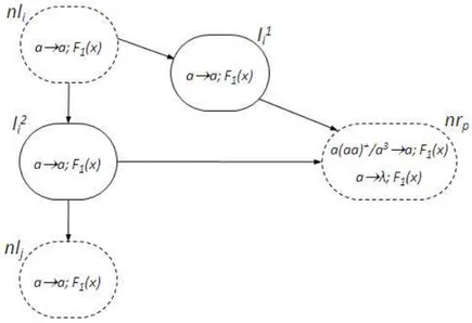
(i) A deterministic add instruction li : ADD(rp), lj, lj, for some p ∈ {2, . . . , m}
and i, j ∈ {0, 1, . . . , n} ∪ {h}, is simulated by the module presented in Figure 1.
1
Notice that, because of the way the firing of the rules has been defined, in general there is no upper bound on how many rules fire for each transition.
Figure 1: Module for the deterministic ADD instruction
(ii) A deterministic add instruction to register r1, li : ADD(r1), lj, lj, for
some i, j ∈ {0, 1, . . . , n} ∪ {h} is simulated by a module as the one shown in Figure 1, where neuron l1i is removed and neuron nr1 has no
rules.
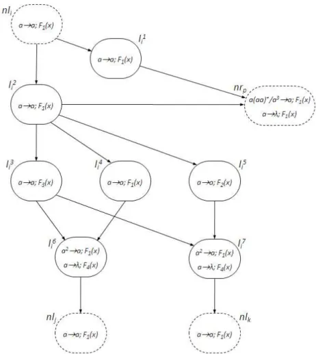
(iii) A non-deterministic add instruction, li : ADD(rp), lj, lk, for some p ∈
{2, . . . , m} and i, j, k ∈ {0, 1, . . . , n} ∪ {h} is simulated by the module shown in Figure 2; Again, as in the deterministic case, li : ADD(r1), lj, lk
(i.e., a non-deterministic add instruction to register 1) is simulated by a module as the one in Figure 2, but in which neuron l1i is removed and neuron nr1 has no rules inside.
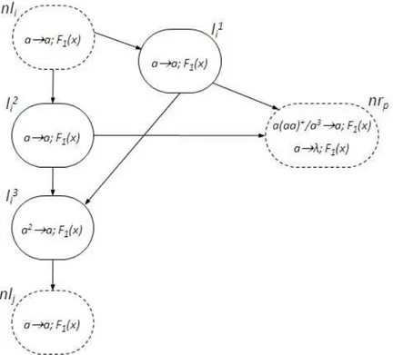
(iv) A sub instruction, li : SUB(rp), lv, lw, for some p ∈ {2, . . . , m} and
i, j, k ∈ {0, 1, . . . , n} ∪ {h} is simulated by the module shown in Figure 3.
Neuron nrj, for each j ∈ {1, · · · , m}, corresponds to the register rj
of M . Neuron nlj, for each j ∈ {0, 1, . . . , n} ∪ {h}, corresponds to the
(starting point of) instruction lj in the set I. In the initial configuration of
Π all neurons are empty, except the neuron nl0 corresponding to the initial
instruction of M that has 1 spike. The output neuron of Π is defined to be nr1 corresponding to register r1 of M (we recall that such register is only
subject to add instructions).
Finally, to complete the specification of the modules, we select the prob-ability distribution functions associated to the rules as follows:
Figure 2: Module for the non-deterministic ADD instruction
and variance σ2, which we shortly denote as N (µ, σ2), where we set µ1 = 1 and σ2 = 0 so that F1(x) = H(x − 1), where H(x) is the
Heaviside unitary step function2;
• F2(x) is defined to be N (µ2, σ2), with µ2 = 2;
• F3(x) is defined to be 0.5H(x − 1) + 0.5H(x − 2) , i.e., F3(x) is the
discrete uniform distribution in {1, 2});
• F4(x) is defined to be N (µ4, σ2), with µ4 = 0.5.
We now show how, because of the selected distributions of firing rules, each instruction of the register machine can be correctly simulated by the corresponding presented module.
2The Heaviside unitary step function H(x) is defined as H(x) = 0 if x < 0, H(x) = 1
Figure 3: Module for the SUB instruction
Let us suppose that, at an arbitrary time t, the register machine M is in a given configuration, in which it is to execute the instruction at label li
with a given state of r1, r2, . . . , rm registers, and suppose that the SSN P
system Π is in a configuration that corresponds to that of M , that means:
• neuron nri contains a number of spikes that is twice the contents of
register ri, for i = 2, 3, . . . , m;
• neuron nr1contains a number of spikes equal to the contents of register
r1;
• all other neurons are empty except neuron nli that contains exactly 1
Notice that, by construction, the initial configuration of Π corresponds to the initial one of M .
Consider now the various possible cases for the instruction li that M
starts executing at time t.
• li: ADD(rp), lj, lj (deterministic add) – module shown in Figure 1.
Suppose first that p 6= 1. Then, the execution of instruction li is
simulated in Π in the following way. At time t + 1 neuron nli fires
(with probability 1, because of the chosen distributions), one spike is introduced (at time t + 1, hence instantaneously) in neurons li1 and l2i. At time t+2 neurons li1and l2i fire with probability 1 and two spikes are added to neuron nrp. Also, at time t + 2, one spike is added to neuron
nlj. Except the ones mentioned, no other rule can fire in neurons l1i, li2
and nrp. Then, Π reaches, starting from the supposed configuration,
and with probability 1, a configuration that corresponds to the state of M after the execution of instruction li. If p = 1, the execution of
instruction li is simulated in a similar way, the only difference being
that only 1 spike is deposited in neuron nr1 at time t + 2. Thus, again
Π reaches with probability 1 a configuration that corresponds to the state of M after the execution of instruction li.
• li: ADD(rp), lj, lk (non-deterministic add) – module shown in Figure
2. In this case, the execution of the instruction li is simulated in Π as
follows. We only describe the case when p 6= 1, the non-deterministic add to register r1 is similar. At time t + 1, neuron nli fires with
probability 1, and at the same time one spike is introduced in neuron l1i and li2. At time t + 2, neurons li1 and l2i fire with probability 1, two spikes are then added to the neuron nrp and one spike is added to
neurons l3i, l4i and l5i. Neurons l4i and l5i fire, with probability 1, at time t + 3 and t + 4, respectively, emitting one spike to neuron l6i and l7i. In neuron l3
i, the rule a → a; F3(x) fires at a time that is either t + 3
or t + 4, with equal probability 2−1, and l3i emits one spike to neurons l6i and l7i: this probabilistic choice of the firing time in li3 simulates the non-deterministic choice of the ADD instruction.
In fact, if neuron l3
i fires at time t + 3, then one spike is sent to both
neurons li6 and l7i. The rule a2 → a; F1(x) fires with probability 1 in
neuron l6i at time t+4, sending one spike to neuron nlj. The forgetting
rule in neuron l7
i fires with probability 1 at time t + 3.5. At time t + 4,
the spike emitted by neuron l5i also reaches neuron l7i, the forgetting rule is enabled and it fires, with probability 1, at time t + 4.5.
If neuron l3i fires at time at time t + 4, the spike that was deposited in neuron l6
i by the firing of li4 at time t + 3 gets consumed, with
spike deposited at time t + 4 in l6i by the firing of neuron l3i enables again the forgetting rule of neuron l6i, and the spike present in l6i is consumed, with probability 1, at time t + 4.5. Also, at time t + 4, 2 spikes are deposited in neuron li7 (coming from neurons li5 and li3). This allows the rule a2→ a; F1(x) in neuron l7i to fire at time t+5 with
probability 1 and to send 1 spike in neuron nlk. In both considered
cases, when 1 spike reaches either neuron nlj or nlk, no rule can fire
anymore in neurons l1i, l2i, · · · , l7i and nrp.
The system Π can only execute, when starts from the supposed config-uration, with probability 1, the above described transitions. Therefore, Π reaches, with probability 1, the configuration that corresponds to the state of M after the instruction li has been executed.
• li : SU B(rp), lj, lk (non-deterministic sub) – module shown in Figure
3. The execution of instruction li is simulated in Π in the following
way. At time t + 1, neuron nli fires with probability 1 and one spike
is added to neuron nrp and one spike is added to both neurons l1i and
l2i. Neuron li1 fires at time t + 2 with probability 1 and deposits one spike in neuron l3
i. Also, neuron li2 fires, with probability 1, at time
t + 2 and deposits one spike in neuron l4i. Which rules fires in neuron nrp and at which time depends on the contents of the neuron at time
t. There are the two possible cases.
(i) The number of spikes in neuron nrp at time t is 0. Then, the
forgetting rule a → λ; F1(x) consumes the single spike present in
the neuron, at time t + 2, with probability 1.
(ii) The number of spikes in neuron nrp at time t is 2k with k >
0. Then, the rule a(aa)+ → a; F
1(x) fires at time t + 2 with
probability 1, depositing one spike in neuron l3i.
Notice that both rules present in neuron nrp consume an odd number
of spikes and then, once a rule is applied, no other rule in such neuron is enabled anymore.
In the case (i) only one spike reaches neuron l3i at time t + 2, and this spike is consumed, with probability 1, by using the forgetting rules, at time t + 3. Also, only one spike is deposited in neuron l5
i at time t + 3,
which fires, with probability 1, at time t + 4 depositing one spike in neuron nlk.
In the case (ii), two spikes are deposited in neuron li3 at time t + 2, which enable the rule a2 → a; F1(x). Neuron l3i then fires, with
probability 1, at time t + 3, depositing one spike in neuron nlj and one
spike in neuron l5i. Neuron li5 has two spikes at time t + 3 which are consumed, with probability 1, by the forgetting rule a2 → λ; F1(x) at
Starting from the supposed configuration Π can only execute, with probability 1, the above described transitions. Therefore, Π reaches, with probability 1, the configuration that corresponds to the state of M after the instruction li has been executed.
The execution of an instruction (ADD or SUB) in M followed by the HALT instruction is simulated in Π by simulating the corresponding in-struction (ADD or SUB) as described above and then sending 1 spike to the neuron nlh. By construction, neuron nlhdoes not have any outgoing synapse
to other neurons. Hence, the firing of its rule a → a; F1(x) consumes the
spike without sending any. Thus, also in this case Π halts in a configuration that correspond to the situation of M when the register machine halts.
From the above description, it is clear that Π can be composed using the presented modules in such a way that can simulate each computation of M and each computation in Π can be simulated in M . Therefore, the Theorem follows.
A remark concerns the dashed neurons shown in Figures 1,2, and 3. They represent the neurons shared among the modules. In particular, this is true for the neurons corresponding to the registers of M . Each neuron nrp, with p ∈ {2, 3, · · · , m} subject of a SUB instruction sends a spike to
several, possibly to all, neurons l3i, i = 0, 1, . . . , n, but only one of these also receives at same time a spike from the corresponding neuron li1. In all other cases, the other neurons forget the unique received spike.
A last comment closes the proof – it concerns the probabilities of the computations in Π. Each numbers x ∈ N (Π) is obtained with a proba-bility p(x) greater than zero. However not all the numbers in N (Π) are obtained in Π with the same probability. Indeed, for every computation c in M such that Out(c) = x, there is a probability 2−uc that Π simulates
exactly such computation where uc is the number of non-deterministic ADD
instructions executed in c. Therefore, the overall probability px is given by
P
c∈M |Out(c)=x2−uc.
2
5
Experiments on the Reliability of SSN P
Sys-tems
The SSN P system Π constructed in the proof of Theorem 4.1 works cor-rectly because of the appropriate choice of the probability distributions for the firing times associated to the rules in the neurons. In fact, the chosen distributions constrain the possible computations of Π in a way that the register machine M is able to simulate all the computations of Π and vice versa.
It was crucial in Theorem 4.1 that some of the chosen probability distri-butions had zero-variance. It is interesting to understand what happens to the correctness of the computation when this is not true anymore. In other words, what happens if we use the modules defined in Theorem 4.1 but we select, for all of them, a value of σ2 > 0? In informal words, this corresponds to increase the degree of non-synchronization in the constructed SSN P sys-tem: more variance is admitted for the distributions, more non-synchronous is the obtained system. As mentioned in the Introduction, in some cases asynchronous spiking neural P systems are not universal [4], so we conjec-ture that having distributions with non-zero variance makes more difficult (if not impossible) to simulate a register machine, with good “reliability”.
Therefore, from a computational point of view it is interesting to under-stand how the asynchrony present in the system, influences the ability for the system to correctly simulate a register machine. Moreover, considering dis-tributions with non-zero variance is interesting also from a biological point of view: spiking in neurons is the result of biochemical reactions, which are inherently random processes, hence they generally have a non-zero variance associated to their distributions.
As it has been shown in Theorem 4.1, by using σ2 = 0, each of the considered SSN P modules simulates the corresponding register machine instruction. When σ2 > 0 such an equivalence may not exists anymore, since the synchronization of the neurons in the modules is crucial. For example, consider the following transitions of the module corresponding to the deterministic ADD instruction, as shown in Figure 1. Neurons l1i and li2 simultaneously receive 1 spike, but it may happen that the rule in li1 neuron fires at time t and the one in neuron l2i fires at time t + δ, where δ depends on σ2 and may be large enough to make the two spikes in neuron nrp to
be consumed, one after the other, without actually increasing the number of spikes in neuron nrp as it should be done for a proper simulation of the
ADD instruction.
For an SSN P systems Π constructed as described in Theorem 4.1 we define the notion of correct simulation of a single instruction of the register machine M . We say that Π simulates correctly the instruction with label li
of M (suppose that li is followed by the instruction with label lj) when the
following thing is true. If Π starts from the configuration that corresponds to the configuration of M when instruction li is started, then Π executes a
sequence of transitions that leads to the configuration of Π that corresponds to that of M after the instruction li has been executed and, during these
transitions, the contents of all the neurons of Π, except nli and nlj, have
not been modified.
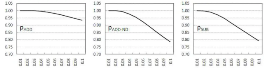
Let pADD, pADD−N D and pSU B be the probability that Π simulates
correctly the a deterministic ADD instruction, a non-deterministic ADD instruction and the SUB instruction of M , respectively. Theorem 4.1 shows
that, when σ2 = 0 is used, we have that pADD, pADD−N D and pSU B are
all equal to 1. When σ2 > 0, this is not true anymore. To quantitatively evaluate the effect of the variance σ2 we have developed a simulator of SSN P systems3.
We report the outcome of simulations conducted to evaluate probabilities pADD, pADD−N D and pSU B when varying the variance σ2 > 0. We present
in Figure 4 the obtained results for pADD, pADD−N D and pSU B when σ2 is
varied in the range [0.01, 0.1]. These probabilities have been computed with 10000 simulation batches for every value of σ2, with confidence level of 95%. The width of the confidence intervals for the simulation results is in each case below 0.1%, too narrow to be shown in Figure 4.
Figure 4: Probabilities pADD, pADD−N D and pSU B for values of σ2 in
[0.01, 0.1]
To give a quantitative feeling to the reader, we underline this well-known fact: the probability that a random sample of a random variable distributed as N (µ, σ2) is far from µ more than σ is about 0.3, more than 2σ is about 0.05 and more than 3σ is about 0.003. For instance, when σ2 = 0.1, a random sample drawn from distribution F1(x) will have probability 0.3 of
being outside interval [0.7, 1.3] and probability 0.05 of being outside interval [0.4, 1.6]. Such variability brings asynchrony in the considered instruction modules and this makes possible many transitions, which would not occur if σ2 = 0. Therefore, it is not surprising that probabilities pADD, pADD−N D
and pSU B decrease as σ2 increases (as Figure 4 shows).
From Figure 4 it is also possible to observe that probabilities pADD,
pADD−N D and pSU B are close to 1 (i.e., the corresponding instructions are
simulated correctly) when σ2 takes values in the lower part of the considered range of variation. This result supports the idea that Π is able to simulate correctly, with high probability, long computations of the register machine M even for values of σ2 > 0.
To understand more precisely how Π can simulate M in a reliable way, when a non-negative variance σ2is considered, we define a probability metric called the reliability of Π, which we use to characterize the ability of Π to compute correctly a number in Out(M ).
The reliability of a system is defined as a function R(t), t ≥ 0, which expresses the probability that in the interval of time [0, t] the system has been working correctly, supposing that the system was working correctly at time t = 0 (this follows the standard definition of reliability. See, e.g., [11]). The definition of the correct behavior of the system has to be given with reference to a specification of the system, or alternatively can be given with respect to another system, which is assumed to be always correct. We choose the second approach: In what follows, we shall evaluate the reliability of the SSN P system Π (when varying σ2) by comparing the sequences of transitions performed by Π against the ones that are performed by a register machine M .
Precisely, we define the reliability RMΠ(n) as the probability that Π sim-ulates correctly a sequence of n instructions executed by M , when M starts from the initial configuration and Π starts from the corresponding one.
In what follows we experiment on a particular SSN P system (and on a particular computed set of numbers) how the variance of firing rules dis-tribution times systems affects the reliability. For this purpose we consider, the set of natural numbers P ow2 = {n | n = 2m, m ≥ 0} that is the set of natural numbers that are power of 2 (actually, P ow2 is also a non-semilinear set of natural numbers).
The set P ow2 can be computed, for instance, by the following register machine M0 = (2, {l0, l1, . . . , l8, lh}, l0, lh, I). The idea is that M0 moves
the contents of register 1 to 2 and back, and, in this case, doubles the contents; ADD with label l1is a “dummy” instruction, used only for the
non-deterministic choice between continuation of the computation or halting: the object added is, in fact, subtracted again in the SUB, at l2 or l8.
Instructions I are the following ones.
l0: ADD(r1), l1, l1 l1: ADD(r1), l8, l2 l2: SU B(r1), l3, l3 l3: SU B(r1), l4, l5 l4: ADD(r2), l3, l3 l5: SU B(r2), l6, l1 l6: ADD(r1), l7, l7 l7: ADD(r1), l5, l5 l8: SU B(r1), lh, lh lh: HALT
Let Π be the SSN P system that corresponds to M , built as described in Theorem 4.1, using the modules presented in Figures 1, 2 and 3 and having σ2> 0.
We evaluate the function RMΠ0(n) by using simulations for values of σ2 close to 0.01. We show in Figure 5 the simulation results, which were com-puted with 100000 batches of simulation for each considered value of σ2, with a confidence level of 95%. The width of confidence intervals is within 5% of the estimated values (they are not shown in Figure 5 for the sake of clarity).
Figure 5: Reliability function RMΠ0(n) for different values of σ2 The reliability functions plotted in Figure 5 show that, as σ2 increases, Π has higher and higher probability of performing incorrect simulations. However, for σ2 = 0.01, the probability that Π is able to simulate correctly computations of M0 composed by 15.000 instructions is still quite high, 0.9. For such value of σ2, the value of the reliability function at n = 1000 is of about 0.996. This means that, if we restrict our attention to the computations of M0 that are composed by less than 1000 instructions and consider σ2 = 0.01, then we observe that Π can simulate correctly these computations with probability 0.996.
We can also use the above described procedure do design systems with arbitrary reliability.
In fact, constructing an opportune Figure 5, one can identify, for an arbitrary register machine M , the maximal value of σ2 for which is possible
to construct, using the approach given in Theorem 4.1, an SSN P system Π with a reliability RMΠ(n) that is at least k, with k an arbitrarily chosen constant 0 ≤ k ≤ 1.
Finally, it is important to mention that, for a given register machine M , several equivalent SSN P systems can be constructed, using different constructions (Theorem 4.1 shows only one of them). These SSN P systems, even equivalent from a computational point of view, can have very different reliability. A way to get different SSN P systems, with different reliability, is, for instance, to construct different modules to simulate the register machine instructions.
For instance, consider the module shown in Figure 6, for which we define F1(x) = N (1, σ2). It is easy to check that, when σ2 = 0, the module shown
in Figure 6 (we call it ADD2) is equivalent to the module shown in Figure 1 (we call it ADD). In fact, both of them, for σ2 = 0, simulate correctly the (deterministic) ADD instruction of the register machine.
However, having an intermediate neuron, makes the module in Figure 6 more reliable than the module in Figure 1. We can check that by calcu-lating, using the above described procedure, pADD2. This is clear from the
comparison between pADD and pADD2 presented in Figure 7.
Figure 7: Probabilities pADD1 and pADD2 for values of σ2 in [0.01, 0.1]
6
Perspectives
Constructing reliable and powerful computational devices by combining sev-eral simple (bio-inpired) units has been studied intensively in computer sci-ence, starting from classical cellular automata. Recently, several researchers are investigating the possibility of constructing fault-tolerant systems, es-pecially computer architectures and software by using ideas coming from nanotechnology and from biological processes (see, e.g., [12]).
In our case, we have investigated, in the framework of SN P systems, a kind of fault-tolerance that concerns the possibility to obtain powerful (universal) computing devices, when using computational units that are simple and non-synchronized. We have defined a stochastic version of SN P systems (SSN P system) where to each rule is associated a stochastic “waiting” time and we have presented a preliminary study that shows how the degree of asynchrony (expressed as variance) among the neurons can influence the ability of an SSN P systems to simulate/executed in a reliable way the program of a register machine.
The topic is very general and several lines of research can be followed. The most interesting one concerns the possibility to implement powerful computing devices (possibly, universal) using SSN P systems having an high degree of asynchrony, i.e., with distributions associated to the firing times with an high variance. When is this possible? What is the price to pay for that? An important question that we have not answered in the paper is the following one. Can the topology of the network influence the reliability of the constructed system? (in this case one may find motivations and
inspira-tions from the topology of the real networks of neurons). Another relevant question: Can the redundancy (i.e., number of neurons and connections) help in obtaining more reliable systems? This appears to be true, at least in view of the better reliability (Figure 7) of the module presented in Figure 6 compared to that of the module shown in Figure 1. How much redundancy can help and what is the best way to use redundancy ?
Another line of research concerns the study of class of SSN P system where reliability can be analytically investigated. For instance, in case of exponential distributions, one should be able to construct an equivalent Markov chain and then studying in an analytical manner the reliability of the system. Are there other cases where this is possible? In general, as seen in Section 5, there is a link between the type of transitions executed and the reliability of the system (not all transitions are equally relevant/dangerous for the reliability of an SSN P system). Is there a possibility to limit the number of certain type of transitions? (this is, of course, very much linked to the number of minimal instructions of a certain type that one has to use in a register machine program - hence one may find links between reliability and Kolmogorov complexity, [29]).
References
[1] A. Carbone and N. Pierce, eds. DNA Computing, 11th International Workshop on DNA Computing. LNCS 3892, Springer, 2005.
[2] M. Cavaliere and V. Deufemia, Further results on time-free P systems. Intern. J. Found. Computer Sci., 17(1), 2006.
[3] M. Cavaliere, O. Egecioglu, O.H. Ibarra, S. Woodworth, M. Ionescu, and Gh. P˘aun, Asynchronous spiking neural P systems, Tech. Report 9/2007 Microsoft Research - University of Trento, Centre for Compu-tational and Systems Biology. Available at www.cosbi.eu.
[4] M. Cavaliere, O. Egecioglu, O.H. Ibarra, M. Ionescu, Gh. P˘aun, and S. Woodworth, Asynchronous Spiking Neural P Systems; Decidability and Undecidability. Proceedings 13th International Meeting on DNA Computing, DNA13, Lecture Notes in Computer Science, LNCS 4848, Springer, 2007.
[5] M. Cavaliere and D. Sburlan, Time-independent P systems. In Mem-brane Computing. International Workshop WMC5, Milano, Italy, 2004, LNCS 3365, Springer, 2005, pp. 239–258.
[6] M. Cavaliere and C. Zandron, Time-Driven Computations in Membrane Systems. In [8].
[7] G. Clark, T. Courtney, D. Daly, D. Deavours, S. Derisavi, J. M. Doyle, W. H. Sanders, P. and Webster, The M¨obius Modeling Tool. Proceed-ings International Workshop on Petri Nets and Performance Models (PNPM’01), IEEE Computer Society, 2001.
[8] M. A. Guti´errez-Naranjo et al., eds., Proceedings of Fourth Brainstorm-ing Week on Membrane ComputBrainstorm-ing, Febr. 2006, Fenix Editora, Sevilla, 2006.
[9] W. Gerstner, Population Dynamics of Spiking Neurons: Fast Tran-sients, Asynchronous States, and Locking. Neural Computation, 12, 43, 2000.
[10] W. Gerstner, and W. Kistler, Spiking Neuron Models. Single Neurons, Populations, Plasticity. Cambridge Univ. Press, 2002.
[11] J. C. Laprie, Dependability - Its Attributes, Impairments and Means. In [26].
[12] J.R. Heath, P.J. Kuekes, G.S. Snider, S. Williams, A Defect-Tolerant Computer Architecture: Opportunities for Nanotechnology. Science, 280, 1998.
[13] O.H. Ibarra, A. P˘aun, Gh. P˘aun, A. Rodr´ıguez-Pat´on, P. Sosik, and S. Woodworth: Normal forms for spiking neural P systems. Theoretical Computer Scienc, 372, 2-3, 2007.
[14] M. Ionescu, Gh. P˘aun, and T. Yokomori, Spiking neural P systems. Fundamenta Informaticae, 71(2-3), 2006.
[15] W. Maass, On the Computational Power of Noisy Spiking Neurons. Advances in Neural Information Processing Systems, 8, 1996.
[16] M. Madhu, Probabilistic Rewriting P Systems. Intern. J. of Found. of Computer Sci.. 14 (1) 2003.
[17] M. A. Marsan, Stochastic Petri Nets: An Elementary Introduction. In: Advances in Petri Nets, LNCS 424, Springer, Berlin, 1989.
[18] M. Minsky, Computation – Finite and Infinite Machines. Prentice Hall, Englewood Cliffs, NJ, 1967.
[19] M. Muskulus, D. Besozzi, R. Brijder, P. Cazzaniga, S. Houweling, D. Pescini, and G. Rozenberg, Cycles and Communicating Classes in Mem-brane Systems and Molecular Dynamics. Theoretical Computer Science, 372, 2-3, 2007.
[20] Gh. P˘aun, Spiking Neural P Systems: A Tutorial. Bulletin of the EATCS, 91 (Feb 2007).
[21] Gh. P˘aun, Membrane Computing – An Introduction. Springer, Berlin, 2002.
[22] Gh. P˘aun, M.J. P´erez-Jim´enez, and G. Rozenberg, Spike trains in spik-ing neural P systems. Intern. J. Found. Computer Sci., 17(4), 2006.
[23] D. Pescini, D. Besozzi, G. Mauri, and C. Zandron, Analysis and Simu-lation of Dynamics in Probabilistic P Systems. In [1].
[24] A. Obtulowicz and Gh. P˘aun, (In Search of) Probabilistic P Systems. BioSystems 70, 2003.
[25] G. Rozenberg and A. Salomaa, eds., Handbook of Formal Languages, 3 Volumes. Springer-Verlag, 1997.
[26] B. Randell, J. C. Laprie, H. Kopetz and B. Littlewood eds., Predictably Dependable Computing Systems, Springer-Verlag, 1995.
[27] A. Salomaa, Formal Languages. Academic Press, 1987.
[28] K. H. Trivedi, Probability and Statistics with Reliability, Queuing, and Computer Science Applications. John Wiley and Sons, New York, 2001.
[29] M. Li, P. Vit´any, An Introduction to Kolmogorov Complexity and Its Applications. Springer, 1997.


![Figure 7: Probabilities p ADD1 and p ADD2 for values of σ 2 in [0.01, 0.1]](https://thumb-eu.123doks.com/thumbv2/123dokorg/2948018.23197/20.892.215.677.194.494/figure-probabilities-p-add-p-add-values-s.webp)
