Derivative Riemann problem and ADER schemes

(1)

Dottorato di Richerca in Matematica

XVII ciclo

VLADIMIR A. TITAREV

Derivative Riemann problem

and ADER schemes

Ph.D. thesis

SUPERVISOR: PROFESSOR E.F. TORO OBE

(2)

Acknowledgments

I would like to thank the Department of Mathematics, University of Trento, Italy, for giving me a possibility to study and do research as well as travel to numerous conferences. Many thanks are to my supervisor, Professor E.F. Toro OBE, for his guidance, support and encouragement during the course of this research.

Finally, I thank my parents for their continuous support during this exceedingly long project.

(3)

Introduction

Hyperbolic conservation laws arise in areas as diverse as shallow water flows, compressible gasdynamics, turbulence modelling, turbomachinery, plasma modelling, rarefied gas dynamics and many others. Analytical solutions are available only in very few special cases and numerical methods must be used in practical applications. The present thesis is devoted to the construction of numerical schemes of very high-order of accuracy for solving nonlinear hyperbolic conservation law. In designing such schemes one faces at least three major difficulties. One of them concerns the preservation of high accuracy in both space and time for multidimensional problems containing source terms. Another one concerns conservation; this is mandatory in the presence of shock waves. The other very important issue relates to the generation of spurious oscillations in the vicinity of strong gradients; according to Godunov’s theorem [18] these are unavoidable by linear schemes of accuracy greater than one. These oscillations pollute the numerical solution and are thus highly undesirable. To avoid generating spurious oscillations, non-linear solution-adaptive schemes must be constructed.

Each one of these difficulties is in itself not easy to resolve; the simultaneous resolution of all three difficulties above represents a formidable task in the numerical analysis of hyperbolic conservation laws.

At present, there are various approaches for constructing numerical schemes that attempt to overcome the above difficulties. The class of Godunov-type methods for solving numerically hyperbolic conservation laws is often regarded as one of the most successful. The original first-order scheme of Godunov [18] uses the self-similar solution of the local Riemann problem with piece-wise constant initial data to compute the upwind numerical flux. The extension to second order of accuracy in time and space can be carried out, amongst other ways, by using a non-oscillatory piece-wise linear reconstruction of data from cell averages. It appears as if it was Kolgan [25] who first proposed to suppress spurious oscillations by applying the so-called principle of minimal values of derivatives, producing in this manner a non-oscillatory (TVD) Godunov-type scheme of second order spatial accuracy. Further, more well-known, developments are due to van Leer [82]. In multiple space dimensions unsplit second-order non-oscillatory methods were constructed by Kolgan [27, 26], Tiliaeva [48], Colella [12] and many others.

TVD methods avoid oscillations by locally reverting to first order of accuracy near discontinuities and extrema. They are therefore unsuitable for applications

(5)

involving long time evolution of complex structures, e.g. in acoustic and compressible turbulence. In these applications extrema are clipped as time evolves and numerical diffusion may become dominant. Uniformly very high order methods, both in time and space, are needed for such applications.

Essentially non-oscillatory schemes [19] can be regarded as uniformly high order extensions of Kolgan- van Leer approach in which the data in each cell is represented by polynomials of arbitrary order rather than linear ones. The numerical solutions obtained by these methods are, at least to the eye, free from spurious oscillations.

The key idea in the rth _{- order ENO reconstruction procedure used in [19, 43, 7] is}

to consider r possible stencils covering the given cell (in one space dimension) and to select only one, the smoothest, stencil. The reconstruction polynomial is then built using this selected stencil. The WENO reconstruction [30, 22] takes a convex combination of all r stencils with non-linear solution-adaptive weights. The design of the weights involves local estimates of the smoothness of the solution in each possible

stencil so that the reconstruction achieves (2r − 1)th _{- order of spatial accuracy in}

smooth regions and emulates the rth_{- order ENO reconstruction near discontinuities.}

A more refined version of the one-dimensional WENO reconstruction is the so-called monotonicity-preserving WENO (MPWENO) [3] which is a combination of

increasingly high order (e.g. 9th _{order) WENO and a monotonicity preserving (MP)}

constraint [46].

Essentially non-oscillatory schemes can be divided into finite-difference schemes and finite-volume schemes. Finite-difference schemes, pioneered in [43] and further developed in [22, 3] seem to be more popular for academic applications due to their simplicity and low cost, e.g. [44], but are restricted to smooth structured meshes. Finite-volume schemes are more expensive and complicated, but can be used on arbitrary non-smooth or/and non-structured meshes and are therefore of more interest to us. In multiple space dimensions these schemes have been developed in [7, 1, 33, 21, 41, 52]. A comparison of finite-difference and finite-volume ENO schemes can be found in [8].

Another very interesting class of very-high order methods for hyperbolic systems is the class of Discontinuous Galerkin (RKDG) Finite Element Methods, which consists of Runge-Kutta DG methods [9, 2, 10, 11] and Space-Time DG methods [79, 80, 81]. These schemes combine the finite-element idea of representing the data locally inside each cells by means of spatial polynomials and using the Riemann problem solution in the computation of the intercell flux. In fact, the first-order DG scheme boils down to the original Godunov method [18]. The key advantage of DG methods over finite-volume schemes lies in their locality: since the data

(6)

representation in each cell is stored and evolved by the method no reconstruction procedure is required. This is especially important when using unstructured meshes, e.g. triangles in two space dimensions. Locality of the method also greatly helps in implementing h-refinement algorithms. However, a pending problem in the RKDG methods is the construction of some sort of the limiting procedure to suppress the spurious oscillations. The present approaches, such as the TVD limiter or the use of Hermite WENO schemes [36, 35], do not seem to completely resolve the issue.

We should also mention the class of Compact Difference Methods of Tolstykh and co-workers [55, 56, 57, 59, 60, 58]. These schemes achieve arbitrary order of

spatial accuracy, e.g. in last two references up to 57th _{order is reported. However,}

the compact approximations are, in general, not monotone and some sort of a limiter must be used to avoid spurious oscillations. The application of the limiter is helped by the fact, that the oscillations are typically contained in 2-3 cells around the discontinuity only.

All the schemes discussed above meet the requirement of very high-order spatial accuracy. Matching time accuracy to space accuracy, however, remains an issue in all of the above approaches due to the use Runge-Kutta methods for time evolution. To avoid spurious oscillations these Runge-Kutta methods must be TVD [42]. This leads to accuracy barriers: the accuracy of such methods cannot be higher than fifth [42]. Moreover, fourth and fifth order methods are quite complicated and have reduced stability range. In most practical implementations reported, when the solution is not smooth, a third order TVD Runge-Kutta method has been used, e.g. [3].

Although increased order of spatial discretisation improves accuracy for some problems such schemes converge with third order only when the mesh is refined and thus should be regarded as third order schemes. For some applications, such as numerical simulation of compressible turbulence and wave propagation problems involving long-time evolution it may be beneficial to use schemes which converge with higher order both in time and space.

A recent approach for constructing schemes of very high order of accuracy is the ADER (Advection-Diffusion-Reaction) approach [71, 72], which stems from the modified Generalised Riemann Problem (MGRP) scheme [64], which in turn is a simplification of the GRP-type schemes [4, 31]. ADER allows the construction of arbitrarily high-order accurate schemes, both in time and space. The original ADER idea was applicable to linear advection with constant coefficients only. In [71, 72] formulations were given for one, two and three-dimensional linear schemes

(7)

and time for both the one-dimensional and the two-dimensional case were reported. In [40, 39, 17] linear schemes for linear systems with constant coefficients of up to

6th _{order in space and time were constructed. These were then applied to acoustic}

problems and detailed comparison with other schemes was carried out.

The extension of the ADER approach to non-linear problems relies on the solution of the Derivative Riemann problem. The solution procedure for the DRP reported in [74] provides an approximation to the state variable along the t-axis in the form of a Taylor time expansion and relies, among other things, on the availability of an approximate-state Riemann solver for the non-linear conventional (piece-wise constant initial data) Riemann problem system. Construction of ADER schemes for the one-dimensional Euler equations using this Riemann problem solution has been reported in [49]. For the construction of schemes as applied to non-linear scalar equations in one space dimension see also [47]. Extension of ADER to scalar advection-diffusion-reaction equations in one space dimension is reported in [50],

where explicit non-linear schemes of up to 6th _{order are presented.}

This thesis is devoted to the further construction and generalization of the ADER advection schemes to the case of non-linear multi-dimensional conservation laws with reactive-like source terms. The main objective is three-fold. Firstly, we would like to extend the schemes to systems for which the solution of the conventional Riemann problem is not available or exceedingly complicated. To achieve this, we need to modify the Derivative Riemann problem solver. Secondly, we would like to extend the schemes to multidimensional non-linear hyperbolic systems with reactive-like source terms. Finally, we carry out truncation error and stability analysis of the schemes for the model linear advection equation with constant coefficients in one, two and three space dimensions.

The rest of the thesis is organized as follows.

In Chapter 1 we present the approximate solution of the Derivative Riemann problem. Conventionally, the Riemann problem for a system of conservation laws is defined as the Cauchy problem with initial conditions consisting of two constant states separated by a discontinuity at the origin [18]. A generalization of this is the so-called Generalized Riemann problem [4, 32], whereby a piece-wise linear data Riemann problem is posed and solved. A further generalization is to consider the Riemann problem for a system of equations with source terms and arbitrary piece-wise smooth initial data [29, 6, 74]. In particular, the initial conditions may consist of polynomials of arbitrary degree. Here we call such Riemann problem, the Derivative Riemann Problem, or DRP for short. The approximate solver described here provides an approximation to the state variable along the t-axis in the form

(8)

of a Taylor time expansion. To build up this expansion, the original DRP is reduced to a sequence of conventional Riemann problems for homogeneous advection equations. The leading term of the expansion is computed as the Godunov state of the conventional nonlinear Riemann problem, whereas the evaluation of higher-order terms involves the solution of linearized Riemann problems for spatial derivatives. Therefore, availability of an approximate-state Riemann solver for the non-linear conventional Riemann problem system is crucial for building up the approximate solution to the DRP.

Although exact or approximate-state Riemann solvers are available for a large variety of hyperbolic systems of conservation laws [65, 28], for complex nonlinear systems they may become very complicated or simply unavailable. It is therefore desirable to have a simple procedure for calculating the leading term of the state expansion which would not necessarily require a detailed knowledge of the Riemann problem solution. We develop a new modification of the DRP solver which differs from the original one in the way how the leading term of the Taylor time expansion is computed. That is, the new procedure does not require a Riemann solver for the nonlinear system to be solved. This method proceeds first to a non-linear evolution of the initial condition of a conventional Riemann problem, followed by a simple linearization of the Riemann problem, which leads to closed-form solutions. We illustrate the method by solving the DRP for the inviscid Burgers’ equation with a source term. The presented results demonstrate that both the original and modified solvers can maintain a really arbitrary order of accuracy even when the solution to the problem contains a shock wave.

In Chapter 2 we present the general construction of the ADER schemes as applied to the non-homogeneous conservation laws in multiple space dimensions on Cartesian meshes. The ADER schemes have a standard one-step finite-volume form with intercell numerical fluxes obtained by performing time-space integration of the physical fluxes over cell faces. The computation of the ADER intercell flux essentially consists of three major steps. Firstly, since the scheme advances cell averages of the solution but the flux need point-wise values, a high-order polynomial reconstruction is carried out for each cell. In order to circumvent Godunov’s theorem [18] and avoid spurious oscillations the weighted essentially non-oscillatory procedure is used. We discuss the finite-volume WENO reconstruction in multiple space dimensions and present extensions of [7, 22, 41] to higher orders and three spatial dimension [52]. Next, at each cell interface (or spatial quadrature point for spatial integration over the side/face in multiple space dimensions) we have the Derivative Riemann problem with the initial data in the form of reconstruction polynomials.

(9)

Using the DRP solver described in Chapter 1 we build up an approximate state and use it to obtain the numerical flux. The computation of the numerical source terms is then performed in a rather direct manner and involves application of the multidimensional quadrature.

The chapter is composed as follows: firstly, we describe the reconstruction procedure. Next, the scheme in one spatial dimension is presented. A special version, called ADER-TVD, is developed by replacing the first-order Godunov flux by the second-order TVD flux for each term of the ADER flux expansion leading to a much more accurate scheme. Finally, extension to the multiple space dimensions is carried out, which includes a special adaptation of the DRP solver from Chapter 1.

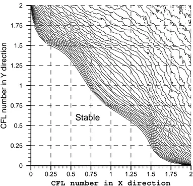
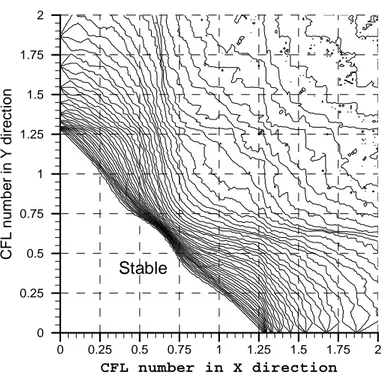
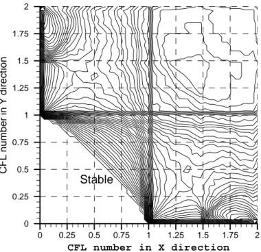
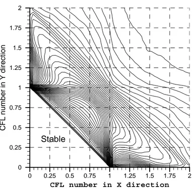
In Chapter 3 we carry out the stability and truncation error analysis of the schemes as applied to the model linear advection equation with constant coefficients in one, two and three space dimensions. We consider the schemes of different order of accuracy as well as different reconstruction stencils, e.g. upwind or downwind biased. The results of the analysis demonstrate analytically that the schemes do maintain the desired order of accuracy both in time and space and are stable under the normal Courant number. The stability region of the scheme is the same as that of the unsplit first-order Godunov method and the state-of-the-art ENO/WENO schemes.

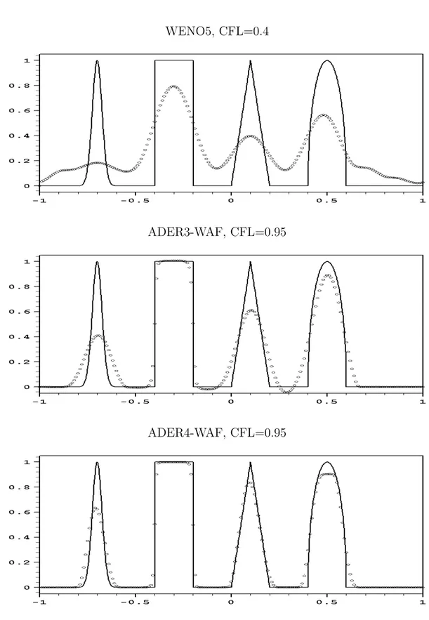
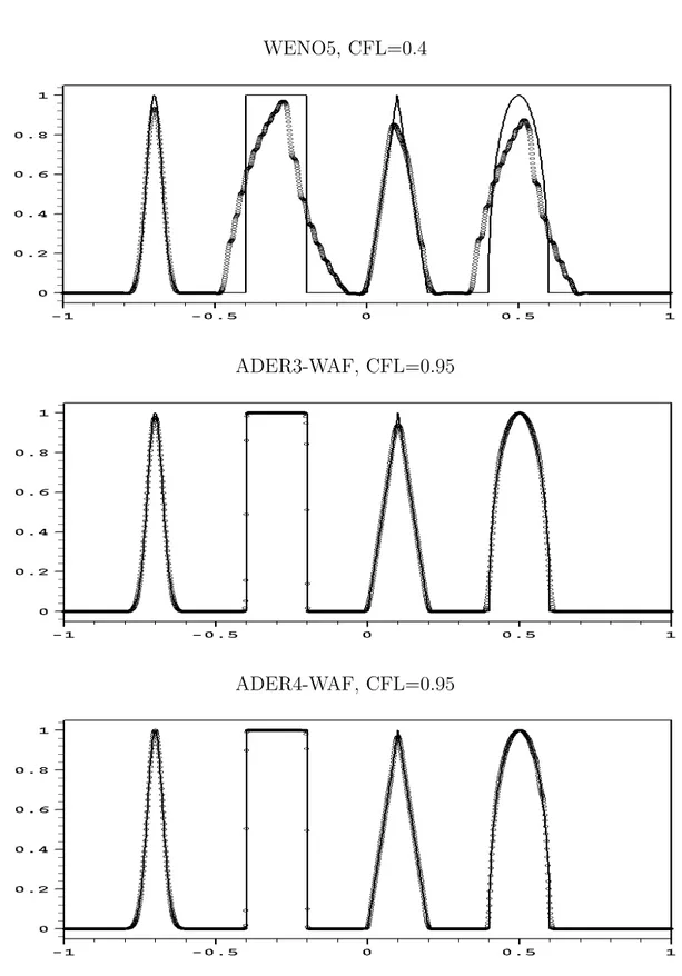
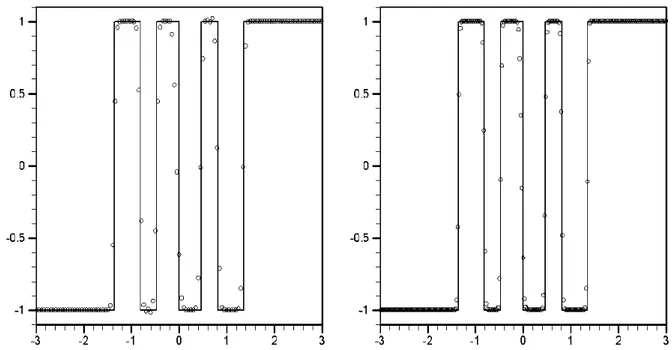
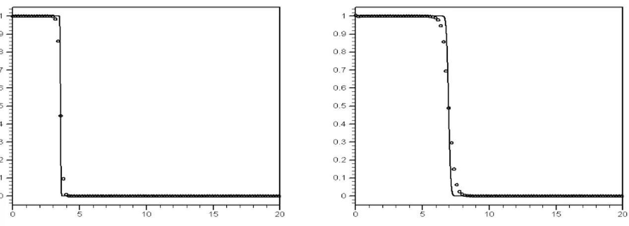
Numerical results are presented in Chapter 4 and are divided in three groups: scalar equations, nonlinear compressible Euler equations and nonlinear shallow water equations with source terms. In most of the cases we compare our schemes with the state-of-the art finite-volume WENO schemes [41] The convergence studies for a number of well-established test problems demonstrate the schemes compare well with the other modern methods, can maintain the desired very high order of accuracy in both time and space for nonlinear systems, and at the same time can be used for computing solutions with strong moving and possibly colliding discontinuities.

Our presentation is concentrated on the development of main ideas of the ADER flux and source term computation and is thus restricted to Cartesian meshes only. Recently, the approach has been extended to unstructured triangular meshes [23, 24]. All the basic technologies for the computation of the ADER flux, e.g. the solution of the Derivative Riemann Problem, remain the same except the reconstruction, which is now carried out on triangles. In [24] non-oscillatory schemes of up to fourth order of temporal accuracy have been reported and applied to a number of test problems. Another very recent and promising direction of research on advection schemes are the so-called ADER-DG methods [14, 16, 15]. The basic idea of these methods

(10)

is to replace the Runge-Kutta time marching in the DG methods by the ADER-type temporal discretization. The resulting ADER-DG methods are one-step and of really arbitrary order of accuracy. The numerical results of the schemes of up to

6th _{order as applied to two-dimensional non-linear systems have been reported.}

The main results of the present thesis have been published in the following papers:

1. V.A. Titarev and E.F. Toro. Finite-volume WENO schemes for three-dimen-sional conservation laws. J. Comput. Phys., 201(1):238–260, 2004.

2. E.F. Toro and V.A. Titarev. ADER schemes for scalar non-linear hyperbolic conservation laws with source terms in three-space dimensions. J. Comput. Phys., 202(1):196–215, 2005.

3. V.A. Titarev and E.F. Toro. ADER schemes for three-dimensional nonlinear hyperbolic systems. J. Comput. Phys., 204(2):715–736, 2005.

4. V.A. Titarev and E.F. Toro. MUSTA schemes for multi-dimensional hyperbolic

systems: analysis and improvements. International Journal for Numerical

Methods in Fluids, 49(2):117–147, 2005.

5. E.F Toro and V.A. Titarev. TVD fluxes for the high-order ADER schemes. J. Sci. Comput., 24(3):285-309. 2005.

6. E.F. Toro and V.A. Titarev. Derivative Riemann solvers for systems of conservation laws and ADER methods. J. Comput. Phys., 212(1):150-165. 2006.

and in [51]. One more paper is to appear in J. Comput. Phys.:

E.F. Toro and V.A. Titarev. MUSTA schemes for systems of conservation laws. Main results have also been presented at a number of international conferences, including the 6th International Conference on Spectral and High-Order Methods, June 21-25, 2004, Brown University, RI, USA and The Tenth International Conference ”Hyperbolic Problems: Theory, Numerics and Applications”, September 13-17, 2004, Osaka, Japan.

(11)

1. Derivative Riemann Solvers

Introduction

Conventionally, the Riemann problem for a system of conservation laws is defined as the Cauchy problem with initial conditions consisting of two constant states separated by a discontinuity at the origin. A generalization of the conventional Riemann problem in which the piece-wise linear polynomials are used as the initial data has become to be known as the Generalized Riemann problem [4, 29, 6, 31, 32]. A further generalization is to consider the Riemann problem for a system of equations with source terms and arbitrary piece-wise smooth initial data [29, 6, 74]. In particular, the initial conditions may consist of polynomials of arbitrary degree. Here we call such Riemann problem, the Derivative Riemann Problem, or DRP for short.

This chapter is devoted to the construction of the approximate solution for the Derivative Riemann problem [74, 78]. Later we intend to use this solution in the design of the numerical schemes. We note that for the Godunov-type methods one does need the Riemann problem solution in the whole t − x space, but rather only along the t axis. Moreover, the complete solution is most probably impossible to construct for a sufficiently complex system. For example, a second-order accurate solution to the GRP problem for a rather simple system of the one-dimensional compressible Euler equations is already quite complicated [32] and probably is not practical.

The solution procedure reported here provides an approximation to the state variable along the t-axis in the form of a Taylor time expansion. To build up this expansion, the original DRP is reduced to a sequence of conventional Riemann problems for homogeneous advection equations. The leading term of the expansion is computed as the Godunov state of the conventional nonlinear Riemann problem, whereas the evaluation of higher-order terms involves the solution of linearized Riemann problems for spatial derivatives. Therefore, availability of an approximate-state Riemann solver for the non-linear conventional Riemann problem system is crucial for building up the approximate solution to the DRP.

Although approximate-state Riemann solvers exist now for a large variety of hyperbolic systems of conservation laws [65, 28], for complex nonlinear systems they may become very complicated or simply unavailable. It is therefore desirable to have a simple procedure for calculating the leading term of the state expansion

(12)

which would not necessarily require a detailed knowledge of the Riemann problem solution. Here we employ a recent EVILIN solver [69] to circumvent the problem of computing the leading term. The method proceeds first to a non-linear evolution of the initial condition of a conventional Riemann problem, followed by a simple linearization of the Riemann problem, which leads to closed-form solutions.

Finally, we illustrate the performance of the DRP solver with both methods for computing the leading term by solving the DRP for the inviscid Burgers’ equation with a source term. We first obtain an accurate numerical solution of the problem. Next, we use this solution to verify the accuracy and convergence rate of the approximate DRP solver, developed in this chapter.

1.1. Derivative Riemann problem and solution methodology The Derivative Riemann Problem or DRP for a hyperbolic system is the initial-value problem ∂tQ + ∂xF(Q) = S(x, t, Q) , Q(x, 0) = ( QL(x) if x < 0 , QR(x) if x > 0 .        (1.1)

where the initial states QL(x), QR(x) are two vectors, the components of which

are smooth functions of distance x. We introduce the notation DRPK to mean

the Derivative Riemann Problem in which K represents the number of non-trivial

spatial derivatives of the initial condition, K = max{KL, KR}, where KL and KR

are such that ∂(k)

x QL(x) ≡ 0 ∀k > KL , ∀x < 0 and ∂x(k)QR(x) ≡ 0 ∀k > KR , ∀x > 0 .

DRP0 means that all first (k = 1) and higher-order spatial derivatives of the initial

condition for the DRP away from the origin vanish identically; this case corresponds to the conventional piece-wise constant data Riemann problem.

The two initial states QL(x) and QR(x) are assumed to be smooth functions, for

example K−th order polynomials, defined respectively for x < 0 and for x > 0, with a discontinuity at x = 0. Away from x = 0 we could use the Cauchy-Kowalewski method to construct a solution Q(x, t) to (1.1), provided that all the smoothness assumptions of the Cauchy-Kowalewski theorem were met. Here we are interested

in the solution of DRPK, right at x = 0, where in fact the initial data may be

(13)

q q q q q q q q q (3) (2) (K) (1) (2) (3) (K) q(1) L L L L R R R R R L(x) (x) (0) (0) (0) (0) (0) (0) (0) (0) x=0 x q(x,0)

Figure 1.1. Information available in the DRPK for a scalar problem.

Figure 1.1 illustrates the initial conditions of the DRPK and the information

available at t = 0 at the origin x = 0. The initial data is, in general, discontinuous at x = 0. Away from x = 0 the initial data is smooth, with all spatial derivatives well defined and readily computed. At x = 0 we can define one-sided spatial derivatives, so that at the interface x = 0 we have jumps in spatial derivatives. These jumps will form the initial data for new (conventional) Riemann problems, as we shall explain below.

We seek a power series solution at x = 0 as a function QLR(t) of time t only.

Formally, we write the sought solution as

QLR(τ ) = Q(0, 0+) + K X k=1 h ∂_t(k)Q(0, 0+)i τ k k! , (1.2) where 0+ ≡ lim t→0+

t. The solution contains a leading term Q(0, 0+) and higher-order

terms with coefficients determined by ∂_t(k)Q(0, 0+). In what follows we describe a

method to compute each of the terms of the series expansion.

1.2. The leading term

The leading term Q(0, 0+) in the expansion accounts for the first-instant interaction

of the initial data via the governing PDEs, which is realized solely by the boundary

(14)

is found from the similarity solution of the following DRP0 ∂tQ + ∂xF(Q) = 0 , Q(x, 0) = ( QL(0) ≡ limx→0−QL(x) if x < 0 , QR(0) ≡ limx→0+QR(x) if x > 0 .        (1.3)

Here, the influence of the source term can be neglected. Denoting the similarity

solution by D(0)_{(x/t), the sought leading term is given by evaluating this solution}

along the t-axis, that is along x/t = 0, namely

Q(0, 0+) = D(0)(0) . (1.4)

The value D(0)_{(0) is commonly known as the Godunov state, as it corresponds to}

the numerical flux associated with the first-order upwind scheme of Godunov [18]. In what follows we shall extend the use of this terminology to mean the solution of conventional Riemann problems for spatial derivatives evaluated at x/t = 0. In practice, a conventional Riemann solver, possibly approximate, is needed here to determine the leading term.

1.3. Higher-order terms

To compute the higher-order terms in (1.2) we need to compute the coefficients,

that is the partial derivatives ∂_t(k)Q(x, t) at x = 0, t = 0+. If these were available

on both sides of the initial discontinuity at x = 0, then one could implement a fairly direct approach to the evaluation of the higher order terms. The method presented below relies on the availability of all spatial derivatives rather than temporal derivatives away from the interface, see Fig. 1.1.

In order to express all time derivatives as functions of space derivatives we apply the Cauchy-Kowalewski method and use the fact that both the physical flux and source term are the functions of the vector of conservative variables. This yields the following expressions for time derivatives:

∂_t(k)Q(x, t) = P(k)_(∂(0)

x Q, ∂x(1)Q, . . . , ∂x(k)Q) . (1.5)

These time-partial derivatives at x = 0 for t > 0 have a meaning if the spatial

derivatives ∂x(0)Q, ∂x(1)Q, . . . , ∂x(k)Q can be given a meaning at x = 0 for t > 0. For

x < 0 and for x > 0 all spatial derivatives ∂(k)

(15)

are defined and readily computed. At x = 0, however, we have the one-sided derivatives ∂x(k)QL(0) = limx→0−∂ (k) x QL(x) ∂x(k)QR(0) = limx→0+∂ (k) x QR(x)      k = 1, 2, . . . , K .

We thus have a set of K pairs (∂x(k)QL(0), ∂x(k)QR(0)) of constant vectors that could

be used as the initial condition for K conventional Riemann problems, if in addition

we had a set of corresponding evolution equations for the quantities ∂x(k)Q(x, t).

The sought evolution equations can be easily constructed. It can be verified that

the quantity ∂x(k)Q(x, t) obeys the following system of non-linear inhomogeneous

evolution equations

∂t(∂(k)x Q(x, t)) + A(Q)∂x(∂x(k)Q(x, t)) = Hk. (1.6)

where the coefficient matrix A(Q) is precisely the Jacobian matrix of system (1.1). Equations (1.6) are obtained by manipulating derivatives of (1.1). The source term

Hk _{on the right hand side of (1.6)}

Hk = Hk(∂_x(0)Q(x, t), ∂_x(1)Q(x, t), . . . , ∂_x(k)Q(x, t))

is a function of the spatial derivatives ∂x(k)Q(x, t), for k = 0, 1, . . . , k, and vanishes

when the Jacobian matrix A is constant and S ≡ 0, that is, when the original system in (1.1) is linear and homogeneous with constant coefficients. In order to easily solve these evolution equations we perform two simplifications, namely, we first neglect

the source terms Hk _{and then we linearize the resulting homogeneous equations.}

Neglecting the effect of the source terms Hk_{is justified, as we only need ∂}(k)

x Q(x, t)

at the first-instant interaction of left and right states. We thus have homogeneous non-linear systems for spatial derivatives. Then we perform a linearization of the homogeneous systems about the leading term of the power series expansion (1.2), that is the coefficient matrix is taken as the constant matrix

A(0)_LR = A(Q(0, 0+)) .

Thus, in order to find the spatial derivatives at x = 0, t = 0+ we solve the following

homogeneous, linearized conventional Riemann problems ∂t(∂x(k)Q(x, t)) + A(0)_LR∂x(∂x(k)Q(x, t)) = 0 , ∂x(k)Q(x, 0) =    ∂x(k)QL(0) , x < 0 , ∂x(k)QR(0) , x > 0 .            (1.7)

(16)

Note that the (constant) Jacobian matrix A(0)_LR is the same coefficient matrix for all

∂x(k)Q(x, t)) and is evaluated only once, using the leading term of the expansion.

We denote the similarity solution of (1.7) by D(k)_{(x/t). In the computation of all}

higher order terms, the solutions of the associated Riemann problems are analytic and the question of choosing a Riemann solver does not arise. The relevant value at the interface is obtained by evaluating this vector at x/t = 0, namely

∂(k)_x Q(0, 0+)) = D(k)(0) .

We call this value the Godunov state, in analogy to the interface state (1.4) associated with the leading term.

Having evolved all space derivatives at the interface x = 0 we form the time

derivatives and finally define the solution of the DRPK as the power series expansion

QLR(τ ) = C0+ C1τ + C2τ2 + . . . + CKτK . (1.8)

where the coefficients are given by

Ck=

∂_t(k)Q(0, 0+))

k! . (1.9)

1.4. Riemann solvers for the leading term of DRP

Recall that the leading term of the Taylor series expansion (1.2), the Godunov state, will be the solution of a non-linear problem, found by a non-linear Riemann solver, exact or approximate. As has already been mentioned, for complex nonlinear systems such solvers are very complicated or simply unavailable. It is therefore desirable from the practical point of view to have a simple procedure for calculating the leading term of the state expansion which would not require a detailed knowledge of the Riemann problem solution.

Here, we suggest that the recently-proposed EVILIN Riemann solver [69] be used to obtain the Godunov state of the nonlinear Riemann problem (1.2). The computation of the Godunov state by the EVILIN Riemann solver consists of two main steps. The first step is to open the Riemann fan by using the generalized Multi-Stage (GMUSTA) Riemann solver [76] which is an improvement of the MUSTA solver originally proposed in [67]. See also [54]. The GMUSTA Riemann solver solves the local Riemann problem (1.3) numerically rather than analytically by means of a simple first-order scheme applying transmissive boundary conditions at each local

(17)

via the governing equations. In the second step one applies a linearized Riemann solver on the evolved initial data obtained from the GMUSTA procedure giving a close-form expression for the Godunov state.

Below we briefly outline the GMUSTA and EVILIN Riemann solvers. Assume

that at initial time t = 0 we know the left and right initial data values QL(0),

QR(0) of the Riemann problem (1.3). We introduce a local spatial domain and

the corresponding mesh with 2M cells: −M + 1 ≤ m ≤ M and the local cell size

∆xloc. The boundary between cells m = 0 and m = 1 corresponds to the interface

position x = 0 in (1.3). Transmissive boundary conditions are applied at numerical

boundaries x±M +1/2 on the grounds that the Riemann - like data extends to ±∞.

We now want to solve this Riemann problem numerically on a given local mesh and

construct a sequence of evolved data states Q(l)m, 0 ≤ l ≤ k in such a way, that the

final values adjacent to the origin Q(k)₀ , Q(k)₁ are close to the sought Godunov state.

Here k is the total number of stages ( time steps) of the algorithm.

In short, the GMUSTA local time marching for m = −M + 1, . . . M is organized as follows: Q(l+1) m = Q(l)m − ∆tloc ∆xloc ³ F(l)_m+1/2− F(l)_m−1/2´, F(l)_m+1/2 = FGF_(Q(l) m, Q (l) m+1). (1.10)

Here FGF _{is the monotone first order GFORCE numerical flux [76] which is the}

upwind generalization of the centred FORCE flux [65] and is given by:

FGF _{= Ω}

locFLW + (1 − Ωloc)FLF, Ωloc=

1

1 + Cloc

, (1.11)

where FLW _{and F}LF _{are the centred Lax-Wendroff and Lax-Friedrichs fluxes,}

respecti-vely. The local Courant number coefficient 0 < Cloc < 1 is prescribed by the user;

we typically take Cloc= 0.9. The local time step ∆tloc is computed according to the

conventional formula

∆tloc= Cloc∆xloc/Smax,

and then is used in the time update and for evaluation FLW _{and F}LF_{. Here S}

max

is the speed of the fastest way in the local solution. The local cell size ∆xloc can be

chosen arbitrary due to the self-similar structure of the solution of the conventional

Riemann problem. For example, one could take ∆xloc≡ 1 or ∆xloc≡ ∆x.

We remark that although expression (1.11) involves centred fluxes, the resulting

GFORCE flux is upwind due to the fact that the nonlinear weight Ωloc in (1.11)

depends on the local wave speed. We remark that in the special case of the linear constant coefficient equation the GFORCE flux is identical to the Godunov upwind flux.

(18)

The time marching procedure is stopped when the desired number of stages k is reached. At the final stage we have a pair of values adjacent to the interface position. For the construction of Godunov-type advection schemes one needs a numerical flux at the origin, which for the outlined procedure is given by

FGM i+1/2 = F (k) m+1/2 = FGF(Q(k)m , Q (k) m+1). (1.12)

For the purpose of solving the derivative Riemann problem, however, we need the

Godunov state as well. In general, the states adjacent to the origin, namely Q(k)₀ ,Q(k)₁

are different. We now use a linearized Riemann solver to resolve the discontinuity in Q at the origin resulting in the EVILIN Riemann solver [69]. To this end we solve exactly the following linearized Riemann problem:

∂tQ + A1/2∂xQ = 0, A1/2= A(1₂(Q(k)0 + Q(k)1 )) Q(x, 0) = ( Q(k))₀ if x < 0 , Q(k))₁ if x > 0 . (1.13)

We remark that conventional linearized Riemann solvers have two major defi-ciencies. Firstly, when a transonic rarefaction is present and the flow thus contains a sonic point they give a large unphysical jump in all flow variables near this sonic point, a rarefaction shock, unless explicit entropy fixes are enforced. This is due to the fact that linearized Riemann solvers do not open the Riemann fan when the solution contains a sonic point and produce instead a rarefaction shock. Secondly, the linearized Riemann solvers cannot handle the situation when the Riemann problem solution contains very strong rarefaction waves. These problems do not occur for the EVILIN Riemann solver, which is essentially due to the fact that we apply the linearized Riemann solver to evolved values rather than to the initial data. See [69] for more details and numerical examples.

It can be shown numerically [76] that when the number of cells 2M and number of stages k are large, the GMUSTA flux converges to the Godunov flux with the exact Riemann solver. Correspondingly, the approximate Godunov state produced by the EVILIN solver (1.13) converges to the exact Godunov state, even for nonlinear systems with a complex wave pattern. For the linear constant coefficient equations this property is exact, whereas for nonlinear systems it can be verified by numerical experiments.

We note that since the solution of the piece-wise constant Riemann problem (1.3) is self-similar, the value of the cell size ∆x used in the local time marching does not influence the resulting GMUSTA and EVILIN solutions. For a given CFL

number Cloc these solutions depend only on the number of stages k and domain size

2M. Moreover, when M > k the transmissive boundary conditions do not affect the

(19)

Figure 1.2. Numerical solution of DRP problem (1.14)

1.5. Numerical example

As an example here we solve the following derivative Riemann problem for the inviscid inhomogeneous Burgers’ equation:

∂tq + ∂x(1₂q2) = e−q q(x, 0) =      qL(x) = e−2(x− 1 5)2 if x < 0 qR(x) = 1₄e−2(x+ 1 5)2 if x > 0                (1.14)

Fig. 1.2 shows the global solution of (1.14) in the x − t plane. This solution was obtained numerically using a high-order non-oscillatory numerical method on a very fine mesh. The dominant feature of the solution is an accelerating shock wave that emerges from the initial discontinuity in the initial condition at x = 0. We regard this as the exact solution and define an error by taking the difference between the accurate numerical solution and our semi-analytical DRP solution (1.2).

Table 1 shows the variation of the error as function of the order of accuracy of the Taylor time expansion for different times τ using the exact Riemann solver for the

(20)

Table 1 . Convergence study for the Derivative Riemann problem (1.14) for different output times τ and different orders of accuracy. The exact Riemann solver is used. Order t = 0.01 t = 0.05 t = 0.1 t = 0.2 1 0.2918 × 10−2 _{0.1573 × 10}−1 _{0.3300 × 10}−1 _{0.6580 × 10}−1 2 0.7381 × 10−4 _{0.1513 × 10}−2 _{0.4560 × 10}−2 _{0.8916 × 10}−2 3 0.3479 × 10−5 _{0.4197 × 10}−3 _{0.3168 × 10}−2 _{0.2200 × 10}−1 4 0.2452 × 10−7 _{0.1830 × 10}−4 _{0.3356 × 10}−3 _{0.6032 × 10}−2 5 0.1389 × 10−8 _{0.3843 × 10}−5 _{0.1042 × 10}−3 _{0.2331 × 10}−2 6 0.3771 × 10−10 _{0.6143 × 10}−6 _{0.3840 × 10}−4 _{0.2234 × 10}−2

Table 2 . Convergence study for the Derivative Riemann problem (1.14) for different output times τ and different orders of accuracy. The EVILIN Riemann solver with M = 1 and k = 2 is used for the leading term.

Order t = 0.01 t = 0.05 t = 0.1 t = 0.2 1 0.3097 × 10−2 _{0.9719 × 10}−2 _{0.2699 × 10}−1 _{0.5979 × 10}−1 2 0.5873 × 10−2 _{0.4161 × 10}−2 _{0.7710 × 10}−3 _{0.4269 × 10}−2 3 0.5949 × 10−2 _{0.6063 × 10}−2 _{0.8381 × 10}−2 _{0.2617 × 10}−1 4 0.5946 × 10−2 _{0.5633 × 10}−2 _{0.4936 × 10}−2 _{0.1385 × 10}−2 5 0.5947 × 10−2 _{0.5647 × 10}−2 _{0.5165 × 10}−2 _{0.2269 × 10}−2 6 0.5946 × 10−2 _{0.5651 × 10}−2 _{0.5303 × 10}−2 _{0.6708 × 10}−2

leading term of the time expansion. As expected, for sufficiently small output times the error rapidly decreases when the number of terms in the expansion increases. For the last output time τ = 0.2 the solution appears to be too far away from the initial time and therefore the Taylor time expansion (1.2) is not accurate anymore. Tables 2–4 show the convergence study for the case when the EVILIN Riemann solver is used for the leading term of the time expansion. These tables illustrate the influence of the number of cells 2M and stages k in the local time marching (1.10) on the accuracy of the resulting Taylor time expansion (1.2). As expected, the size of the error is defined by the accuracy of the leading term. That is the error committed in computing the leading term of the state expansion (1.2) by using the EVILIN approximation (1.13) cannot be recovered by high order terms. From the tables it is clear that this error crucially depends on the number of stages k and cells 2M in the

(21)

Table 3 . Convergence study for the Derivative Riemann problem (1.14) for different output times τ and different order of accuracy. The EVILIN Riemann solver with M = 2 and k = 10 is used for the leading term.

Order t = 0.01 t = 0.05 t = 0.1 t = 0.2 1 0.2918 × 10−2 _{0.1573 × 10}−1 _{0.3300 × 10}−1 _{0.6580 × 10}−1 2 0.7379 × 10−4 _{0.1512 × 10}−2 _{0.4560 × 10}−2 _{0.8916 × 10}−2 3 0.3501 × 10−5 _{0.4197 × 10}−3 _{0.3168 × 10}−2 _{0.2200 × 10}−1 4 0.2848 × 10−8 _{0.1828 × 10}−4 _{0.3356 × 10}−3 _{0.6032 × 10}−2 5 0.2028 × 10−7 _{0.3823 × 10}−5 _{0.1042 × 10}−3 _{0.2331 × 10}−2 6 0.2171 × 10−7 _{0.6349 × 10}−6 _{0.3842 × 10}−4 _{0.2234 × 10}−2

Table 4 . Convergence study for the Derivative Riemann problem (1.14) for different output times τ and different order of accuracy. The EVILIN Riemann solver with M = 3 and k = 12 is used for the leading term.

Order t = 0.01 t = 0.05 t = 0.1 t = 0.2 1 0.2918 × 10−2 _{0.1573 × 10}−1 _{0.3300 × 10}−1 _{0.6580 × 10}−1 2 0.7381 × 10−4 _{0.1512 × 10}−2 _{0.4560 × 10}−2 _{0.8916 × 10}−2 3 0.3479 × 10−5 _{0.4197 × 10}−3 _{0.3168 × 10}−2 _{0.2200 × 10}−1 4 0.2452 × 10−7 _{0.1830 × 10}−4 _{0.3356 × 10}−3 _{0.6032 × 10}−2 5 0.1389 × 10−8 _{0.3843 × 10}−5 _{0.1042 × 10}−3 _{0.2331 × 10}−2 6 0.3783 × 10−10 _{0.6143 × 10}−6 _{0.3840 × 10}−4 _{0.2234 × 10}−2

GMUSTA time marching (1.10). As M and k grow, the leading term obtained by EVILIN approximation approaches the exact one and the EVILIN solution converges to the one obtained by using the exact Riemann solver, see Table 4.

1.6. Summary of the method

The solution of the Derivative Riemann Problem has the following steps: • I: The leading term

To compute the leading term one solves exactly or approximately the conventional

Riemann problem (1.3) to obtain the similarity solution D(0)_{(x/t). The leading}

(22)

• II: Higher order terms

1. Time derivatives in terms of spatial derivatives

Use the Cauchy-Kowalewski method to express time derivatives ∂_t(k)Q(x, t)

in terms of functions of space derivatives as in (1.5) 2. Evolution equations for derivatives

Construct evolution equations for spatial derivatives (1.6). 3. Riemann problems for spatial derivatives

Simplify (1.6) by neglecting source terms and linearizing the evolution equations. Then pose conventional, homogeneous linearized Riemann problems for spatial derivatives (1.7).

Solve analytically these Riemann problems to obtain similarity solutions

D(k)_{(x/τ ) and set ∂}(k)

x Q(0, 0+)) = D(k)(0).

• III: Form the solution as the power series expansion (1.8) with the coefficients (1.9).

Conclusions

In this chapter we first presented a general method for solving the so-called Derivative Riemann problem. The solution procedure builds up an approximate expression for the state variable along the t-axis by reducing the original initial-value problem to a sequence of conventional Riemann problem for homogeneous equations. Only one of these problems is nonlinear whereas others are linearized. Next, we developed a modification of the solution procedure which does not require an approximate-state Riemann solver. The accuracy of the approximate solution has been demonstrated on a model initial value problem for the Burgers’ equation. Up to sixth order of accuracy has been demonstrated.

In the next chapter we will use the developed DRP solver in the construction of very high order ADER schemes applicable hyperbolic systems of conservation laws.

(23)

2. General framework of ADER schemes

Introduction

In this chapter we describe the ADER schemes for multidimensional systems with reactive source terms. The schemes are based on the essentially non-oscillatory reconstruction [19, 7, 22, 41, 52] and the approximate solution of the Derivative Riemann problem, developed in the previous chapter. The chapter is structured as follows. We first present the review of the WENO reconstruction procedure. Next we outline the one-dimensional ADER scheme, which is an extension of [49] to the case of non-homogeneous systems. We also describe a new, improved version of the one-dimensional scheme, called the ADER-TVD scheme, based on the use of TVD fluxes as the building block. Finally, extension of the ADER approach to three space dimensions is given.

2.1. Reconstruction in multiple space dimensions

Here we outline the dimension-by-dimension reconstruction procedure in multiple space dimensions. For the sake of brevity, we concentrate on the three-dimensional case from the beginning. Expressions for the one- and two-dimensional procedure are part of this general case. Our presentation is based on [7, 22, 41, 52]. Note, that in the above references only expressions for the state variables are given whereas here we need the spatial derivatives as well.

2.1.1. Scalar finite-volume reconstruction

The reconstruction problem we face is the following. Given spatial averages of a

scalar function q(x, y, z) in a cell Iijk

qijk= 1 ∆x 1 ∆y 1 ∆z Z _x_i+1/2 xi−1/2 Z _y_j+1/2 yj−1/2 Z _z_k+1/2 zk−1/2 q(x, y, z) dz dy dx, we want to compute the point-wise value of q at Gaussian integration points

(xi+1/2, yα, zβ)

so that the reconstruction procedure is conservative and these reconstructed values are of high-order of accuracy. There are essentially two ways of accomplishing this: genuine multidimensional reconstruction and dimension-by-dimension reconstruction.

(24)

The genuine multidimensional reconstruction [21] considers all cells in the multi-dimensional stencil simultaneously to build up a reconstruction polynomial, whereas dimension-by-dimension reconstruction [7, 41] consists of a number of one-dimensio-nal reconstruction sweeps. The dimension-by-dimension reconstruction is much simpler and less computationally expensive than the genuine multidimensional one; this is especially so in three space dimensions. Therefore, in this paper we use dimension-by-dimension reconstruction throughout.

The general idea of dimension-by-dimension (dim-by-dim) reconstruction in two space dimensions is explained in [7, 41] in the context of the ENO schemes. The extension to three space dimensions is straightforward and consists of three steps.

Recall that we need left qL

i+1/2,αβ and right qi+1/2,αβR extrapolated values. For the left

values the stencil consists of cells Iixiyiz such that

i − r ≤ ix ≤ i + r, j − r ≤ iy ≤ j + r, k − r ≤ iz ≤ k + r, (2.1)

where r−1 is the order of polynomials used in WENO sweeps, e.g. r = 3 corresponds to the weighted piece-wise parabolic (fifth order) reconstruction and so on. For the

right values the stencil consists of cells for which i + 1 − r ≤ ix ≤ i + 1 + r and iy,

iz vary according to (2.1).

In the first step of the three-dimensional reconstruction for all indexes iy, iz

from the stencil we perform the one-dimensional WENO reconstruction in the x coordinate direction (normal to the cell face) and obtain two-dimensional averages with respect to y − z coordinate directions:

vL_i_y_i_z = 1 ∆y 1 ∆z Z _y iy+1/2 y_iy−1/2 Z _z iz+1/2 z_iz−1/2 q(xi+1/2− 0, y, z) dz dy, vR iyiz = 1 ∆y 1 ∆z Z _y iy+1/2 y_iy−1/2 Z _z iz +1/2 z_{iz −1/2} q(xi+1/2+ 0, y, z) dz dy.

In the second step we perform one-dimensional reconstruction in y coordinate direction

for all values of iz and obtain one-dimensional averages of the solution with respect

to z coordinate direction wL iz = 1 ∆z Z _z iz+1/2 z_iz−1/2 q(xi+1/2− 0, yα, z) dz, wR iz = 1 ∆z Z _z iz+1/2 z_iz−1/2 q(xi+1/2+ 0, yα, z) dz

in lines corresponding to the Gaussian integration points on the y axis (x = xi+1/2,

y = yα). Finally, for each line (x = xi+1/2, y = yα) we obtain reconstructed

(25)

now to wL iz, w

R

iz in the z coordinate direction. We note that it is also possible to do

the z sweep in the second step instead of y sweep.

The two-dimensional reconstruction is obtained by using only two first steps in the above algorithm.

We now proceed to define the reconstructed values for each of the one-dimensional WENO sweeps. We do so in terms of reconstructions of one-dimensional averages

ui of a function u(ξ) ui = 1 ∆ξ Z _ξ_i+1/2 ξi−1/2 u(ξ) dξ,

where ∆ξ is the cell size: ∆ξ = ξi+1/2−ξi−1/2. Recall that in one space dimension for

any order of accuracy r there are r candidate stencils for reconstruction. For each

such stencil of r cells there is a corresponding (r − 1)th_{-order polynomial p}

l(ξ), l =

0, . . . r − 1. The WENO reconstruction procedure [30, 22] defines the reconstructed

value as a convex combination of rth_{-order accurate values of all polynomials, taken}

with positive non-linear weights. The weights are chosen in such a way as to achieve

(2r − 1)th _{order of accuracy when the solution is smooth and to mimic the ENO}

idea [19, 7] otherwise. For a given point ˜ξ the design of weights consists of three

steps. First, one finds the so-called optimal weights dlso that the combination of all

polynomials with these weights produces the value of the polynomial of order (2r−1)

corresponding to the large stencil. Next, if optimal weights dl are all positive one

defines the non-linear weights ωl as

αl = dl (² + βl)2 , ωl = αk P_r−1 l=0 αl , l = 0, . . . r − 1. (2.2)

Here βl are the so-called smoothness indicators [22]:

βl = r−1 X m=1 Z _ξ_i+1/2 ξi−1/2 µ dm dxmpl(ξ) ¶₂ ∆ξ2m−1_dξ, _{l = 0, . . . r − 1.} _(2.3)

If some of dl are negative then a special procedure to handle such negative weights

must be used, see [41] for details. The small constant ² is introduced to avoid division

by zero when βl ≡ 0; we usually set ² = 10−6. The final WENO reconstructed value

is then given by u(˜ξ) = r−1 X l=0 pl(˜ξ)wl. (2.4)

In several space dimensions the one-dimensional WENO procedure is applied during each one-dimensional sweep. For the first sweep (normal to the cell face)

(26)

linear weights dl and smoothness indicators βlcan be found in [22, 3] for up to r = 6. For the second and third steps the weights, which will be different from the first step,

are designed to achieve (2r − 1)th _{order of accuracy for Gaussian integration points}

(yα, zβ). The values of the weights are tailored to a specific Gaussian integration rule

used to discretize the spatial integrals over cell faces and the cell volume, see (2.47), (2.48) below. Our numerical experiments show that the best results in terms of accuracy and computational cost for r = 3, 4 are obtained if the following two-point (fourth order) Gaussian quadrature is used:

Z ₁ −1 φ(ξ) dξ = φ µ −√1 3 ¶ + φ µ +√1 3 ¶ , (2.5)

even though the use of (2.5) leads to formal fourth order spatial accuracy. The WENO sweep in the x coordinate direction (normal to the cell face) corresponds

to the left and right reconstructed values at ξi+1/2 whereas the y and z sweeps

need values at the Gaussian points ξα; for the two-point quadrature (2.5) these are

ξi± ∆ξ/(2

√ 3).

It appears as if the weights and reconstruction formulas for the Gaussian integration

points ξα have not been reported in the literature so far. Therefore, in order to

provide the complete information about the scheme below we give all necessary information for one dimensional sweeps in the piece-wise parabolic (r = 3) and piece-wise cubic (r = 4) reconstruction.

2.1.2. Piece-wise parabolic WENO reconstruction (r = 3)

We consider a cell [ξi−1/2, ξi+1/2] and provide expressions for u(ξi+1/2−0), u(ξi−1/2+

0) and u(ξi± ∆ξ/(2

√

3)). The three candidate stencils for reconstruction are

S0 = (i, i + 1, i + 2), S1 = (i − 1, i, i + 1), S2 = (i − 2, i − 1, i).

The corresponding smoothness indicators are given by [22]

β0 =

13

12(ui− 2ui+1+ ui+2)

2 ₊1

4(3ui− 4ui+1+ ui+2)

2_, β1 = 13 12(ui−1− 2ui+ ui+1) 2 ₊1 4(ui−1− ui+1) 2_, β2 = 13 12(ui−2− 2ui−1+ ui) 2 ₊1 4(ui−2− 4ui−1+ 3ui) 2_. (2.6)

The optimal weights dl and the left extrapolated value are given by [22]:

d0 = 3 10, d1 = 3 5, d2 = 1 10 (2.7)

(27)

u(ξi+1/2− 0) = 1

6ω0(−ui+2+ 5ui+1+ 2ui)+

1

6ω1(−ui−1+ 5ui+ 2ui+1) +

1

6ω2(2ui−2− 7ui−1+ 11ui).

(2.8)

For derivatives we have

∆x d

dxu(ξi+1/2− 0) = ω0(ui+1− ui)+

ω1(ui+1− ui) + ω2(ui−2− 3ui−1+ 2ui).

∆x2 d2

dx2u(ξi+1/2− 0) = ω0(ui+2− 2ui+1+ ui)+

ω1(ui+1− 2ui+ ui−1) + ω2(ui− 2ui−1+ ui−2).

The optimal weights and extrapolated values for the right boundary are obtained by symmetry and are thus omitted.

For the first Gaussian integration point ξ = ξi− ∆ξ/(2

√

3) the optimal weights are as follows [52]: d0 = 210 − √ 3 1080 , d1 = 11 18, d2 = 210 +√3 1080 (2.9)

and the reconstructed values are given by u µ ξi − ∆ξ 2√3 ¶ = ω0 "

ui+ (3ui− 4ui+1+ ui+2)

√ 3 12 # + ω1 "

ui− (−ui−1+ ui+1) √ 3 12 # + ω2 "

ui− (3ui− 4ui−1+ ui−2) √ 3 12 # . (2.10) ∆x d dxu µ ξi− ∆ξ 2√3 ¶ = 1 6ω0 h

−9ui+ 12ui+1− 3ui+2−

√ 3ui+ 2 √ 3ui+1− √ 3ui+2 i + 1 6ω1 h

−3ui−1+ 3ui+1+ 2

√ 3ui− √ 3ui−1− √ 3ui+1 i + 1 6ω2 h

9ui− 12ui−1+ 3ui−2−

√ 3ui+ 2 √ 3ui−1− √ 3ui−2 i . (2.11) ∆x2 d2 dx2u µ ξi − ∆ξ 2√3 ¶ = ω0[ui− 2ui+1+ ui+2] +

ω1[−2ui+ ui+1+ ui−1] + ω2[ui− 2ui−1+ ui−2] .

(28)

For the second Gaussian integration point ξ = ξi+∆ξ/(2 √

3) the optimal weights and the extrapolated values are obtained from symmetry

We note that the nonlinear weights ωl must be computed according to (2.2)

separately for each of the points ξi± ∆ξ/(2

√ 3).

2.1.3. Piece-wise cubic WENO reconstruction (r = 4) The four candidate stencils are

S0 = (i, i + 1, i + 2, i + 3), S1 = (i − 1, i, i + 1, i + 2),

S2 = (i − 2, i − 1, i, i + 1), S3 = (i − 3, i − 2, i − 1, i).

(2.13)

The corresponding smoothness indicators as well as expressions for uL

i+1/2 and uRi−1/2 are rather cumbersome and can be found in [3]. We omit them to save space and describe the weights and reconstructed values only for the Gaussian integration points. The reconstructed values for derivatives are omitted as well.

For the first Gaussian integration point ξ = ξi− ∆ξ/(2

√

3) the optimal weights

are as follows [52]1_: d0 = −50 + 3717√3 166320 √ 3, d1 = 72√3 7 Ã 889√3 63360 − 587 1995840 ! , d2 = 72√3 7 Ã 889√3 63360 + 587 1995840 ! , d3 = 50 + 3717√3 166320 √ 3 and the reconstructed value is given by

u µ ξi− ∆ξ 2√3 ¶ = ω0 "

ui− (−43ui+ 69ui+1− 33ui+2+ 7ui+3)

√ 3

144− (−ui+ 3ui+1− 3ui+2+ ui+3) √ 3 432 # + ω1 "

ui− (−15ui+ 27ui+1− 7ui−1− 5ui+2)

√ 3

144+ (−3ui+ 3ui+1+ ui−1− ui+2)

√ 3 432 # + ω2 "

ui− (15ui+ 7ui+1− 27ui−1+ 5ui−2)

√ 3

144 + (3ui− ui+1− 3ui−1+ ui−2)

√ 3 432 # ω3 "

ui− (43ui− 69ui−1+ 33ui−2− 7ui−3)

√ 3

144− (ui− 3ui−1+ 3ui−2− ui−3)

√ 3 432 # . (2.14)

For the second Gaussian integration point optimal weights and reconstructed values are obtained from symmetry.

(29)

2.1.4. Reconstruction for systems

The reconstruction for systems can be carried out either in conservative variables or in local characteristic variables, see e.g. [19]. For the first option the above expressions (2.7) – (2.14) are used for each component of the vector of conservative variables Q. For the characteristic reconstruction one first transforms to characteristic variables and then applies (2.7) – (2.14) to each component of these variables. The final values are obtained by transforming back to conservative variables.

Although the use of characteristic decomposition in reconstruction increases the computational cost of the scheme, our experiments show that in some cases it is necessary in order to avoid spurious oscillations. Therefore, in this paper we always carry out reconstruction in local characteristic variables.

A note needs to be added on the use of the ENO and WENO reconstructions for nonlinear systems. In general, ENO reconstruction avoids generating large O(1) oscillations near discontinuities by selecting a smooth stencil of r − 1 cells out of r possible stencils covering the given cell. WENO reconstruction mimics the behavior of the ENO reconstruction near discontinuities by assigning nearly zero weights to stencils which cross a discontinuity. However, if the solution contains two discontinuities which are too close to each other the reconstruction procedure will not be able to find a smooth stencil and spurious oscillations will appear. As a result, the scheme may crash.

To avoid the above problem we adopt (with appropriate modifications for the present study) a method proposed in [19]. Consider computation of the left boundary

extrapolated values for the cell Iijk used in the evaluation of the numerical flux

Fi+1/2,jk. For each Gaussian integration point (xi+1/2 − 0, yα, zβ) we check the following conditions:

|ρ(xi+1/2−0, yα, zβ)−ρijk| ≤ 0.9 ρijk, |p(xi+1/2−0, yα, zβ)−pijk| ≤ 0.9 pijk (2.15) If conditions (2.15) are not satisfied we decrease the order of reconstruction r in each of the one-dimensional WENO sweeps and repeat the reconstruction step for the left boundary extrapolated values. If conditions (2.15) are not satisfied even for the weighted piece-wise linear (r = 2) reconstruction we switch to a MUSCL-type reconstruction in each of the one dimensional sweeps:

uL i+1/2 = ui+ ∆ξ 2 S, u R i−1/2 = ui− ∆ξ 2 S, u µ ξi± ∆ξ 2√3 ¶ = ui± ∆ξ 2√3S,

where S is the limited slope. We use minmod-type limiter [25]:

S = 1

2(sign(∆−)+sign(∆+)) min(|∆−|, |∆+|), ∆− =

ui− ui−1

∆ξ , ∆+ =

ui+1− ui

(30)

The right boundary extrapolated values are treated in an entirely analogous manner.

Our numerical experiments show that the use of a less diffusive slope limiter in the above framework does not improve the accuracy and may sacrifice the robustness of the scheme.

We remark that the use of the above procedure does not in any way degrade the high order of accuracy of the schemes for smooth solutions; see [19] for details.

2.2. ADER schemes in one space dimension Consider a hyperbolic system in conservation form given by

∂tQ + ∂xF(Q) = S(x, t, Q) (2.16)

along with initial and boundary conditions. Here Q is the vector of unknown conservative variables, F(Q) is the physical flux vector and S(x, t, Q) is a source

term. Integrating (2.16) over a space-time control volume in x−t space [xi−1/2, xi+1/2]×

[tn_{, t}n+1_{] of dimensions ∆x = x}

i+1/2− xi−1/2, ∆t = tn+1− tn, we obtain the following one-step relations: Qn+1 i = Qni + ∆t ∆x ¡ Fi−1/2− Fi+1/2 ¢ + ∆t Si. (2.17) Here Qn

i is the cell average of the solution at time level tn, Fi+1/2 is the time average

of the physical flux at cell interface xi+1/2 and Si is the time-space average of the

source term over the control volume:

Qn i = 1 ∆x Z _x_i+1/2 xi−1/2 Q(x, tn_{) dx,} _F i+1/2 = Z _tn+1 tn F(Q(xi+1/2, t) dt, Si = 1 ∆t 1 ∆x Z _tn+1 tn Z _x_i+1/2 xi−1/2 S(x, τ, Q(x, τ )) dx dτ. (2.18)

Equation (2.17) involving the integral averages (2.18) is up to this point an exact relation, but can be used to construct numerical methods to compute approximate solutions to (2.16). This is done by subdividing the domain of interest into many disjoint control volumes and by defining approximations to the flux integrals, called numerical fluxes, and to the source integral, called numerical source. Let us denote

the approximations to these integrals by the same symbols F_i+1

2 and Si in (2.18).

(31)

The ADER approach defines numerical fluxes and numerical sources in such a way that the explicit conservative one-step formula (2.17) computes numerical solutions to (2.16) to arbitrarily high order of accuracy in both space and time. The approach consists of three steps: (i) reconstruction of point wise values from cell averages, (ii) solution of a Derivative Riemann problem at the cell interface and

evaluation of the intercell flux Fi+1/2, (iii) evaluation of the numerical source term

Si by integrating a time-space Taylor expansion of the solution inside the cell.

The point-wise values of the solution at t = tn _{are reconstructed from cell}

averages by means of essentially non-oscillatory (ENO) [19] or weighted essentially

non-oscillatory (WENO) [30, 22] techniques. We remark that for the rth _order

accurate scheme (in time and space) the reconstruction polynomials must be of

(r − 1 )th_{order, e.g. for third order schemes we use piece-wise parabolic reconstruction}

and so on. After the reconstruction step the conservative variables in each cell are

represented by vectors pi(x) of polynomials. Then at each cell interface we can pose

the following Derivative Riemann problem:

PDE: ∂tQ + ∂xF(Q) = S(x, t, Q), IC: Q(x, 0) = ( QL(x) = pi(x), x < xi+1/2, QR(x) = pi+1(x), x > xi+1/2. (2.19)

Obviously, the initial-boundary problem (2.19) is exactly the DRP (1.1). Therefore,

in order to obtain an approximate solution for the interface state Q(xi+1/2, τ ), where

τ is local time τ = t − tn_{, we apply the solution procedure outlined in the previous}

chapter and obtain the approximate state Q(xi+1/2, τ )) in the form of the temporal

polynomial (1.2).

Two options now exist to evaluate the numerical flux depending on the way we evaluate the Godunov state of (1.3). If a conventional approximate-state Riemann solver for the Riemann problem (1.3) is available we use the state-expansion version

of the method. We insert the approximate state Q(xi+1/2, τ )) into the definition of

the numerical flux (2.18) and then use an appropriate rth_{-order accurate quadrature}

for time integration:

Fi+1/2 = Kl

X l=0

F(Q(xi+1/2, αl∆t))ωl. (2.20)

Here αl and ωl are properly scaled nodes and weights of the rule and Kl is the

number of nodes.

When a conventional approximate-state Riemann solver is not available, we use the EVILIN Riemann solver to obtain the leading term of the state expansion (1.2).