POLITECNICO DI MILANO
Corso di Laurea Magistrale in Ingegneria Matematica Dipartimento di Matematica
Artificial Neural Networks Application to
Financial Markets
Relatore: Prof. Roberto Baviera Correlatore: Dott. Martino De Prato
Tesi di Laurea di: Stefano Grassi, matricola 891544
Summary
1 Introduction 1
1.1 Financial assets universe . . . 3
1.2 Related literature review . . . 5
1.3 Programming Language Selection . . . 11
1.4 Data collection . . . 12
1.5 Problem approach . . . 16
1.6 Performance evaluation methodology . . . 18
1.6.1 Common mistakes . . . 18
1.6.2 Machine learning evaluation approach . . . 20
1.6.3 Walk forward optimization . . . 22
1.7 Deep Learning history . . . 24
2 Deep Neural Networks 26 2.1 Feed-Forward Neural Networks . . . 26
2.1.1 Artificial Neurons . . . 28
2.1.2 Universal approximation properties . . . 31
2.2 Training the network . . . 34
2.2.1 Loss function definition . . . 34
2.2.2 Forward-propagation and back-propagation . . . 36
2.2.3 Capacity, overfitting and underfitting . . . 39
2.3 Model regularization . . . 44 2.3.1 Data augmentation . . . 44 2.3.2 Weight decay . . . 46 2.3.3 Dropout . . . 47 2.3.4 Parameter sharing . . . 48 2.4 Training optimization . . . 50
2.4.1 Non-saturating activation functions. . . 50
2.4.2 Weights initialization strategies . . . 50
2.4.3 Batch Normalization . . . 51
3 Experiments and results 57
3.1 Regressive Framework . . . 58
3.1.1 Loss function in a typical regressive framework . . . . 58
3.1.2 Heteroskedastic loss function . . . 59
3.1.3 Input features selection . . . 63
3.1.4 Hyperparameters tuning . . . 67
3.1.5 Backtest methodology . . . 71
3.1.6 Results . . . 72
3.2 Classificative Framework . . . 90
3.2.1 Logistic loss function . . . 90
3.2.2 Comparison with other classification algorithms . . . . 92
3.2.3 Results . . . 93
4 Conclusions and insights for future developments 107 4.1 Extend the information set . . . 108
4.2 Recurrent neural networks . . . 109
Appendix A 112 A.1 Logistic regression . . . 112
A.2 Support Vector Machine . . . 115
A.3 Decision tree . . . 123
A.4 Random forest . . . 125
A.5 AdaBoost & gradient boosting . . . 126
Shorthands
Acronym Definition
ADX average directional index
ATR average true range
ATS automated trading system
BN batch normalization
CET Central European Time
CNN convolutional neural network EBS Electronic Broking Services ELU exponentially rectified linear unit EWMA exponentially weighted moving average FFNN feed-forward neural network
FX Forex
GRU gated recurrent unit LSTM long short-term memory
MACD moving average convergence/divergence
ML maximum likelihood
MLE maximum likelihood estimation MLP multi-layer perceptron
MSE mean square error
pdf probability distribution function ReLU rectified linear unit
RNN recurrent neural network RSI relative strength index
SMA simple moving average
Notations
pdata true data-generating probability distribution
ˆ
pdata empirical probability distribution defined by the data
E[·] expectation w.r.t. the true data-generating process Epdata[·] expectation w.r.t. the discrete pdf defined by the data
· canonical scalar product product element-wise product
element-wise division N (x; µ, σ) Gaussian pdf
x(i) ith training instance features vector y(i) ith training instance target variable
w[L] parameter located in the Lth hidden layers σ(·) sigmoid or logistic function
Abstract
The goal of this thesis is to assess to what extent deep learning method-ologies are able to perform when dealing with highly liquid financial assets’ returns prediction. This branch of the broader field of research known as machine learning is characterized by the use of artificial neural networks to deal with a wide array of problems. Machine learning focuses on the study and the implementation of algorithms that are able to learn from and make predictions on data: such algorithms overcome the classical approach of following strictly static instructions by making data-driven predictions and decisions.
Deep learning already has a considerable impact on many aspects of our everyday life, and the trading activity is certainly not excluded from this technological revolution. The application areas where these techniques have proven to be most successful are those of computer vision, image recognition, natural language processing and speech recognition. On the other hand, the use of deep neural networks for financial time series analysis is still relatively limited, at least with regard to the existing literature: indeed, in facing this kind of problems, methodologies referring to the so-called ’classical’ machine learning area are often still preferred.
This is mainly due to the fact that the performance achievable by training a deep neural network improves drastically with the increase in the number of available data. Applications like computer vision and speech recognition are all characterized by the availability of a huge amount of training instances, which can be collected or generated easily and at low cost. On the other hand, the datasets available for financial time series analysis are consider-ably smaller in size and cannot be generated at will.
Furthermore, financial time series are typically characterized by a low signal-to-noise ratio. This peculiarity complicates the training of models which are capable of representing very complex interactions, since such powerful models may confuse the noise in the data with patterns emerging from the data-generating process: this phenomenon is known as overfitting.
It takes place when the model memorizes the instances of the specific dataset on which it is trained, rather than learning generally valid properties of the data-generating process.
These are the main reasons why artificial neural networks have not been equally successful in the financial sector as much as they are in the afore-mentioned fields, even though their use is constantly increasing.
To be fair, this considerations are based on what we found by reviewing the public-available related literature, since it is impossible to accurately assess
how the financial institutions make use of deep learning algorithms in this context. For sure, the ability to extract abstract features from raw data, and to identify hidden nonlinear relationships without relying on econometric as-sumptions and human expertise, makes deep learning particularly attractive as an alternative to existing models and approaches.
This thesis differs from other similar existing works for the choice of the as-set universe considered, made up by the most liquid futures on government bonds and the main currency pairs, and for the use of a heteroskedastic loss function in training the artificial neural network, which makes it possible to associate an input-dependent level of volatility to each prediction. More-over, we investigate the impact of different bet sizing schemes on the Sharpe Ratio of trading strategies built upon the network’s predictions.
Sommario
Lo scopo di questa tesi `e di valutare in che misura algoritmi attinenti all’area del deep learning sono in grado di performare se applicati al problema della previsione del rendimento di asset finanziari ad alta liquidit`a. Questa bran-ca del pi`u ampio campo di ricerca noto come machine learning utilizza reti neurali artificiali nell’affrontare una vasta gamma di problemi. Il machine learning si occupa dello studio e dell’implementazione di algoritmi che siano capaci di apprendere informazioni direttamente dai dati e fare previsioni su di essi: tali algoritmi superano il classico approccio del seguire un insieme di istruzioni statiche.
Gi`a attualemnte, il deep learning ha un impatto considerevole su molti aspet-ti della nostra vita di tutaspet-ti i giorni, e il mondo del trading non `e di certo esclu-so da questa rivoluzione tecnologica. Le applicazioni in cui questi algoritmi hanno avuto maggior successo sono computer vision, image recognition, na-tural language processing e speech recognition. D’altro canto, l’utilizzo di reti neurali per l’analisi di serie storiche finanziare `e ancora piuttosto limi-tato, almeno per quanto riguarda la letteratura accessibile pubblicamente: per affrontare questo tipo di problemi spesso si preferisce ancora adottare metodologie attinenti al machine learning ’classico’.
Questo `e dovuto principalmente al fatto che le performance raggiungibili al-lenando artificial neural networks aumentano sensibilemnte con l’aumentare del numero di osservazioni disponibili. Applicazioni come computer vision o speech recognition sono caratterizzate dalla disponibilit`a di un elevato nu-mero di dati su cui allenare la rete, dal momento che questi possono essere generati facilmente e a basso costo. Al contrario, i dataset tipici dell’ambito finanziario hanno dimensioni considerevolmente minori e non possono essere generati a piacere.
Inoltre, le serie storiche relative a prezzi di strumenti finanziari sono solita-mente caratterizzate da bassi valori di signal-to-noise ratio. Questa peculia-rit`a complica l’allenamento di modelli che hanno la capacit`a di rappresentare interazioni molto complesse tra le variabili che si stanno analizzano. Modelli cos`ı complessi potrebbero intrerpretare il rumore di sottofondo presente nei dati come patterns carattestistici del fenomeno che si sta studiando: questo problema `e noto come overfitting. Esso ha luogo quando l’algoritmo memo-rizza caratteristiche specifiche del dataset su cui `e allenato, senza apprendere le propriet`a generali del modello probabilistico sottostante al dataset. Queste sono le ragioni principali per cui, fino ad ora, le reti neurali non hanno goduto di un successo in ambito finanziario pari a quello che hanno avuto nelle aree applicative sopracitate, anche se il loro utilizzo `e in continuo
aumento.
In ogni caso, queste considerazioni si basano esclusivamente su quanto si trova nella letteratura accessibile al pubblico, dal momento che risulta im-possbile conoscere in che modo le varie istituzioni finanziarie facciano uso di algoritmi attinenti all’area del deep learning. Sicuramente la capacit`a di ricavare informazioni utili partendo da un insieme di dati grezzi, e di identificare complesse relazioni non lineari tra variabili senza dover fare af-fidamento su alcun assunto di carattere economico o finanziario, rendono il deep learning un’alternativa attraente agli approcci adottati tipicamente nello studio di serie storiche in ambito finanziario.
Questa tesi si differenzia da altri lavori simili che si trovano in letteratura per la scelta dell’universo di asset di riferimento, costituito dai pi`u liquidi futures su bond governativi e dai principali tassi di cambio tra valute nel mercato FX, e per l’uso di una loss function eteroschedastica nell’allenta-mento delle reti neurali, che permette di associare a ciascuna previsione un livello di volatilit`a dipendente dagli input del modello. Inoltre, viene ana-lizzato l’impatto che diverse strategie di investimento hanno sullo Sharpe Ratio ottenibile da un investitore che faccia trading seguendo le previsioni degli algoritmi implementati.
Chapter 1
Introduction
This thesis is aimed at:• training artificial neural networks in making financial returns predic-tions. We want to develop a model accurate enough to ensure positive returns for a trading strategy built upon its predictions.
We try to assess the network’s performance in the most unbiased way, by including transaction costs and emulating what the real-life trading activity would have been through a walk forward backtesting proce-dure.
• exploring the use of different loss functions in training the neural net-work. In particular, we want to compare the performance achieved adopting a non-standard heteroskedastic loss function in place of more commonly used loss functions, such as cross-entropy loss and mean square error (MSE).
• comparing the neural network’s performance with the ones achieved by training a set of machine learning classification algorithms, in order to establish if deep learning methodologies are capable of outperforming more classical machine learning algorithms in dealing with the returns’ prediction problem. Specifically we consider the following classifica-tion algorithms: logistic regression,support vector machines (SVMs), decision trees, random forest, adaboost, gradient boosting and near-est neighbour classifiers. Some of these learning algorithms are quite simple, while others are considered among the state-of-the-art classi-fication algorithms available today.
• assessing the effects of different bet sizing schemes on the strategy’s Sharpe Ratio. We compare a naive long/short trading strategy, where the entire available capital is invested, with different bet sizing schemes, such as the Kelly criterion, where the investment’s size depends on the future return’s probability distribution.
This chapter is organized as follows. In 1.1 we motivate the choice of the assets’ universe we consider. In 1.2 we outline the approach we follow in dealing with the prediction problem, starting from the analysis of some of the existing similar works, from which we collect useful insights. In1.3 we motivate the choice of the programming framework we use. In 1.4 we de-scribe that data collection procedure. In 1.5 we discuss further details on the machine learning approach we adopt in tackling the prediction prob-lem. In1.6 we introduce the walk forward optimization procedure used for training and evaluating the neural network’s performance. Finally, in 1.7
we describe the most important steps in the development of deep learning methodologies.
1.1
Financial assets universe
The problem of predicting financial returns by recurring to artificial neural networks have been addressed by a significant number of publicly available research works. We carefully reviewed some of the best known papers, trying to figure out what is the best approach to adopt in tackling this kind of problem, and what are the main critical issues that could arise in the process. Deep learning methodologies have undergone some major advances in the most recent years, therefore we mainly focus on the most recent research works.
The working framework we adopt is common to many of these works, but we also introduce some innovative aspects. A first difference with respect to the existing literature works lies in the choice of financial assets that we use. The set of financial assets we consider is made up of high-liquidity assets such as the most actively traded futures on government bonds and main currency pairs in the Forex (FX) market. Working with futures in place of the underlying assets is preferable for liquidity reasons and trading windows of these markets, typically 23 hours a day.
A large fraction of the existing works refers to equity data, most commonly single stocks, because these time series are easier to collect, typically for free, and are better known to non-professionals. Conversely, we believe that, from an economic point of view, having to restrict the analysis to a subset of the overall information, it is reasonable to consider a hierarchical approach in which the markets with the largest traded volume are the most important ones. It is more likely that the smaller markets are dragged by the more massive ones and therefore, if there is a possibility of identifying self-referential dynamics in a set of traded assets, this hope will be maximized by considering the more massive markets.
Moreover, in order to best capture the overall information, the approach to be followed must be a multi-asset one: even if the trading activity is limited to a single asset, it is essential to consider information from several different financial assets, which may influence its price movements.
In an initial analysis, in order to test a compromise between complexity and quantity of information, we consider the following financial assets:
- TY futures (10y American Treasury notes) - RX futures (German Bund)
- Euro-Dollar exchange rate
At a later stage, one might extend the asset universe, by introducing different securities according to this order:
- major equity indexes (S&P500 and Eurostoxx50) - other futures on 2, 5 and 30 year points
- other exchange rates, such as Usd-Jpy, Usd-Gbp and Usd-Chf
- major European and US credit indexes: Itraxx (Main, Xover, Senior) and CDX (HY, IG)
- commodities: gold, brent, industrial metals, agricolture
The choice of using intraday data instead of daily data allows to synchronize market data from different sources. Conversely, by working with daily fix-ings, one should consider the fact that they are generated at different times depending on the reference exchange and, therefore, they cannot be treated as if they were synchronized. For what concerns the time frequencies on which the system should operate, the approach to be adopted should not be a high frequency one (i.e. working with tick-wise data), since it requires more sophisticated technological approaches. It should not be either a low frequency approach (i.e. working with daily data), since it would exces-sively reduce the amount of available training instances and it could also limit profit opportunities.
1.2
Related literature review
Following the advent of deep learning and artificial neural networks in the early 2000s, many researchers and practitioners enforced these techniques in the context of algorithmic trading, after having witnessed the incredible success they were enjoying in other applications.
One of the first applications of artificial neural networks to the problem of the financial returns prediction can be found in Skabar an Cloete (2002). The goal of this paper is to test the so-called efficient market hypothesis, a theory asserting that the price of an asset reflects all of the relevant avail-able information. A direct corollary of this hypothesis is that stock prices follow an unpredictable random walk model, making it impossible to achieve systematical positive returns for any trading strategy which is based on the historical price series. They achieved this by training a neural network. Three are the main contributions of their work. First, the authors compare the profit obtained by trading according to the network’s predictions on some of the main US and Australian equity indexes with the ones achieved by working with random walk data, derived from the original price series using a bootstrapping procedure. These bootstrapped time series contain exactly the same distribution of daily returns as the original ones, but they lack any serial dependence: the results indicate that, on some of the price series considered, the returns achieved are statistically greater than the ones achieved on the bootstrapped samples. This supports the claim against the efficient markets hypothesis.
Second, they reduce the number of input features to be fed to the learning algorithm by synthesizing the information embedded in a large set of raw data through the construction of hand-engineered features. In the paper, this is done by using a set of moving averages computed on the returns time series over different time horizons.
Finally, the authors of the paper use a walk-forward optimization approach for training the model and assessing its performances: according to this methodology, the neural network is, more or less frequently, re-trained on the most recent data. This procedure aims at replicating a real-world trad-ing activity and allows the neural network of not havtrad-ing to model many regime changes that may have taken place in the financial markets under analysis. Instead of looking for an extremely complex model which is able to make accurate predictions in many different market regimes, we train many simpler neural networks on shorter time periods, where the market structure is more homogeneous. Refer to section1.6.3for further details on this topic. Nevertheless, the paper is characterized by some evident limits, arising from the fact that it was published when the neural network revolution was still in its infancy. The network architecture implemented consists of a single hidden layer, and is therefore very shallow if compared to typical neural networks used today. This choice is probably forced by the limited
com-puting power available back in those days. Moreover, the neural network is trained with a procedure known as genetic weight optimization, while over time data scientists increasingly opted for the use of different optimization techniques, such as gradient-based iterative optimization algorithms, since they have been proved to perform better in most cases.
Starting from 2010, the capability to perform of deep learning models ex-perienced a huge boost, mainly thanks to the introduction of a wide array of techniques and methodologies1 which aim to improve the learning proce-dure of deep artificial neural networks. Among these methodologies there are some new regularization techniques, the choice of different activation func-tions for the hidden layers, advanced weights initialization schemes, and the presence of faster and more robust optimizers (see e.g. G´eron 2017, Ch.11). These innovations limit the occurrence of some of the biggest problems af-fecting the training of deep network architectures, leading to big improve-ments in the performances achieved by such algorithms.
One of the most relevant and most recent works on this topic is the pa-per published in 2016 by Dixon et al.. The authors of this papa-per consider intraday data rather than daily data: this approach is undertaken by the majority of the most recent works, and this is due to the fact that artificial neural networks have proven to outperform more classical machine learning algorithm, such as support vector machines and random decision forests, only in situations where a large number of training instances is available. Indeed, artificial neural networks are heavily affected by the occurrence of overfitting during the learning procedure, and the most effective way to pre-vent this behaviour is to train the algorithm on a large training set: by working with more frequently sampled intraday data, one ends up having much larger datasets.
Furthermore, the authors highlight the importance of including data con-cerning many different financial assets. This is because price movements of a certain financial asset could be influenced by other securities. Therefore, even in the case the prediction concerns the return of a single asset, it is crucial to take into account a larger information set. For example, the au-thors decided to work with an asset universe made up of 43 commodities and FX futures, using price observations sampled at 5-minute intervals. The features to be fed as input to the learning algorithm are arranged in a 9895-dimensional vector, which consists in a set of lagged price differences, price moving averages and pair-wise returns correlations. In order to process and extract the useful information from such a large amount of input data, it is necessary to make use of bigger and more complex network architectures: the authors implement a network with 5 hidden layers of 1000 neurons each. The network is trained with mini-batch2 gradient descent optimization.
1
Refer to chapter 2 for more details on this topics.
However, working with bigger network architectures, which are able to learn and model highly complex non-linear relations between input and output variables does not necessarily yields better performances. This is because using more powerful models fed with a large number of input features in-creases the likelihood of overfitting the training data, reducing the model’s capability to generalize the good performance achieved on the training set on new, previously unseen data.
The loss functions adopted in training artificial neural networks to make pre-dictions on future financial returns can be divided in two categories, namely classificative and regressive ones.
In a classificative framework, the observed returns realizations are grouped in a certain number of user-defined classes: many papers opt for a binary classification approach, where the two possible classes represent realizations of positive and negative returns respectively. See e.g. Kara et al. (2011), Niaki and Hoseinzade (2013), Patel et al. (2015). In this case, the target variables used in the learning procedure are categorical variables represent-ing the sign of the observed returns, i.e. the direction of the future price movement, and the network is trained to predict the probability of observing a future positive return. Conversely, by opting for a regressive loss function, the neural network is trained to predict the expected value of the future return. See e.g. Saad et al. (1998), Cao and Tay (2003). The existing liter-ature is divided more or less equally between these two different approaches, because it is not clear which one leads to better results.
One of the main goals of this thesis is to test which approaches yields the highest performance. Specifically, we implement a heteroskedastic loss func-tion of regressive type. None of the existing works which deal with the prediction of financial returns report the use of a loss function of this kind. In every literature work reviewed, the loss function assumes the volatility of the returns to be constant, while in the heteroskedastic approach we under-take, the network is able to model the return’s volatility as a function of the set of input features. We believe that this choice of the loss function could be useful to enhance the network’s capability to accurately predict the future returns because, in a sense, it combines the benefits of using a regressive loss function with some of the ones that characterize a classificative approach. In a classificative framework, the neural network provides a measure of the possibility of observing a positive return rather than a negative one. How-ever, the model gives no indication about the level of the return. Conversely, in a typical homoskedastic regressive framework the network predicts the ex-pected value of the future return, but it does not produce any measure about the uncertainty of such a prediction. By training the algorithm to model both the return’s expected value and its volatility we might be able to over-come this issue (see Kendell and Gal 2017).
by using standard cross-entropy loss functions for classification. Now we mention a couple of works that opted for an homoskedastic regressive ap-proach. In both of them, the loss function consists in the MSE between the network predictions and the actual realizations of future returns.
In the work published in 2017 by Chong, Han and Park, the dataset con-sidered consists in observations on 5-minute prices of the 38 main stocks in the Korea Composite Stock Price Index (KOSPI).
This paper has been extremely useful in order to figure out how different set of input features, and different data representations of the same inputs, affect the performances achieved by training artificial neural networks. Another insight we got from this work is the usefulness of comparing the network’s performances with the ones achieved by training different machine learning algorithms and more classical models for time series analysis, such as autoregressive models. However, we believe a possible weakness lies in the fact that such a comparison in made exclusively on the basis of the MSE values achieved by the different algorithms. A performance metric of this kind is useful to establish which is the best model, but it does not transmit to what extent the different learning algorithms have been able to perform in absolute terms. For this reason, we resort to more intuitive performance metrics, such as the prediction accuracy2or the average annualized return of
trading strategies based on the predictions made by the different algorithms. Another possible weakness of this paper lies in the fact that the input used consist in the series of the 10 most recent 5-minute lagged returns for each of the financial assets considered, so that the neural network has access only to the information embedded in the last 50 minutes of data. With this ap-proach the network is forced to identify short-term recurrent patterns in the price series, if they exists. We believe it is preferable to provide the neu-ral network with an information set related to a much longer time horizon, through the use of a set of hand-engineered features, so that it is not limited to focus on a specific time horizon.
Another paper which has proven to be extremely useful is the one published in 2016 by Ar`evalo, Ni˜no, Hernandez and Sandoval. The authors go back to a mono-asset framework, focusing on 1-minute AAPL equity price ob-servations. The set of input features is made up of n lagged returns, some technical indicators and the specification of the current time.
We collected many useful insights from this work. First of all, the authors
2The accuracy score is the fraction of instances which are correctly classified by the
model (see Goodfellow et al. 2016, p.103). In our return prediction problem, we deal with binary classifiers where the two possible classes, denoted by 0 and 1, corresponds, respectively, to realizations of negative and positive returns. Our goal is to develop an algorithm which is capable to correctly predict the return’s sign with more than 50% accu-racy, which corresponds to random guessing the price movement’s direction. Analogously, when adopting the regressive framework, we define the accuracy score by comparing the sign of the predicted return with the sign of the actual realization.
study how varying the number n of lagged returns to be fed to the learning algorithms affects the results: specifically, n is increased from 2 to 15 and, since the number of input features grows from 8 to 47, the authors imple-ments neural network where the number of hidden layers is fixed and the number of neurons per layer increases with the number of input features. One could think that networks endowed with more hidden neurons and fed with a larger information set should necessarily perform better with respect to networks with simpler architectures which have access to a subset of the overall information. On the contrary, the authors observe that the best performances are achieved with quite small networks, where the number of lagged return n ranges from 3 to 5.
The authors notice how the existing literature did not include temporal features as an input to be fed to the learning algorithm. However, since financial markets are affected by regimes that occurs repeatedly at certain times, such as specific hours in the trading day or specific days of the week, the temporal information could be useful to identify recurring patterns. A feature that we found in this paper and in the others we mentioned before is that the prediction horizon is implicitly determined by the data sampling frequency. In this specific paper, for example, where the authors work with 1-minute price data, the prediction refers to the future return over the next 1-minute time interval. Being bound to such a short time horizon, the pre-diction problem could turn out to be excessively complex. Indeed, on very small time scales, price movements are more likely to be driven by highly un-predictable factors, such as specific large orders made by traders. Financial time series are characterized by smaller signal-to-noise ratios when observed on shorter time frames, therefore it becomes more difficult for the learning algorithm to discover potential trends and patters in the returns time series because, if they are present, they would be hidden by a significant amount of unpredictable noise. For this reason, we decouple the sampling frequency from the prediction horizon.
A further possible flaw we found in this paper lies in the fact that the authors train and test the neural network on training and test periods characterized by similar market regimes. Specifically, both the train and the test set are characterized by a strong bear trend in the price series: in this scenario, even a trivial prediction models that always predicts a negative return (for example, one can think of a dummy learning model that always predicts the average return observed on the dataset on which it has been trained) would achieve a quite high accuracy scores. For this reason we think it is necessary to use a sufficiently large number of train-test windows pairs, which should be defined without doing any consideration on the market conditions char-acterizing the specific training and test periods.
Every paper mentioned above have been very valuable for gathering insights on how to deal with the prediction of financial assets returns in the most effective way. In this thesis we combine the positive points of the different
works we reviewed, and to avoid the respective possible weaknesses.
We make a final consideration concerning the choice of the asset universe to be used: in the large majority of the works reviewed the financial assets considered refers to the equity world. This is possibly due to the fact that equity data are easier to collect. However, we believe it is preferable to work with different assets classes, namely the main currency pairs in the FX market and futures on the main government bonds.
This choice arises from two different reasons: in the first place we believe that these assets classes, which are the most actively traded ones, are the ones that are more likely to drag different financial assets, rather than be-ing dragged themselves. For example, if we consider a sbe-ingle US equity stock, its short-term price evolution could be partly driven by the demand of US dollars with respect to the other currencies, which is reflected by the movements of the respective exchange rates. The opposite scenario where a single stock become the driving factor of the demand of a specific currency is unlikely to happen. Therefore, excluding the influence of such exogenous factors, such as the overall trend in the national economy, could complicate the problem of predicting the returns of a single equity stock.
Besides this aspect, working on more liquid financial markets significantly reduces some of the problems arising in the assessment of profits of the trad-ing strategies built upon the predictions made by the learntrad-ing algorithms. This is particularly true in a medium or high-frequency trading framework, where fees and transaction costs play a major role in determining the ef-fectiveness of a trading strategy. For extremely liquid market, such as the FX and the futures ones, the fees that one should have paid to implement a specific trading strategy, expressed in terms of bid/ask spread, are quite con-stant trough time and can be estimated in a quite accurate way. Conversely, the prices of single equity stocks are characterized by bid/ask spreads which vary significantly over time. In particular they could grow by orders of mag-nitude in stressed and limited-liquidity scenarios.
One should also consider the impact that the selected trading strategy would have had on the actual order book and, as a consequence, on the price of the specific financial asset. In more massive markets this impact is much smaller and can reasonably be neglected.
To give an idea of the size of the FX and futures markets compared to the better-known equity markets, just think that the New York Stock Exchange (NYSE), the largest stock market in the world, trades an average volume of about 22$ billion US dollars each day, while the FX market trades the equivalent to 5$ trillion US dollars each day.
1.3
Programming Language Selection
Regarding the choice of the programming framework, we opt for the use of Python, because, in the most recent years, it has established itself as the main programming language for deep learning projects.
Python offers a wide array of open source libraries that allow to address many practical issues in a smart and efficient way. Furthermore, being an open source language, it allows everyone to exploit the experience of a large and active community of developers.
This choice is also motivated by the possibility of using TensorFlow, a pow-erful open source software library for numerical computation developed by the Google Brain team, particularly well suited and fine-tuned for large-scale deep learning architectures.
TensorFlow provides both a simple and user-friendly high level Python API and a low level one, which offers much more flexibility, in order to create any sort of artificial neural network. Furthermore, there are higher level APIs that are capable of running on top of TensorFlow, such as Keras, which are designed to be user-friendly and modular, enabling fast experimentation with deep neural networks.
This library works in a quite simple way: you first define in Python a graph of computations to perform, which represents the neural network, and then TensorFlow takes that graph and runs it efficiently using optimized C++ code.
Finally, TensorFlow allows to distribute computations across multiple de-vices (CPUs and GPUs) and run them in parallel.
We also make large use of Scikit-Learn, another renowned Python package, which provides a set of useful computational tools and state-of-the-art ma-chine learning algorithms.
For more information about those libraries, refer to the official websites https://www.tensorflow.org and http://scikit-learn.org, which of-fers well documented user guides as well as a large set of code examples.
1.4
Data collection
The collection and the pre-processing of the data to be fed to the learning algorithm are crucial steps in order to obtain good performances.
The choice to work with intraday data complicates this part of the project, because finding daily data would be easier and can be done with a great historical depth and for free. The standard data providers offer data on an almost unlimited range of financial assets, but, unfortunately, they do not store intraday data forever: for most of them, intraday prices are available on a quite limited time horizon, typically just few months. Therefore, it was necessary to resort to other data providers in order to build a dataset with greater historical depth.
We use the trading platformMetatrader for the FX market data, and the websitehttps://www.backtestmarket.comfor data on bonds futures. The raw data consists in price candlesticks sampled with 1-minute frequency: each observation reports open, high, low and close prices, as well as the volume traded in each time interval. Figure 1.1 shows a few entries of the Bund future dataset.
Figure 1.1: Extract from the Bund future dataset. The data are sampled with 1 minute frequency and are in the standard open-high-low-close (OHLC) format. For each time interval the open and close prices refer to the quotes observed at the beginning and at the end of the interval, while the high and low prices refer to the maximum and minimum price quotes observed within the time interval. The volume data denotes the number of contracts traded in the time interval. Depending on the specific financial asset considered, the volume is expressed in terms of a certain measurement unit: the volume is expressed in number lots for futures data (a lot is equivalent to 100,000e notional for Bund futures and $1,000,000 notional for Treasury Notes futures) and in millions of $ in the Eur-Usd data
As already mentioned, we prefer to work with less-frequently sampled data: therefore, it is convenient to resort to the built-in functionalities of the Python package Pandas, a renowned software library for data manipula-tion and analysis, which implements many classes and methods extremely helpful for re-sampling and applying other transformations to time series objects. Quality checks were made on all the data collected, using the re-cent intraday data available on standard and reliable data providers.
The FX prices are quotes available on anElectronic Broking Services (EBS), i.e. an electronic trading platform whose purpose is to match orders from different investors from all around the world. Participants could be banks, hedge funds or retail traders. In essence, participants trade against each other by offering their best bid and ask prices. Since the electronic system aggregates quotes from many competing liquidity providers, by trading via an EBS traders are typically charged with extremely low execution costs. No pre-processing step is needed on the FX data.
Conversely, future contracts prices series must undergo some preliminary ad-justment operations. Future markets are more complex than the FX market. The biggest difference is that future contracts have an expiry date. Both the European and the US government futures have four delivery dates each year: they delivers in March, June, September and December. However, European and US futures markets presents some significant differences. European government bonds futures are traded on the EUREX exchange. The trading hours go from 8:00 Central European Time (CET) to 22:00 CET. In the European case, futures contract can be traded until 12:30 CET two trading days before the respective delivery date. The delivery day is the 10th calendar day of the respective quarterly month, if this day is a trading day, otherwise the next trading day thereafter. The securities eligible for delivery are German government bonds with maturity of 8.5 to 10.5 years at the time of delivery. Since most of the open positions do not intend to enter into the underlying contracts they are rolled on the second nearest expira-tion. In the US case, government bond futures are traded in the Chicago Board of Trade (CBOT) exchange. The trading hours go from 0:00 CET to 23:00 CET. The expiring contract can be traded until 19:00 CET on the 7th business day preceding the last business day of the delivery month. Shorts who maintain their positions in deliverable futures contracts after the last trading day are obligated to deliver US Treasury Notes with a remaining term to maturity of 6.5 to 10 years from the first day of the delivery month. Similarly, longs who maintain their positions after the last trading day must accept delivery.
Futures contracts are actively traded only in the few months preceding their expiry date. In order to obtain a fictitious unique future price series it is necessary to handle the roll-over of consecutive contracts. A first alternative consists in simply concatenating the time series of the nearest future con-tracts: the drawback of adopting this approach is that on roll-over dates, when the expiring nearest contract is replaced by the second nearest one, there could be jumps in the price level of the fictitious continuous contract, jumps that an actual contract holder would not have experienced.
In order to build a time series that reflects the real price movements, one should opt for an adjusted version of the continuous contract: these adjust-ments consist in shifts, which can be either multiplicative or additive, that are applied backwards to the unadjusted continuous contract obtained as
described above.
This second approach better captures the actual price changes, at the ex-pense of losing information on the absolute historical price levels. Traders usually work with charts reporting unadjusted prices, therefore, the latter approach could prevent the neural network to identify support/resistance lines in the price time series. For these reasons, it is not clear which ap-proach is the most effective one.
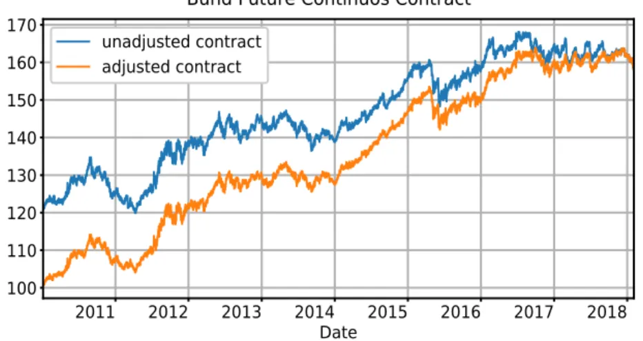
As we can see from figure1.1, the datasets collected do not contain any in-formation about the specific contract to which the price and volume data are referred. The lack of this information considerably complicates the adjust-ment procedure, since we have to figure out by ourselves when the intraday data stop being referred to the expiring and move to the second nearest con-tract. We succeed in getting over this problem by using daily fixing data on both the expiring contract and the second nearest one, that can be collected from other standard data providers. The daily fixing is taken at a given time each date (17:15 CET for Bund futures and 21:00 CET for Treasury futures). Therefore, by comparing the daily data with the intraday data on fixing times taken on the few days before the expiring contract’s last trade date, we can figure out when the transition from the expiring contract to the new one takes place in the intraday price series. Figure 1.2 shows the difference between the unadjusted and the adjusted continuous time series for Bund futures. For further information and considerations about future markets and roll-over events please refers to Schwager and Etzkorn (1984).
2011 2012 2013 2014 2015 2016 2017 2018 Date 100 110 120 130 140 150 160 170 unadjusted contract adjusted contract
Bund Future Continuos Contract
Figure 1.2: Unadjusted and adjusted time series for Bund future prices. The ad-justed time series has been obtained by applying backward multiplicative shifts at each roll event, in order to match the prices of the expiring contract and the second nearest contract.
Euro-Dollar and Bund ones date back to 1999, while the data on Treasury futures are available starting from to 2007: however, we think it is reasonable to limit the analysis from 2010 onward, since there have been major structural changes in market dynamics.
1.5
Problem approach
Machine learning algorithms can be classified according to the amount and type of supervision they get during training. There are three major cate-gories: supervised learning, unsupervised learning, and reinforcement learn-ing.
In supervised learning tasks the training data you feed to the model include the actual realizations of the target variable, which are usually called labels. During training, the model observe both the input data and the correspond-ing target variable responses, and it has to identify the relation between input and target variables: a typical example of a supervised learning al-gorithm is a regression task, where the goal is to predict a target numeric value given a set of features or predictors.
In unsupervised learning, as you might guess, the training data is unlabeled: the system tries to learn by itself, without a teacher that shows the ’correct answer’: for example, unsupervised learning algorithms are used in the field of density estimation in statistics, and in situations that require to summa-rize and explain various key features of the data.
Reinforcement learning is much more different and, in some ways, more com-plex: the learning system, which is called agent in this context, can observe the environment, select and perform actions, and get rewards or penalties in return. The model should identify the optimal strategy, which is called a policy, to get the most reward over time.
For the type of task we are dealing with, the most suitable approaches are those of supervised and reinforcement learning. It is no coincidence that they are adopted by the great majority of similar existing works. All the papers we mentioned in1.2 adopt a supervised learning approach. For pa-pers opting for the reinforcement learning approach see e.g. Dempster and Leemans (2006), Tan et al. (2011), Moody and Saffell (2001).
One could opt for a reinforcement learning framework, since it seems natural to define the profit of the trading strategy to be the reward that the system will try to maximize. The big drawback of this approach is that it would make the training procedure much more burdensome: the network is asked to solve a complex global task, because the strategy’s total return depends on the decisions made over the entire trading period. In order to consider the fees to be paid to implement the selected trading strategy, the objective function cannot be decomposed into temporally independent terms: any ac-tion performed at a given time will influence the optimality of those to be taken later in time.
In a sense, reinforcement learning constitutes a double-edged sword: it rep-resent a more sophisticated and more opportune approach to the problem, because it allows to include in the model additional key factors, such as transaction costs and the impacts that the implemented strategy would have
on the working environment. However, this high modeling power can only be achieved at the expense of a much more complicated learning algorithm. For this reason, we believe it is better, at least initially, to decompose this complex global problem into a sequence of local and easier ones. We adopt a supervised learning approach, where the system outputs a prediction on the asset return on a specific time horizon, rather than an entire trading strategy: we decouple the forecast of expected future return from the choice of the optimal trading strategy conditioned to this forecast, which will be managed separately.
The time horizon over which to make the forecasts is a model parameter to be set externally: in any case, it will be higher with respect to the data sampling frequency. Shortening the forecast horizon reduces the signal-to-noise ratio, which in the case of financial time series is already extremely low. Therefore, it would be more difficult for the network to identify depen-dencies and significant patterns in the data.
On the other hand, if we opt for an excessively long prediction horizon, the trends and patterns characterizing the returns time series will emerge more clearly, but we would limit the trading frequency and, consequently, the op-portunity to profit from what the network learns.
For example, working with price candlesticks sampled on a hourly basis, we make the model predict the asset return over the following 24 hours. Thus, the position we will take on the traded asset once we observe the network forecast, will be re-balanced on a daily basis.
Supervised learning algorithms can be further split into two sub-classes: classification and regression algorithms.
Classification tasks aim at grouping the observations into a set of discrete categories, depending on the values of some input variables, which in ma-chine learning field are usually referred to as features.
Regression algorithms aim at predicting a real valued scalar response, the dependent variable, by identifying the relationship between such a target variable and a set of explanatory features, or independent variables.
Concretely, this translates into choosing whether to predict only the direc-tion of the price movements, implementing a binary classificadirec-tion algorithm in which the two possible categories are ’positive return’ and ’negative re-turn’, or whether to define the neural network so that its output represents the level of expected future return.
There is a lot of disagreement about this point in the existing papers, which are divided more or less equally on the choice between these different ap-proaches. For further lectures about this topic please refer to Leung et al. (2000). This is why we explore both the alternatives: the results of the different experiments are shown in chapter 3.
1.6
Performance evaluation methodology
1.6.1 Common mistakes
The ultimate goal of any machine learning project is to identify, among a wide set of available models, the one that will achieve the best performance in the execution of a particular task. Nevertheless, to accurately estimate the performance that the trained model will have when faced with unseen instances is an error-prone task. In our case this risk is even bigger, because, besides being a typical machine learning issue, overestimating an algorithm’s ability to perform is a common mistake made in trading strategies backtest-ing.
In the field of investment strategy, a backtest is an historical simulation of how a specific strategy would have performed if it would have been adopted over a past period of time. In 2014, a team of quants at Deutsche Bank published a study under the title Seven Sins of Quantitative Analysis, in which they describe the most common oversights to avoid when backtesting a trading strategy. Some of them are listed below:
1. Look-ahead bias, i.e. using information that was not public at the moment the simulated decision would have been made. Backtesting requires to simulate past conditions with sufficient detail: a mistake that might seem trivial, but that we found in some of the similar ex-isting works, is to consider to be synchronous a set of data which are not such.
it is important to keep a precise temporal marking and alignment of the data if they refer to financial assets which are traded on differ-ent exchanges: in the aforemdiffer-entioned works the oversight consists in the alignment of daily closing price for equities which are traded on exchanges with different trading windows during the day, or simply located in different time zones.
2. Survivorship bias, i.e. using as investment universe the current one, hence ignoring that some companies went bankrupt and securities were delisted along the way.
3. Data snooping, namely the eventuality to find a strategy that would have worked well in the past by chance, but will not work as much in the future.
4. Neglect transaction costs: simulating transaction costs is hard because the only way to be certain about that cost would have been to interact with the trading book. Nonetheless, when dealing with high frequency trading, fees and transaction costs play a major role in determining a strategy efficiency. In many papers the authors decide to overlook
these costs, but this approach is way too optimistic in assessing the model ability to generate profits.
5. A further limitation is the impossibility to model how the developed strategies would have affected historical prices.
In the light of the assets universe considered, look-ahead bias represents the greatest risk we face. Survivorship bias does not represent a major issue, since the financial assets we consider are linked to institutions characterized by extremely low default probabilities. Neither estimating and including transaction costs is particularly troublesome, because these financial assets are characterized by bid/ask spreads that are quite constant through time, since they are not very subjected to significant widening during low-liquidity periods. Finally, since we focus on high-liquidity assets, the impact our trad-ing strategy would have had on the historical price series can be neglected.
1.6.2 Machine learning evaluation approach
The standard approach for assessing a machine learning algorithm’s effec-tiveness consists in splitting the overall available data into training, valida-tion and test datasets.
The size of the training set should exceed those of the validation and test set. However, there is no universally valid rule in establishing the relation-ship between those sizes: the guideline is to keep the validation and test sets large enough to allow accurate estimates on the model performances, but at the same time to avoid sacrificing too many samples that could have been used as training instances. Up to a decade ago, when typical datasets were made up of just few thousands of instances, the proportion between training, validation and test instances was kept around 70% − 15% − 15%. With the advent of the Big Data era, the size of the available datasets has grown to the range of millions of instances, and the subsets size ratio has moved in favor of the training set: with such a large number of samples available, it is common practice to establish the proportion between train-ing, validation and test instances to be something like 98% − 1% − 1%. Typically, one considers many different learning algorithms, which are trained on the training set so that they can learn from these data which are the un-derlying relations between the variables of interest.
Considering various machine learning algorithms, and the possible config-urations of each of those algorithms, each one characterized by different values assigned to the model’s hyperparameters3, it is likely to end up train-ing hundreds, if not thousands, of different models.
At this point, the validation data come into play: they are not used to ex-tract further information, but rather to assess which model achieve the best performance when faced with unseen data. The reason why one should not simply select the model that performs best on the training data is that it could have simply adapted itself to the specific instances of that training set: this phenomenon is know as overfitting, and it is arguably the biggest obstacle that whoever is interested in machine learning today has to face. Overfitting is a particularly problematic issue when dealing with certain machine learning algorithms, such as deep artificial neural networks, and when dealing with phenomena characterized by a low signal-to-noise ratio, such as financial returns prediction. Indeed, the mapping between the in-put features and the network’s response goes through a very high number of trainable variables, and it is more likely for a model with such an high modeling power to learn patterns that can be found in the specific training set used, but that are not generally valid. When this occurs, the algorithm
3
In machine learning context, an hyperparameter is a parameter whose value is set externally, before the learning process begins. By contrast, the values of other parameters are derived via the learning procedure.
performs extremely well of the training instances, but it will not be unable to generalize such a good performance on data on which it has not been trained, such as the ones in the validation set.
Ordinary neural networks present thousands of trainable variables and de-grees of freedom, thus preventing the model to overfit the training data might be extremely hard: for this reason, data scientists have introduced a wide array of regularization techniques designed specifically to address this problem.
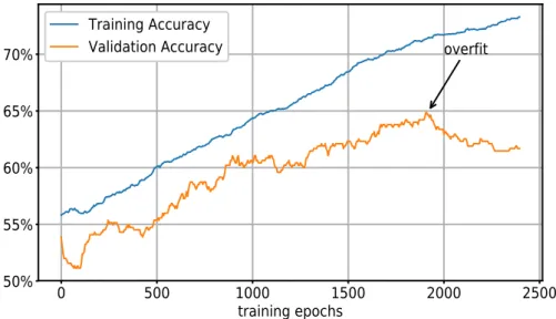
To get an idea of what happens when entering the overfitting regime, it can be helpful to look at figure 1.3. The figure shows the evolution of the accuracy score achieved by an artificial neural network implemented for exe-cuting a binary classification task. We can see the accuracy score computed on both the training and the validation set as the learning phase proceeds.
0 500 1000 1500 2000 2500 training epochs 50% 55% 60% 65% 70% overfit Training Accuracy Validation Accuracy
Figure 1.3: Training and validation accuracy achieved by an artificial neural net-work classifier entering the overfitting regime.
The accuracy on the training set gradually increases as the training epochs4 advance. On the other hand, the validation accuracy evolves in a much less regular way: this behavior is due to the fact that the learning procedure searches for a good fit on the training instances, without caring about the validation ones.
4The term epoch is used in machine learning area to denote a learning cycle over the
entire training set. When the dataset is made up of millions of entries it is common practice to split it up in smaller mini-batches. In order to accelerate the training procedure, the single training iterations works on single mini-batches rather that on the entire dataset. An epochs consists in a sequence of parameters’ updating steps covering all the mini-batches. Refer to2.4.4for further information on this topic.
The validation accuracy presents an increasing trend up to a certain num-ber of training epochs. This means that, at the beginning of the training phase, the network is learning from the training data relations which are generally valid, that are found in the validation set as well. After roughly 1900 epochs, the validation accuracy starts to decrease, an evidence that the neural network has entered the overfitting regime.
The model’s performance on the validation set is typically lower with re-spect to the one achieved during the training phase, but it better reflects the model ability to generalize such a performance on new, unseen data. However, choosing the best model by looking at the results achieved on the validation data introduces a further, more subtle, degree of overfitting: the risk is to select an algorithm rather than another just because the former is, by chance, better suited to the particular validation test used. The perfor-mance observed on the validation set serves as an estimate of the average performance the model will achieve when faced with unseen data: thus, since the validation data are nothing more than a random realization drawn from the probability distribution that governs the phenomenon under analysis, the estimate itself is a random variable subject to stochastic error.
Therefore, it is possible to end up overestimating the out-of-sample effi-ciency of a model that randomly got a higher effieffi-ciency on the validation set. For this reason, one should keep aside a further subset of the overall data, namely the test set, which is not supposed to be used until the very last step, after having selected the alleged best model, in order to get an unbiased estimate of its actual out-of-sample performance.
To give an idea of the typical relative weight of these two different kinds of overfitting, one might train a set of binary classification algorithms which achieve a nearly perfect fit on the training data, let’s say 95% of correctly classified instances, then he selects the model with the highest validation accuracy, let’s say 90%, and eventually he notices a further 0.5% drop in the accuracy score achieved on the test set instances.
1.6.3 Walk forward optimization
In developing anautomated trading system (ATS), we believe that the evalu-ation methodology to be followed to most properly assess the model’s ability to perform, is the one, typical of algorithmic trading, called walk forward optimization (see e.g. Kaastra and Boyd 2001). The idea behind this ap-proach is to simulate what will potentially become the operational trading activity: the overall time span is split into many consecutive windows of training, validation and test periods.
First of all, we have a time window on which the training of different learning models we want to compare is carried out. This is followed by a validation period that allows the selection of the most suitable model and, finally, there
is a test window, which represents the time span in which the actual trad-ing activity would have taken place. The time windows are advanced after each train-validation-test cycle, so that test windows are consecutive and not overlapped.
As explained in the previous paragraph, the training period is more extensive with respect to the validation and test ones, so that the training windows end up being partially overlapped. For example, an appropriate setting we use, is characterized by 40-week long training windows followed by 4-week long validation and test windows: working with hourly sampled price can-dlesticks, this choice entails that each training set consists of roughly 4800 instances, while the validation and testing sets are made up of about 480 instances each.
This optimization mechanism is schematized in figure1.4. This setup
emu-Figure 1.4: Walk forward optimization illustration.
lates a real-world trading situation, where there is a frequent calibration of the model on the most recent time span.
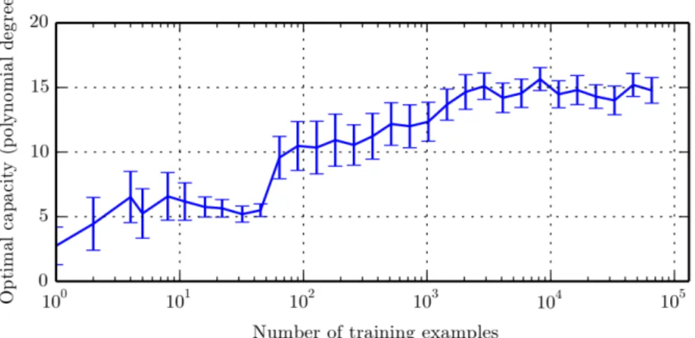
We think that splitting the entire data set into shorter time windows is a reasonable choice. Indeed, a model that fits well over the entire period con-sidered, roughly 8 years of history from 2010 to now, must be able to learn how to manage regime switches and market structure modifications, turn-ing out to be extremely complex and difficult to train. On the other hand, a model that is effective over shorter time periods may have a lower com-plexity and capacity5. By simplifying, it could be said that the short-term model has hard-coded some features that a long-term model should learn.
5
The term capacity, in machine learning, denotes the ability of an algorithm to model complex relationships between inputs and outputs (see e.g. Goodfellow et al., p.111).
1.7
Deep Learning history
The first works on neural networks date back to 1943, when McCulloch and Pitts created a computational model based on mathematics and algorithms called threshold logic.
Further steps were made by Rosenblatt in 1958, who conceived the percep-tron, which constitutes the basic building block on which are based present-day artificial neural network architectures.
Neural network research stagnated after a machine learning research pub-lished in 1972 by Minsky and Papert, where they showed two key issues with the computational machines that processed neural networks. The first was that basic perceptrons were incapable of processing the exclusive-or circuit. The second was that computers did not have enough processing power to ef-fectively handle the computational work required by large neural networks. This caused neural network research to slow until computers achieved far greater processing power.
A key trigger for renewed interest in neural networks and deep learning was Werbos’s (1974) paper on the backpropagation algorithm, which greatly accelerated the training of multi-layer networks. But, at the same time, support vector machines and other much simpler methods, such as linear classifiers, gradually overtook neural networks in machine learning popular-ity.
However, the exponential growth in the available computational power, which has undergone an incredible step forward since the adoption of GPUs for computing purposes in the early 2000s, have finally favored the success of artificial neural networks.
The advent of the Big Data era has allowed artificial neural networks to overcome more traditional machine learning algorithms such as logistic re-gressions, support vector machines and random forests, because the perfor-mance achievable by training a deep neural network improves drastically with the increase in the number of available data.
Further improvements are due to the introduction of a series of training ar-rangements developed in the most recent years, whose purpose is to speed up and optimize the training procedure, by overcoming some of the problems to which neural networks are notoriously subjected, such as the so-called vanishing gradient problem that we discuss in detail in subsection2.1.1. Among these techniques there are different weights initialization schemes6, different choices for the neuron’s activation functions, features pre-processing, batch-normalization and, finally, the development of new iterative minimiza-tion algorithms.
The first stages of deep learning development have been characterized by several troubles and difficulties, which required decades of research to be
6
overcome. However, the innovations became more and more frequent over the years. In the most recent years the number of publications has been growing exponentially, and it is impossible to cite all the progress that has been made. As an example, we cite the work that has captured the most the media’s attention and that has been perceived as the most groundbreaking, namely the project carried out by the AI company DeepMind, which demon-strated a reinforcement learning system that could learn to play almost any Atari game from scratch, eventually outperforming humans in most of them, using only raw pixels as inputs and without any prior knowledge of the rules of the games. This was the first of a series of amazing feats, culminating in March 2016 with the victory of their system AlphaGo against Lee Sedol, the world champion of the game of Go (see Mnih et al. 2013 and Mnih et al. 2015).
Chapter 2
Deep Neural Networks
This chapter illustrates the theoretical principles underlying the functioning of artificial neural networks. Section2.1is focused on the description of feed-forward neural networks (FFNNs), while the concepts and the methodologies introduced in the following sections are more general and can be extended to other types of network architectures. In particular, section2.2describes the main steps in training artificial neural networks. Section2.3 introduces the most popular regularization techniques, which are essential to achieve good performances not only on the specific data on which the learning algorithm is trained, but also on new, previously unseen data. Finally, section2.4ends this chapter by introducing some of the methodologies and techniques which have been developed over the most recent years for optimizing the training procedure of artificial neural networks.
2.1
Feed-Forward Neural Networks
The feed-forward neural network is arguably the type of neural network which is best known to non-professionals. In literature, this network ar-chitecture is often referred to as multi-layer perceptron (MLP) (see e.g. Goodfellow et al., p.5).
It represents the first and simplest kind of artificial neural network con-ceived, and its name arise from the fact that, in this structure, the informa-tion moves only in one direcinforma-tion, forward, from the input layer through the hidden neurons and finally to the output layer. Such a relatively simple and straightforward structure presents multiple advantages. For this reason, the use of these models is still widespread.
Typical FFNNs are characterized by the presence of a quite small number of hidden layers: this number depends on the complexity of the problem that is being addressed, but it remains in the order of a dozen of hidden layers at most (see e.g. Glorot and Bengio 2010). This property makes the learn-ing procedure much less burdensome from a computational point of view,
if compared to that of much deeper architectures, such as state-of-the-art
convolutional neural networks (CNNs) used in computer vision and image recognition applications, which might have more than a hundred hidden lay-ers.
Furthermore, if we represent a FFNN architecture with a computational graph, where each node represents a neuron and each edge represents the information flow between two neurons, we would see that those connections do not form any cycle: the fact that the computations flow in a single di-rection, makes these networks less prone to typical issues which affect the learning process, such as the vanishing gradients problem, which get much worse when dealing with less linear architectures, likerecurrent neural net-works (RNNs).
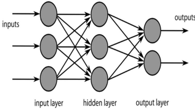
Figure 2.1: Computational graph representing the architecture of a fully-connected1FFNN with a single hidden layer.
Figure2.1depicts the organization of a shallow feed-forward neural network, which is made up of an input layer, a single hidden layer and an output layer. In the general case of deeper FFNNs, the input feature vector is fed to the input layer, it is processed by a series of hidden layers and, finally, the signal goes through a last layer of neurons, the output layer, whose purpose is to reshape the model’s output so that it has the desired format. For example, suppose we are dealing with a binary classification task, and we want to estimate the probability of observing a positive instance given a set of input variables: if the last hidden layer is made up of n neurons, its output is a vector in Rn, therefore the output layer should map Rnin the interval [0, 1]: this can be achieved by choosing an output layer made up of a single neuron with an activation function whose output takes value in the interval [0, 1]. Each layer is made up of a certain number of neurons: the number of neu-rons in the input and output layers depends on the dimension of the input
1
When the input signal of each neuron consists in the whole set of output signals of the neurons in the previous layer, the network is said to be fully-connected