!"#$%&'#()*+%,-#*.(/+#*+#*01+2$1*
3#41&(#5%"(2*+#*.6#%"7%*.(1(#'(#68%*
92&'2*+#*:1/&%1*;1,#'(&1-%*#"*
.6#%"7%*.(1(#'(#68%*
*
*
*
*
*
*
*
*
*
*
*
!"#$#%&"'(#)&"*'+$",-./&$.*0'1#$2,3+,$",2'4#-'.5,'
)/6#-'%/-7,.'8*$/%&"2'
*
*
*
*
*
<%-1(2&%*0&2=>*?=&%5*91'(%-"/2$2**
3#41&(#5%"(2*+#*.6#%"7%*?62"25#68%*
*
*
*
*
*
*
*
:/61*<2''#"#*
;1(>-1*@ABCDBE*
*
*
*
F""2*F661+%5#62*EA@EG@B*
”Alle 3 donne della mia vita e al mio babbo Grazie per avermi so(u)pportato”
Contents
1 Introduction 5
2 VAR and SVAR Models 9
2.1 Basic Assumptions and Properties of VAR Model . . . 9
2.1.1 Stable VAR Model . . . 9
2.1.2 The Moving Average Representation of a VAR Process . . 12
2.1.3 Forecasting and Interval Forecasts . . . 12
2.2 Structural Analysis . . . 14
2.2.1 Granger-Causality, Instantaneous Causality . . . 14
2.2.2 Impulse Response Function . . . 15
2.2.3 Forecast Error Variance Decomposition . . . 16
2.3 Estimation of a VAR model . . . 17
2.3.1 Multivariate Least Square Estimation . . . 17
2.3.2 Testing for Causality . . . 18
2.4 Criteria for VAR order selection . . . 19
2.5 Structural Vector Autoregressions . . . 20
2.5.1 The A-Model . . . 21
2.5.2 The B-Model . . . 21
2.5.3 The AB-Model . . . 22
2.5.4 Estimation of Structural Parameters . . . 22
3 The Theoretical Model 25 3.1 The Model . . . 26
4 Data Analysis 35 4.1 Data Description . . . 35
4.2 Model without VIX index (1985:01-2010:03) . . . 50
4.3 Model with VIX index (1985:01 - 2010:03) . . . 60
4.4 Model without VIX index (1985:01-2008:02) . . . 70
4.5 Model with VIX index (1985:01- 2008:02) . . . 76
4.6 New Policy Uncertainty Index . . . 82
5 Conclusions 87
4 CONTENTS
A Economic Events 89
A.1 The 1987 Stock Market Crash and the Black Monday . . . 89 A.2 Recession of 2001 . . . 90 A.3 The Financial Crisis and Economic Downturn of 2008 and 2009 . 90
B Mathematical Results 93
C FEVD Tables 95
C.1 Model without VIX index (1987:01 - 2008:02) . . . 95 C.2 Model with VIX index (1987:01 - 2008:02) . . . 97
Chapter 1
Introduction
”There’s pretty strong evidence that the rise in uncertainty is a sig-nificant factor holding back the pace of recovery now. [...] research shows that heightened uncertainty slows economic growth, raises un-employment, and reduces inflationary pressures. [...] There’s no question that slow growth, high unemployment, and significant un-certainty are challenges for monetary policy.”
John Williams, President and Chief Executive Officer of the Federal Reserve Bank of San Francisco, FRBSF Economic Letter, January 21, 2013.
The literature on the macroeconomic effects of uncertainty shocks has de-veloped quite fastly in the last few years. This is mainly due to the recent contribution by Bloom (2009), which builds on a previous model by Bernanke (1983) to show that entrepreneurs facing an uncertain economic environment assign a higher value to the option of implementing ”wait-and-see” strategies which lead to a pause in investments. As a consequence, economic activities go bust in the short run, which consequences involving prices and monetary policy setting.
Bloom (2009) established that volatility shocks are strongly correlated with other measures of uncertainty, like the cross-sectional spread of firm- and industry-level earnings and productivity growth. Moreover, he noticed that the uncer-tainty is also a ubiquitous concern of policymakers, as the opening statement of this thesis also confirms.
After Bloom’s article, there has been a number of contributions in this litera-ture. Fernandez-Villaverde et al. (2011) set up a theoretical model to investigate whether all the increased uncertainty about mix and timing of fiscal austerity has had a detrimental impact on current business conditions through its effect on expectations and behavior of households and firms. They find that the fiscal volatility shocks reduce economics activity: aggregate output, consumption and investment; the increase in fiscal policy uncertainty of two standard deviation has an effect similar to 25-basis-point innovation in federal funds rate and finally
6 CHAPTER 1. INTRODUCTION that heightened fiscal policy uncertainty is ”stagflationary”: it creates inflation while output falls.
Recent empirical VAR-based investigations confirm that shocks to uncer-tainty are an important driver behind macroeconomic fluctuations (Bloom (2009), Baker, Bloom and Davis (2013), Leduc and Liu (2013), Mumtaz and Theodor-idis (2012)). Typically, uncertainty matters in a context in which risk matters. In particular, some recent research has pointed out the time-dependence of risk aversion and discount factors and risk aversion tends to be high during phases of stress like recessions. In particular, Leduc and Liu (2013) show that, in an economy featuring real matching frictions in the labor market and using a dynamic stochastic general equilibrium model, uncertainty shocks act as ”de-mand” shocks, in that they increase unemployment and decrease inflation. This is so because positive uncertainty shocks negatively affect potential output and this occurs because firms pause hiring new workers when uncertainty hits the economy due to lower expected value of a filled vacancy. As a consequence, firms post a lower number of vacancies, so inducing a drop in the job finding rate and an increase in unemployment rate.
Mumtaz and Theodoridis (2012) propose a model in which nominal frictions affecting wage and price re-setting induce a reaction to uncertainty shocks sim-ilar to the one that occurs when supply shocks hit the economy. This is due to the fact that risk-averse workers ask for a wage-premium to ensure themselves against the scenario which may be seen them called to work extra-hours at a predetermined wage (due to wage stickiness). In reaction to workers’ request of a higher wage, firms increase their prices to lower the burden of real wages on their marginal costs. As a result, uncertainty shocks act as inflationary, supply shocks in their model.
Baker, Bloom and Davis (2013) investigate the role of economic policy un-certainty shocks. They create a new economic policy unun-certainty index based on a variety of components (news, forecasters’ disagreement), and employ it in a VAR context to investigate the effects of exogenous variations of uncertainty on the U.S. macroeconomic environment. They find that an increse in uncertainty comparable to the one recorded in the U.S. after the acceleration of the financial crises may have been an important driver of the economic downturns observed in 2009 and 2010.
This thesis aims at contributing to this literature by asking the following question: Does economic policy uncertainty influence the labor market dynamics in the United States? To tackle this question, we use actual U.S. data from the first quarter of 1985 to the third quarter of 2010 and estimate a VAR including labor market’s variables (the unemployment rate, the job creation’s rate, the job destruction’s rate, the job finding rate), the policy uncertainty index `a la Baker et al (2013), the Federal Funds rate, the inflation rate, the output gap and the VIX index related to the U.S. economy. After estimating our VAR, we make extensive use of the impulse response and variance decomposition analyses to pin down the role played by economic policy uncertainty shocks in affecting the U.S. labor market dynamics.
7 policy uncertainty indicator on unemployment and other-labor market related variables. This is true even when controlling for alternative, broader volatil-ity indicators like the VIX, measures of the business cycle like real GDP, and indicators of monetary policy stance like the nominal interest rate and infla-tion. Differently, we find the reaction of inflation to be quantitatively mild and, above all, statistically insignificant for most of the horizons following our simulated uncertainty shock. Our results corroborate those proposed by Leduc and Liu (2013) on the relevance of uncertainty shock as far as the real side of the economy is concerned. Differently, we find mild evidence at best on such shocks as being behind inflation dynamics in the United States. Therefore, we cast some doubts on the robustness of Leduc and Liu’s results as far as the uncertainty-inflation relationship is concerned.
This thesis is structured as follows. In the first section, we introduce the VAR theory and how to use it and all the functions useful for the analysis (the impulse response function, the causality test, etc). In the second section, we explain the theoretical model `a la Leduc and Liu (2013) to have a theoretical benchmark to interpret the impulse response functions of interest. The third section proposes our VAR analysis based on the U.S. data from the first quarter of 1985 to the third quarter in 2010. First of all, we present and describe all the variables that we use in the models and we analyse two different models, one with the VIX index, which is a key measure of market expectations of near-term volatility conveyed by S&P 500 stock index option prices, and the other without it. In practice we try to study, using the VIX index, if the stock market influences the economic policy uncertainty and if there are possible new relationships between the labor market variables and the economic policy uncertainty shocks. Since we identify some clear outliers during the 2008-2009 financial crisis, we move to an analysis focusing on pre-crisis data. Then, we introduce in our investigation the policy uncertainty index `a la Baker, Bloom, and Davis (2013) and check if there are some differences respect to the other previous models in terms of impulse response function and variance decomposition. In the last section, we conclude our thesis and in the appendix we explain some important economic events related to our analysis, some mathematical proofs and some FEVD tables.
Chapter 2
VAR and SVAR Models
In this chapter we introduce the stationary finite order vector autoregressive (VAR) model, it is one of the most successful, flexible and easy to use models for the analysis of multivariate time series. It is a natural extension of the univariate autoregressive model to dynamic multivariate time series. As Sims (1980) used, the VAR model has proven to be especially useful for describing the dynamic behavior of economic and financial time series and for the forecasting and structural analysis.
In addition to data description and forecasting, the VAR model is also used for structural inference and policy analysis. In structural analysis, certain as-sumption about the causal structure of data under investigation are imposed, and the resulting causal impacts of unexpected shocks or innovations to spec-ified variables on the variables in the model are summarized. These causal impacts are usually summarized with impulse response function and forecast error variance decomposition.
The model of interest is assumed to be known, but this assumption is not true in the real life, and it helps us to see the problems related to VAR models without contamination by estimation and specification issues. In the following section, we describe the principal properties and the important functions of a VAR model.
2.1
Basic Assumptions and Properties of VAR
Model
2.1.1
Stable VAR Model
We start our analysis from the VAR(p) model (Vector Autoregressive model of order p)
yt= ν + A1yt−1+ · · · + Apyt−p+ ut, t = 0,±1, ±2, . . . (2.1)
10 CHAPTER 2. VAR AND SVAR MODELS
where yt= (y1t, . . . , yKt)� is a (K × 1) random vector, the Ai are fixed (K × K)
coefficient matrices, ν = (ν1, . . . , νK)� is a fixed (K × 1) vector of intercept
terms allowing for the possibility of a nonzero mean E(yt). Than the ut =
(u1t, . . . , uKt)� is a (K × 1) vector, called white noise or innovation process,
such that E(ut) = 0 and
E(utus) =
� Σu, if t = s
0, if t �= s
where the Σu is assumed to be nonsingular (invertible)
To understand the general VAR model of order p described by (2.1), we consider the VAR(1) model:
yt= ν + A1yt−1+ ut. (2.3)
If this generation mechanism starts at some time t = 1, we have:
y1= ν + A1y0+ u1 y2= ν + A1y1+ u2= ν + A1(ν + A1y0+ u1) + u2 = (IK+ A1)ν + A21y0+ A1u1+ u2 ... (2.4) yt= (IK+ A1+ · · · + At1−1)ν + At1y0+ t−1 � i=0 Ai 1ut−i ...
The vectors y1, . . . , ytare uniquely determined by y0, u1, . . . , utand also the joint
distribution of y1, . . . , ytis determined by the joint distribution of y0, u1, . . . , ut.
We consider the VAR(1) process and using the (2.4) we have
yt= ν + A1yt−1+ ut = (IK+ A1+ · · · + Aj1)ν + A j+1 1 yt−j−1+ j � i=0 Ai1ut−i.
If all eigenvalues of A1 have modulus less than 1, the sequence Ai1, i = 0, 1, . . .
is absolutely summable1and we have also that
(IK+ A1+ · · · + Aj1)ν −−−→
j→∞ (IK− A1) −1ν.
1A sequence of (K× K) matrices {A
i = (amn,i)}, i = 0, ±1, ±2, . . . is absolutely
summable if each sequence{amn,i}, m, n = 1, . . . , K; i = 0, ±1, ±2 is absolutely summable.
{Ai} is absolutely summable if the sequence {||Ai||} is summable, where
||Ai|| = „X m X n a2 mn,i «1/2
2.1. BASIC ASSUMPTIONS AND PROPERTIES OF VAR MODEL 11
Furthermore, Aj+1
1 converges to zero rapidly as j → ∞ and so we ignore the
term Aj+1
1 yt−j−1 in the limit. Also if all eigenvalues of A1 have modulus less
than 1, then ytis the well-defined stochastic process:
yt= µ + ∞ � i=0 Ai 1ut−i, t = 0,±1, ±2, . . .
where µ := (IK− A1)−1ν. The distribution and the joint distributions of the
yt’s are uniquely determined by the distributions of the utprocess. We calculate
the first and the second moment:
E[yt] = µ ∀t Γy(h) := E[(yt− µ)(yt− µ)�] = ∞ � i=0 Ah+i1 ΣuAi � 1.
Definition 1. We call a VAR(1) process stable if all eigenvalues of A1 have
modulus less than 1 and it is equivalent to:
det(IK− A1z)�= 0 for|z| ≤ 1. (2.5)
We extend this discussion to a VAR(p) process, in fact a VAR(p) corresponds to a Kp-dimensional VAR(1): Yt= ν + AYt−1+ Ut (2.6) where: Yt:= yt yt−1 ... yt−p+1 ν := ν 0 ... 0 A := A1 A2 · · · Ap−1 Ap IK 0 · · · 0 0 0 IK 0 0 ... ... ... ... 0 0 · · · IK 0 Ut:= ut 0 ... 0
where Yt, ν and Utare (Kp × 1) vectors and the matrix A is (Kp × Kp).
Definition 2. The VAR(p) process is stable if
det(IKp−Az) �= 0 for|z| ≤ 1 ⇐⇒ det(IK−A1z−· · ·−Apzp) �= 0 for|z| ≤ 1.
A stochastic process is stationary if its first and second moments do not
change with time t. So a stochastic process ytis stationary if
E(yt) = µ for all t (2.7)
12 CHAPTER 2. VAR AND SVAR MODELS
From (2.7) all the yt have the same finite mean vector µ and from (2.8) the
autocovariances of the process do not depend on t but only on h that is the lag period.
Proposition 1. If a VAR process is stable, then it is stationary.
2.1.2
The Moving Average Representation of a VAR
Pro-cess
The VAR(p) process Yt have also an other representation under the stability
assumption: Yt= µ + ∞ � i=0 Ai Ut−i (2.9)
and this form is called the Moving Average (MA) representation, where Yt is
expressed in terms of past and present errors or innovation vectors Utand the
mean term µ. This representation of yt can be found by using the matrix
(K × Kp), J := [IK: 0 : · · · : 0]: yt= JYt= Jµ + ∞ � i=0 JAiJ�JUt−i= µ + ∞ � i=0 φiut−i (2.10)
where µ := Jµ, φi := JAiJ�, ut = JUt and the Ai and φi are absolutely
summable. We can also calculate the mean and the autocovariances
E(yt) = µ Γy(h) = E[(yt− µ)(yt−h− µ)�] = E�� h−1 � i=0 φiut−i+ ∞ � i=0 φh+iut−h−i ���∞ i=0 φiut−h−i ��� =�∞ i=0 φh+iΣuφ�i. (2.11)
2.1.3
Forecasting and Interval Forecasts
In this section we discuss predictors based on a VAR process, we want to know
the future values of variables y1, . . . , yK.
Forecasting
First we define an information set, called Ωt, containing the available
informa-tions in period t and may contain also the past and the present variables of the
system under consideration: Ωt= {ys|s ≤ t}, where ys = (y1s, . . . , yKs)�. The
2.1. BASIC ASSUMPTIONS AND PROPERTIES OF VAR MODEL 13 of periods into the future is the forecast horizon and the predictor h periods ahead is called the h-step predictor.
Suppose yt= (y1t, . . . , yKt) is a K-dimensional stable VAR(p) process, then
the minimum mean squared errors (MSE) predictor for forecast horizon h at forecast origin t is the conditional expected value:
Et(yt+h) := E(yt+h|Ωt) = E(yt+h|{ys|s ≤ t}). (2.12)
This predictor minimizes the MSE of each component of yt, if ¯yt(h) is h-step
predictor at origin t,
M SE[ ¯yt(h)] = E[(yt+h− ¯yt(h))(yt+h− ¯yt(h))�]
≥ MSE[Et(yt+h)] = E[(yt+h− Et(yt+h))(yt+h− Et(yt+h))�]. (2.13)
The optimality of the conditional expectation can be seen by noting that:
M SE[ ¯yt(h)] = MSE[Et(yt+h)] + E{[Et(yt+h) − ¯yt(h)][Et(yt+h) − ¯yt(h)]�}
where the second element of the right-hand side is null, so we have that:
Et(yt+h) = ν + A1Et(yt+h−1) + · · · ApE(yt+h−p) (2.14)
is the optimal h-step predictor of a VAR(p) process such that Et(ut+h) = 0 for
h > 0.
Interval Forecasts
We have to make an assumption about the distributions of the ytor the ut. We
have to consider that yt, yt+1, . . . , yt+h have a multivariate normal distribution
for any t and h and also that ut are multivariate normal, ut∼ N(0, Σu) and ut
and usare independent for s �= t. Under these assumptions, the forecast errors
are also normally distributed as linear transformations of normal vector.
yt+h(h) − yt(h) ∼ N(0, Σy(h)) ⇒
yk,t+h− yk,t(h)
σk(h) ∼ N(0, 1)
(2.15)
where yk,t(h) is the k-th component of yt(h) and σk(h) is the square root of the
k-th diagonal element of Σy(h). Let’s z(α) the upper α100 percentage point of
the normal distribution, we get:
1 − α = P r�−z(α/2)≤
yk,t+h− yk,t(h)
σk(h) ≤ z(α/2)
�
and the (1 − α)100% interval forecast, h periods ahead, for the k-th component
of ytis
14 CHAPTER 2. VAR AND SVAR MODELS
2.2
Structural Analysis
We use the VAR models to analyze the relationships between variables of interest and we start our analysis from the two different definitions of causality, Granger and instantaneous.
2.2.1
Granger-Causality, Instantaneous Causality
Granger-Causality
The concept of causality (Granger 1969) is that a cause can not come after
the effect. Suppose that Ωt is the information set containing all the relevant
information in the universe and including period t. Let zt(h|Ωt) be the optimal
(minimum MSE) h-step predictor of the process zt at origin t based on the
information in Ωt. The corresponding forecast MSE will be denoted by Σz(h|Ωt).
The process xt is said to cause ztin Granger’s sense if
Σz(h|Ωt) < Σz(h|Ωt\ {xs|s ≤ t}) for at least one h = 1, 2, . . . (2.16)
where the Ωt\{xs|s ≤ t} is the set containing all the relevant information in the
universe except for the information in the past and present of the xtprocess. If
xtcauses ztand vice versa, the process (zt�, x�t)� is called feedback system.
If we have a VAR process yt, written in the canonical MA representation:
yt= µ +
∞
�
i=0
φiut−i= µ + φ(L)ut, φ0= IK (2.17)
where ut is a white noise process with nonsingular covariance matrix Σu. We
write the VAR process as
yt= � zt xt � =�µ1 µ2 � +�φ11(L) φ12(L) φ21(L) φ22(L) � � u1t u2t � . (2.18)
Proposition 2. Let yt be a VAR process as in 2.18, then zt is not
Granger-caused by xt if and only if φ12= 0.
Corollary 1. If we take a stationary and stable VAR(p) process:
yt= � zt xt � =�µ1 µ2 � +�A11,1 A12,1 A21,1 A22,1 � � zt−1 xt−1 � +· · ·+�A11,p A12,p A21,p A22,p � � zt−p xt−p � +�u1t u2t �
we have that zt is not Granger-caused by xt if and only if A12,i = 0 for i =
1, . . . , p.
Instantaneous Causality
There is also another kind of causality, called instantaneous causality between
ztand xtif
2.2. STRUCTURAL ANALYSIS 15
In period t, adding xt+1to the information set Ωthelps to improve the forecast of
zt+1and also if there is the instantaneous causality between ztand xt, then there
is also instantaneous causality between xt and zt. If we take the nonsingular
innovation covariance matrix
Σu=
�Σ
11 Σ12
Σ21 Σ22
�
where Σu= P P� and P is a lower triangular nonsingular matrix with positive
diagonal elements. We can write our VAR model:
yt= µ + ∞ � i=0 φiP P−1ut−i= µ + ∞ � i=0 Θiwt−i (2.19)
where Θi := φiP and wt := P−1ut is white noise with covariance matrix:
Σw = P−1Σu(P−1)� = IK and the wthave uncorrelated components and they
are called orthogonal residuals or innovations.
Proposition 3. Using the Σu matrix, there is no instantaneous causality
be-tween ztand xt if and only if
Σ12= E(u1tu�2t) = 0. (2.20)
2.2.2
Impulse Response Function
We have seen that the Granger-causality may not tell us all the things about the interactions between two or more variables. In this case it’s better knowing the response of one variable to an impulse in another variable in a system, and it’s important because we can see the effect of an exogenous shock or innovation in one of the variables on all the other variables. We will study the causality by finding the effect of an exogenous shock or innovation in one of the variables on the others.
Using the Granger-causality, we have that an innovation in variable k has no effect on the other variables if the former variable does not Granger-cause the set of remaining variables, and using the mathematical functions, we have:
φjk,i= 0 for i = 1, 2, . . . ⇐⇒ φjk,i= 0 for i = 1, . . . , p(K − 1)
and we know that ytis a K-dimensional stable VAR(p) process and j �= k. The
meaning is that if the first pK − p responses of variable j to an impulse in variable k are zero, all the following responses must also be zero.
We use the MA coefficient matrices for searching the impulse and accumulate
responses. In fact the Ψn:= �ni=0Φicontains the accumulated responses over n
periods to a unit shock in the k-th variable of the system, and this quantities are called interim multipliers. The total accumulated effects for all future periods
are obtained by summing the MA coefficient matrices. Ψ∞:= �∞
i=0Φiis called
the matrix of long-run effects or total multipliers and it is obtained by:
16 CHAPTER 2. VAR AND SVAR MODELS We have shocks that occur in more variables and the correlation of the error terms may indicate that a shock in one variables is likely to be accompanied by a shock in another variable. If the correlation is null, then we have an orthogonal response impulse function. Also we use the MA representation:
yt=
∞
�
i=0
Θiwt−i (2.21)
where the components of wt = (w1t, . . . , wKt)� are uncorrelated and have unit
variance, Σw= IK and (2.21) is obtained by decomposing2 Σu = P P�, where
P is a lower triangular matrix and Θi = ΦiP and wt = P−1ut and this says
that a change in one component of wt has no effect on the other components
because the components are orthogonal (uncorrelated). The elements of the
Θiare interpreted as responses of the system to such innovations and the jk-th
element of Θiis assumed to represent the effect on variable j of a unit innovation
in the k-th variable that has occurred i periods ago.
If we want to verify that there is no response at all of one variable to an
impulse in one of the other variables, we must use the matrix Θiand its elements
θjk,i. In fact, if ytis a K-dimensional stable VAR(p) process for j �= k:
θjk,i= 0 for i = 0, 1, 2, . . . ⇐⇒ θjk,i= 0 for i = 0, 1, . . . , p(K − 1).
There is a problem related to the ordering of the variables, because we can not determined it. The ordering has to be such that the first variable is the only one with a potential immediate impact on all other variables. The second
variable may have an immediate impact on the last K − 2 components of ytbut
not on y1t and so on.
2.2.3
Forecast Error Variance Decomposition
The forecast error variance decomposition (FEVD) answers the following
ques-tion: what portion of the variance of the forecast error in predicting yi,t+h is
due to the structural shock wi?
We take the MA representation of a VAR process with orthogonal white noise innovations: yt= µ + ∞ � i=0 Θiwt−i (2.22)
with Σw= IK, the error of the optimal h-step forecast is:
yt+h− yt(h) = h−1 � i=0 Φiut+h−i= h−1 � i=0 Θiwt+h−i.
2The Choleski Decomposition says that if A is a positive definite (m× m) matrix, then
there exists a lower (upper) triangular matrix P with positive main diagonal such that: P−1AP�−1= Im or A = P P�.
2.3. ESTIMATION OF A VAR MODEL 17
Let’s θmn,i the mn-th element of Θi, the h-step forecast error of the j-th
com-ponent of yt is: yj,t+h− yj,t(h) = K � k=1 (θjk,0wk,t+h+ · · · + θjk,h−1wk,t+1).
Then we have that wk,t’s are uncorrelated and have unit variances, the MSE of
yj,t(h) is: M SE(yj,t(h)) = K � k=1 (θ2 jk,0+ · · · + θjk,h−12 )
and the contribution of innovations in variable k to the forecast error variance of variable j θjk,02 + · · · + θjk,h2 −1= h�−1 i=0 (e� jΘiek)2.
Using all these equations, we have the proportion of the h−step forecast error variance of variable j: wjk,h= h−1 � i=0 (e� jΘiek)2/M SE[yj,t(h)]. (2.23)
2.3
Estimation of a VAR model
In this section we assume that our VAR(p) process is stationary and stable:
yt= ν + A1yt−1+ · · · + Apyt−p+ ut (2.24)
and we assume that all the coefficients ν, A1, . . . , Ap, Σu are unknown and we
use this time series data to estimate the coefficients.
2.3.1
Multivariate Least Square Estimation
We analyze the multivariate least squares (LS) estimation, we consider our VAR(p) model and we define:
Y := (y1, . . . , yT) (K × T ) B := (ν, A1, . . . , Ap) (K × (Kp + 1)) Zt:= (1, yt, . . . , yt−p+1)� ((Kp + 1) × 1) Z := (Z0, . . . , ZT−1) ((Kp + 1) × T ) U := (u1, . . . , uT) (K × T ) y := vec(Y ) (KT × 1) β := vec(B) ((K2p + K) × 1) b := vec(B�) ((K2p + K)× 1) u := vec(U ) (KT × 1)
18 CHAPTER 2. VAR AND SVAR MODELS where vec(A) = a1 ... an
trasforms an (m × n) matrix A into an (mn × 1) vector by stacking the columns. We have the VAR(p) model for t = 1, . . . , T in the
compactly formula3:
Y = BZ + U or vec(Y ) = (Z�⊗ IK)vec(B) + vec(U) (2.25)
or y = (Z�⊗I
K)β+u. Remind that Σu= IT⊗Σu, we can obtain the multivariate
LS estimation (or also the generalized least squares (GLS) estimation) of β by minimize the following function of β:
S(β) = u�(IT ⊗ Σu)−1u = [y− (Z�⊗ IK)β]�(IT ⊗ Σ−1u )[y − (Z�⊗ IK)β]
= y�(I
T ⊗ Σ−1u )y + β�(ZZ�⊗ Σ−1u )β − 2β�(Z ⊗ Σ−1u )y. (2.26)
Then using the first order condition, deriving the function S(β) respect to β and equating it at zero we have:
ˆ
β = ((ZZ�)−1⊗ Σu)(Z ⊗ Σ−1u )y = ((ZZ�)−1Z⊗ IK)y. (2.27)
The LS estimator is the same that we can obtain by the OLS regression and we can also write this estimator in a different form:
vec( ˆB) = ((ZZ�)−1Z⊗ IK)vec(Y ) = vec(Y Z�(ZZ�)−1) ⇐⇒ ˆB = Y Z�(ZZ�)−1.
We consider the LS estimator and we define: Γ := plimZZ�/T , so we have
the following:
Proposition 4. Let yt be a stable, K-dimensional VAR(p) process with
stan-dard white noise residuals, ˆB = Y Z�(ZZ�)−1 is the LS estimator of the VAR
coefficient B and plim ˆB = B:
√
T ( ˆβ− β) =√T vec( ˆB− B)−→ N(0, Γd −1⊗ Σu). (2.28)
2.3.2
Testing for Causality
If we want to test the Granger-causality, we need to test zero constraints for the coefficients:
H0: Cβ = c against H1: Cβ �= c
3Let A = (a
ij) and B = (bij) be (m× n) and (p × q), the (mp × nq) matrix
A⊗ B := 2 6 4 a11B . . . a1nB .. . ... am1B . . . amnB 3 7 5
2.4. CRITERIA FOR VAR ORDER SELECTION 19
where C is an (N × (K2p + K)) matrix of rank N and c is an (N
× 1) vector.
Using the estimator for Σu and Γ we find the following statistic:
λW = (C ˆβ− c)�
�
C((ZZ�)−1⊗ ˆΣu)C�
�−1
(C ˆβ− c)−→ χd 2(N).
Otherwise if we want to testing the instantaneous causality, we need to test
zero restrictions for the σ = vech(Σu): 4
H0: Cσ = 0 against H1: Cσ �= 0.
We have the following statistic:
λW = T ˜σ�C�[2CD+K(˜Σu⊗ ˜Σu)D�+KC�]−1C ˜σ
d
−→ χ2(N)
where ˜Σu is a plausible estimator and is asymptotically equivalent to ˆΣu.Then
D+K is the Moore-Penrose5 (generalized) inverse of the duplication matrix DK
and C is an (N × K(K + 1)/2) matrix of rank N.
If we use the Choleski decomposition of Σuand the lower triangular matrix
P , we note that instantaneous noncausality implies zero elements of Σuand so
also of P and we have the following hypothesis:
H0: Cvech(P ) = 0
and the statistics:
λW = T vech( ˜P )�C�[C ˆ¯H ˆΣσ˜Hˆ¯�C�]−1Cvech( ˜P )
d
−→ χ2(N)
where ¯H = [LK(IK2 + KKK)(P ⊗ IK)L�K]−1, then Kmn is the commutation
matrix defined such that vec(G) = Kmnvec(G�) for any matrix G and LK is
the elimination matrix defined such that vech(F ) = LKvec(F ) for any matrix
F and finally the ˜P and ˜σ are derived from the asymptotic distribution.
2.4
Criteria for VAR order selection
We use different criteria for choosing the VAR order selection: FPE,AIC, HQ and SC.
i) The Akaike’s Final Prediction Error criterion, called FPE, was designed as an estimator of the prediction error and it is strongly biased in the finite sample case, i.e, in the case that the number of given data is not large compared to the maximum candidate order. The criterion is:
FPE(m) = det�T + Km + 1 T T T− Km − 1Σ˜u(m) � =�T + Km + 1 T− Km − 1 �K det ˜Σu(m).
4The vech operator takes only the elements below and on the main diagonal of a square
matrix. If A is an (m× m) matrix, vech(A) is an m(m + 1)/2 vector.
5A matrix B is called Moore-Penrose (generalized) inverse of A if its satisfies the following
20 CHAPTER 2. VAR AND SVAR MODELS The VAR order estimate is obtained as that value for which the two forces are balanced optimally.
ii) The Akaike’s Information Criterion, called AIC, is based on the minimiza-tion of the forecast MSE, it is an objective measure of model suitability which balances model fit and model complexity. For a VAR(m) process the criterion is:
AIC(m) = ln |˜Σu(m)| +
2
T(number of freely estimated parameters)
= ln |˜Σu(m)| +
2mK2
T .
iii) The Hannan-Quinn Criterion, called HQ, is a consistent criterion and can be applied to regression model and for the VAR(m) process the criterion is:
HQ(m) = ln |˜Σu(m)| +
2 ln ln T
T (# freely estimated parameters)
= ln |˜Σu(m)| +
ln T
T mK
2.
iv) The Bayesian Information Criteria or Schwarz Criteria, called SC or BIC, is a consistent criterion and it focuses on the Bayesian arguments and for the VAR(m) process the criterion is:
SC(m) = ln |˜Σu(m)| +
ln T
T (# freely estimated parameters)
= ln |˜Σu(m)| +
ln T
T mK
2.
In the last three different criteria we choose the order estimated ˆp so that it minimizes the value of the criteria. In the last two criteria we also substitute the non negative function of the AIC criterion with the logarithm.
Proposition 5. Let yTM+1, . . . , yo, y1, . . . , yT be any K-dimensional multiple
time series and suppose that VAR(m) models, m = 0, 1, . . . , M are fitted to
y1, . . . , yT. Then we have the following results:
ˆp(SC) ≤ ˆp(AIC) if T ≥ 8 ˆp(SC) ≤ ˆp(HQ) for all T ˆp(HQ) ≤ ˆp(AIC) if T ≥ 16.
2.5
Structural Vector Autoregressions
We define our K-dimensional stationary, stable VAR(p):
2.5. STRUCTURAL VECTOR AUTOREGRESSIONS 21
where yt is a (K × 1) vector of observable time series variables, Aj is a (K ×
K) matrices and ut is a K-dimensional white noise, with ut ∼ (0, Σu). In
this section we analyze the Structural Vector Autoregression, called SVAR and the restrictions that we do to identify the relevant innovations and impulse responses.
The SVAR models are usually used to study the average response of the model variables to a given one-time structural shock, they allow the construction of forecast error variance decompositions that quantify the average contribution of a given structural shock to the variability of the data.
The SVAR models use nonsample information in specifying unique innova-tions and unique impulse responses, we introduce three different SVAR models: the A-Model, the B-Model and the AB-Model.
2.5.1
The A-Model
If we want to find a model with instantaneously uncorrelated residuals, we have to model the instantaneous relations between the observable variables directly. We consider a structural form model:
Ayt= A∗1yt−1+ · · · + A∗pyt−p+ εt (2.29)
where A∗
j := AAj (j = 1, . . . , p) and εt := Aut ∼ (0, Σε = AΣuA�) The
restrictions have to be such that the system of equations has an unique solution:
A−1Σ
εA�−1= Σu and CAvec(A) = cA (2.30)
where CAvec(A) = cA are the arbitrary restrictions on A and CAis a 12K(K +
1) × K2) selection matrix and c
A is a suitable 12K(K + 1)× 1) fixed vector.
Proposition 6 (Identification of the A-Model).
Let Σεbe a (K×K) positive diagonal matrix and let A be a (K×K) nonsingular
matrix. Then for a given symmetric, positive definite (K × K) matrix Σu, an
(N × K2) matrix C
A and a fixed (N × 1) vector cA, the system of equations in
(2.30) has a locally unique solution for A and the diagonal elements of Σε if
and only if rk −2D + K(Σu⊗ A−1) D+K(A−1⊗ A−1)DK CA 0 0 Cσ = K2+1 2K(K + 1)
where the DK is the duplication matrix and Cσ is a selection matrix which
selects the elements of vech(Σε) below the main diagonal.
2.5.2
The B-Model
If we want to identify the structural innovations �t directly from the forecast
errors or reduced form residuals ut, we have to think of the forecast errors as
22 CHAPTER 2. VAR AND SVAR MODELS
ut = Bεt and Σu = BΣεB� and we assume that εt ∼ (0, IK). We have the
following restrictions:
Σu= BB� and CBvec(B) = 0 (2.31)
where CBis an (N × K2) selection matrix.
Proposition 7 (Local Identification of the B-Model).
Let B be a nonsingular (K × K) matrix. Then for a given symmetric, positive
definite (K × K) matrix Σu and an (N × K2) matrix CB, the system in (2.31)
has a locally unique sollution if and only if:
rk�2DK+(B × Ik)
CB
�
= K2.
2.5.3
The AB-Model
We consider both types of restrictions of the two previously models and we
have a AB-Model: Aut = Bεt and εt ∼ (0, IK). In this case a simultaneous
equations system is formulated for the errors of the reduced form model rather than the observable variables directly. We write the following two restrictions for our model:
Σu= A−1BB�A�−1; CAvec(A) = cA and CBvec(B) = cB. (2.32)
Proposition 8 (Local Identification of the AB-Model).
Let A and B be nonsingular (K × K) matrices. Then, for a given symmetric,
positive definite (K × K) matrix Σu, the system of equations in (2.32) has a
locally unique solution if and only if rk −2D + K(Σu⊗ A−1) 2D + K(A−1B ⊗ A−1) CA 0 0 CB = 2K2.
2.5.4
Estimation of Structural Parameters
We used a AB-model and the A− and B−models are special cases of the AB−model. We want to estimate the following SVAR model:
Ayt= AAYt−1+ Bεt (2.33)
where the Y�
t−1 := [yt−1� , . . . , yt−p� ], A := [A1, . . . , Ap] and εt is assumed to
be white noise with covariance matrix IK, εt ∼ N(0, IK). The reduced form
residuals corresponding to (2.33) have the form ut= A−1Bεtand we have that
2.5. STRUCTURAL VECTOR AUTOREGRESSIONS 23
We have that the log-likelihood function for a sample y1, . . . , yT is seen to
be:
ln l(A, A, B) = −KT2 ln 2π − T2 ln |A−1BB�A�−1|
−12tr{(Y − AX)�[A−1BB�A�−1]−1(Y − AX)}
=constant +T
2 ln |A|2−
T
2 ln |B|2
−12tr{A�B�−1B−1A(Y − AX)(Y − AX)�}
where Y := [y1, . . . , yT], X := [Y0, . . . , YT−1] and we have the following two
rules: |A−1BB�(A−1)�| = |A−1|2
|B|2= |A|−2|B2
| and tr(V W ) = tr(W V ) We maximize the log-likelihood function with respect to A and we obtain:
ˆ
A = Y X�(XX�)−1. (2.34)
If only just-identifying restrictions are imposed on the structural parameters,
we have for the ML estimator of Σu,
˜
Σu= T−1(Y − ˆAX)(Y − ˆAX)� = ˜A−1B ˜˜B�A˜�−1.
Otherwise if over-identifying restrictions have been imposed on A and/or B, the corresponding estimator for
˜
Σr
u:= ˜A−1B ˜˜B�A˜�−1
will differ from ˜Σu.
We see that both the impulse response function and the forecast error vari-ance decomposition are based on the structural innovations and we have that the impulse response coefficients are obtained from the matrices:
Chapter 3
The Theoretical Model
In this chapter we introduce a theoretical model for the analysis of our problem, this model is related to the unemployment and the job finding and the policy uncertainty. Our VAR analysis is justified by a recent work by Leduc and Liu (2012)[18], who work out a structural DSGE model with labor market and nominal frictions to investigate the effects of uncertainty shocks on labor market dynamics.
To study the macroeconomic effects of uncertainty we introduce a stylized Dynamic Stochastic General Equilibrium (DSGE) model with labor market search frictions. DSGE model starts specifying a number of economic agents (like households, firms, governments) and embodying them with behavioral as-sumptions, like the maximization of an objective function (utility).
First the economists assume sources of shocks to model (shocks to produc-tivity, to preferences, to taxes, to monetary policy, etc), after that they study how agents make their decisions over time as a response to these shocks. Fi-nally they focus on investigation of aggregate outcomes, the called general equi-librium, which are situation where the agents in the model follow a concrete behavioral assumption (maximization or minimization) and where the decisions of the agents are consistent with each other (the number of units of goods sold must be equal to the number of units of goods bought).
The economy is populated by a continuum of infinitely lived and identical households, where an household is a continuum of workers members and owns a continuum of firms, each of which uses one worker to produce an intermediate good.
In the economy at time t a fraction of the workers is unemployed and is searching for jobs, while the firms post vacancies at a fixed cost. We try to match these two components and the number of successful matches are the matching technology that transforms searching workers and vacancies into an employment relation.
The real wages are Nash bargaining between searching workers and hiring firms, the households consume differential retail goods and the retailers are in a perfectly competitive market and they set a price for each products. The
26 CHAPTER 3. THE THEORETICAL MODEL monetary policy is described by the Taylor rule, under which nominal interest rate responds to deviations of inflation from a target and of output from its potential.
Definition 3. The Taylor Rules are monetary policy rules that prescribe how a central bank should adjust its interest rate policy instrument in a systematic way in response to developments in inflation and macroeconomic activity. In formula the Taylor Rules are:
i− i∗= θ
π(π − π∗) + θy(y − y∗) (3.1)
where i is the short-term nominal interest rate, i∗is the target of interest rate, π
and π∗are the rate of inflation and the inflation target, y is the real output and
θπ and θy are the response parameters. The (3.1) can be rewritten as follows:
i = (1− θi)(r∗+ π∗) + θii−1+ θπ(π − π∗) + θy(y − y∗) + θ∆y(∆y − ∆y∗)
where the inertial behavior in setting interest rates is θi > 0 and we have that
the policy response to level of output gap (y − y∗) and to difference between
output growth and its potential (∆y − ∆y∗) and the r∗ is the natural interest
rate in equilibrium.
If there is a positive shock to inflation, then the Federal Reserve (FED) would raise the nominal interest rate more than point-for-point, increasing the real interest rate. The FED raises the nominal interest rate of inflation if inflation rises above its target and/or if output is above potential output. We can write the monetary policy rule:
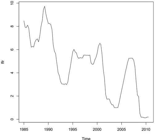
r∗t = πt+ δ(πt− π∗) + wˆyt+ R∗
where the r∗
t is the short-term nominal interest rate target, called Federal funds
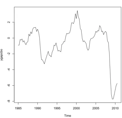
rate; the π∗ is about 2%, the ˆy
t is the deviation of output from its long-run
trend, called output gap. The R∗ is the equilibrium level of interest rate (real)
and it is about 2%.
3.1
The Model
The Households
The households consume and invest a quantity of retail goods and the utility function of the households is:
E��∞
t=0
βtAt(ln Ct− χNt)
�
(3.2)
where β ∈ (0, 1) is a parameter and is the subjective discount factor; At is the
3.1. THE MODEL 27
disutility from working and Nt is the fraction of household members who are
employed.
The growth rate of the intertemporal preference shocks is γat and it is the
ratio between Atand At−1. This growth rate follows the stochastic process1
ln γat= ρaln γa,t−1+ σatεat
where ρa∈ (−1, 1) is the persistence of preference shock, εatis a normal
indepen-dent iindepen-dentified distribution and σatdenotes the time-varying standard deviation
of innovation to preference shock and it is called preference uncertainty shock, which follows the stationary process:
ln σat= (1 − ρσa) ln σa+ ρσaln σa,t−1+ σσaεσa,t
where ρσa ∈ (−1, 1) measures the persistence of preference uncertainty; εσa,t is
the innovation to preference uncertainty shock and it is distributed as a normal
process; σσa is the constant standard deviation of the innovation.
The households maximize the utility function (3.2) subject to a budget con-straint, holds for all t:
Ct+ Bt PtRt = Bt−1 Pt + (1 − τt )[wtNt+ φ(1 − Nt)] + dt− Tt (3.3)
where Pt is the price level; Bt denotes the household’s holdings of nominal
risk-free bond; Rt denotes the nominal interest rate; wtdenotes the real wage
rate; φ denotes the unemployment benefit; dt denotes the profit income from
household’s ownership of intermediate goods producers and of retailers and Tt
is the lump-sum taxes.
We assume that τtis the labour income tax rate and it follows the stochastic
process:
ln τt= (1 − ρτ) ln τ + ρτln τt−1+ στ tετ t
where ρτ ∈ (−1, 1) is the persistence of tax shock; ετ t is an independent and
identically distributed (i.i.d.) normal process and στ t is the time-varying
stan-dard deviation of innovation to tax shocks and it is called the tax uncertainty
shock. The στ t follows the stationary process:
ln στ t= (1 − ρστ) ln στ+ ρστln στ,t−1+ σστεστ,t
where ρστ ∈ (−1, 1) measures the persistence of tax uncertainty, εστ,t is the
innovation to the tax uncertainty shock and is a standard normal process and
σστ is the (constant) standard deviation of the innovation.
The optimal bond-holding decisions result in the intertemporal Euler equa-tion: 1 = Etβγa,t+1 Λt+1 Λt Rt πt+1
where Λt denotes the marginal utility of consumption and πt = PPt−1t is the
inflation rate.
1A stochastic process is a family of random variables{xt: t∈ T } defined on a probability
28 CHAPTER 3. THE THEORETICAL MODEL The aggregation sector
The final consumption good, which is a basket of differentiated retail goods, is written as: Yt= �� 1 0 Yt(j) η−1 η � η η−1
where Yt(j) is a type j retail good for j ∈ [0, 1] and η > 1 denotes the elasticity
of substitution between differentiated products. We have the following problem:
min� 1
0
Pt(i)Yt(i)di s.t 1 = Yt
where Pt(j) is the price of retail good of type j and the demand for a type j
retail good is inversely related to the relative price:
Yd t(j) = �P t(j) Pt �−η Yt.
The price index Ptis related to the individual prices Pt(j) through the following
relation: Pt= �� 1 0 Pt(j) 1 1−η �1−η . The retail goods producers
We take a continuum of retail goods producer that produce a differentiated prod-uct using a homogenous intermediate good as input. The prodprod-uction function of retail good of type j ∈ [0, 1] is given by:
Yt(j) = Xt(j)
where Xt(j) is the input of intermediate goods used by retailer j and Yt(j) is
the output. The retail goods producers are price takers in the input market and monopolistic competitors in the product markets, where they set prices for their products. We assume that the price adjustment costs are in units of aggregate output and are subject to a quadratic cost
Ωp 2 � P t(j) πPt−1(j) − 1� 2 Yt
where the parameter Ωp ≥ 0 measures the cost of price adjustments and π
denotes the steady-state inflation rate.
A retail firm that produces good j solves the following profit-maximizing problem max Pt(j) Et ∞ � i=0 βiΛ t+i Λt �� Pt+i(j) Pt+i − q t+i � Yt+id (j) − Ωp 2 � Pt+i(j) πPt+i−1(j) −1 �2 Yt+i �
3.1. THE MODEL 29
where qt+idenotes the relative price of intermediate goods in period t + i. In a
symmetric equilibrium with Pt(j) = Pt for all j we have
qt= η− 1 η + Ωp η �π t π �π t π − 1 � − Et βΛt+1 Λt Yt+1 Yt πt+1 π �π t+1 π − 1 �� .
If Ωp = 0 (i.e. there is no price adjustment costs) the optimal pricing rule
implies that real marginal cost qt is the inverse of the steady state markup
(qt= (η − 1)/η).
The labor market
We assume that at the beginning of our analysis in period t there are ut
un-employed workers searching for jobs and there are vtvacancies posted by firms.
The matching variable is described using a Cobb-Douglas function2
mt= µuαtv1−αt
where mt is the number of successful matches and the parameter α ∈ (0, 1)
denotes the elasticity of job matches with respect to the number of searching workers and µ scales the matching efficiency.
We define two different rates related to the matching theory:
i) The job filling rate is the probability that an open vacancy is matched with
a searching workers, qv
t = mt/vt.
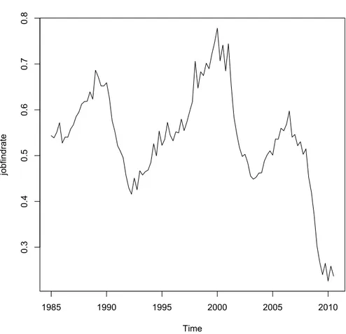
ii) The job finding rate is the probability that an unemployed and searching
worker is matched with an open vacancy, qu
t = mt/ut.
In period t there are Nt−1 workers, a fraction ρ of these workers lose their
jobs and we have that (1 − ρ)Nt−1 is the number of workers who survive the
job separation. At time t mtmatches are formed and we can assume that new
hires start working in the period they are hired, so we have that aggregate unemployment in period t evolves according to
Nt= (1 − ρ)Nt−1+ mt.
The number of unemployed workers searching for jobs in period t is
ut= 1 − (1 − ρ)Nt−1.
We assume full participation, i.e. at all times all individuals are either employed or willing to work and we have that the unemployment rate is:
Ut= ut− mt= 1 − Nt
and means the fraction of the population who are left without a job after hiring takes place in period t.
2The Cobb-Douglas function has the following form F (K, AL) = BKα(AL)1−αwhere the
parameters α∈ (0, 1) and B is assumed positive, the K,AL are variables that in the growth theory describe the capital and the effective labor force.
30 CHAPTER 3. THE THEORETICAL MODEL The firms (intermediate goods producers)
We know that a firm can produce a good only if a match with a worker is formed. The production function for a firm with one worker is
xt= Zt
where xt is the output and Zt is an aggregate technology shock, which follows
the stochastic process
ln Zt= (1 − ρz) ln Z + ρzln Zt−1+ σztεzt.
The ρz∈ (−1, 1) measures the persistence of the technology shock. The term εzt
is an i.i.d innovation to the technology shock and is a standard normal process.
The term σztis a time-varying standard deviation of the innovation, denotes the
technology uncertainty shock and it follows the stationary stochastic process
ln σzt= (1 − ρσz) ln σz+ ρσzln σz,t−1+ σσzεσz,t.
The parameter ρσz ∈ (−1, 1) measures the persistence of the technology
un-certainty, the εσz,t is the innovation to the technology uncertainty and is a
standard normal process and the parameter σσz > 0 is the standard deviation
of the innovation.
If a match is formed, the firms obtain a flow profit in the current period after paying the worker. In the t + 1 period, if the match survives (with probability 1 − ρ), the firm continues, otherwise (with probability ρ) the firm posts a new
job vacancy at a fixed cost κ with the value Vt+1. The value of a firm with a
match is therefore given by the Bellman equation
JtF = qtZt− wt+ Et βΛt+1 Λt � (1 − ρ)JF t+1+ ρVt+1 � . (3.4)
Each new vacancy posted in period t costs κ units of final goods, the vacancy
can be filled with probability qv
t and the firms obtain the value of the match.
Otherwise the vacancy remains unfilled and the firms go into the next period
with the value Vt+1, so we have that the value of an open vacancy is:
Vt= −κ + qvtJtF+ Et
βΛt+1
Λt (1 − q
v t)Vt+1.
Free entry implies that Vt= Vt+1= 0 and
κ = qvtJtF. (3.5)
If we put the equation (3.5) in the equation (3.4) we obtain: κ qv t = qtZt− wt+ Et βΛt+1 Λt (1 − ρ) κ qv t+1 . (3.6)
3.1. THE MODEL 31 Workers’ value function
If a worker is employed, he obtains an after-tax wage income and suffers a utility cost for working in period t. In the next period, the match is dissolved with probability ρ and the separated worker can find a new match with probability
qu
t+1. Otherwise the worker does not find a new job in t + 1 period with
proba-bility ρ(1 − qu
t+1) and so he enters in the unemployment pool. The (marginal)
value of an employed worker satisfies the Bellman equation:
JtW = (1−τt)wt− χ Λt +Et βΛt+1 Λt � [1−ρ(1−qu t+1)]Jt+1W +ρ(1−qut+1)Jt+1U � (3.7) where JU
t is the value of an unemployed household member. If a worker is
currently unemployed, then he obtains an after-tax unemployment benefit and
can find a new job in period t + 1 with probability qu
t+1. Otherwise he remains
unemployed. The value of an unemployed worker thus satisfies the Bellman equation is JtU = φ(1 − τt) + Et βΛt+1 Λt � qut+1Jt+1W + (1 − qt+1u )Jt+1U � . (3.8)
The Nash bargaining wage
The firms and the workers bargain over wages and we have the following Nash bargaining problem:
max
wt
(JW
t − JtU)b(JtF)1−b
where b ∈ (0, 1) is the bargaining weight for workers. We can define the total
surplus as St = JtF + JtW − JtU and the bargaining solution is given using the
first order condition and the total surplus equation:
JF
t = (1 − b)St JtW − JtU = bSt. (3.9)
Then from equations (3.7) and (3.8) we have that the total surplus is a function of the total surplus at time t + 1
bSt= (1 − τt)(wNt − φ) − χ Λt + EtβΛt+1 Λt � (1 − ρ)(1 − qu t+1)bSt+1 � . (3.10)
Using the equations (3.5),(3.9) and (3.10) we have the Nash bargaining wage3:
wNt [1 − τt(1 − b)] = (1 − b) � χ Λt+ φ(1 − τ t) � + b � qtZt+ β(1 − ρ)EtβΛt+1 Λt κvt+1 ut+1 � . The Nash bargaining wage is a weighted average of the worker’s reservation value and the firm’s productive value of a job match adjusted for labor income taxes borne by the worker. By forming a match, the worker incurs a utility cost of working and foregoes the after-tax unemployment benefit; the firm receives the marginal product from labor in the current period and saves the vacancy cost from the next period.
32 CHAPTER 3. THE THEORETICAL MODEL Government policy
The government finances exogenous spending Gt and unemployment benefit
payments φ through labor income taxes and lump-sum taxes. We assume that: i) the government balances the budget in each period so that
Gt+ φ(1 − Nt) = Tt+ τt[wtNt+ φ(1 − Nt)]
ii) the ration of government spending to output gt= Gt/Ytfollows the
station-ary stochastic process:
ln gt= (1 − ρg) ln g + ρgln gt−1+ σgεgt
where ρg ∈ (−1, 1) is the persistence parameter, the innovation εgt is
an i.i.d standard normal process, and σg is the time-varying standard
deviation of the innovation and it is an uncertainty shock to government spending.
The government spending uncertainty shock follows the stationary stochastic process
ln σgt= (1 − ρσg) ln σg+ ρσgln σg,t−1+ σσgεσg,t
where the parameter ρσg ∈ (−1, 1) is the persistence of uncertainty shock to
government spending, the term εσg,t denotes the innovation to the uncertainty
shock and is a standard normal process and the parameter σσg > 0 is the
standard deviation of the innovation.
The government conducts a monetary policy by following the Taylor Rule
Rt= rπ∗ �π t π∗ �φπ� Yt Y �φy
where the parameters φπ and φy determine respectively the aggressiveness of
monetary policy against deviations of inflation from the target π∗and the extent
to which monetary policy accommodates output fluctuations. The parameter r is the steady-state real interest rate and is equal R/π.
Search equilibrium
In a search equilibrium, the markets for bonds, capital, final consumption goods, and intermediate goods all clear.
Since the aggregate supply of the nominal bond is zero, the bond market-clearing condition implies that
Bt= 0.
The goods market clearing condition, that is Y = Cd+ Id+ G where Y is the
current production function, the Cdis the current demand for consumption; Id
is the demand for investment and G is government spending, implies:
Ct+ κvt+ Ωp 2 � πt π − 1 �2 Yt+ Gt= Yt.
3.1. THE MODEL 33
where Ytis the aggregate output of final goods.
The intermediate goods market clearing implies that:
Chapter 4
Data Analysis
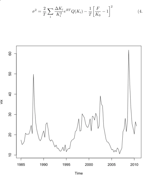
In this chapter we examine the theoretical model using actual data and we analyze the US quarterly data from the first quarter in 1985 to the third quarter in 2010. The data are: VIX Index, Economic Policy Uncertainty Index (created by Baker, Bloom and Davis), unemployment rate, quarterly inflation rate, job creation rate, job destruction rate, job-finding rate, Federal Funds rate and CBO’s output gap.
In the first part of this chapter we make a description of all these data. Then we create two different models and we estimate using a VAR model and we search the possible relationships between the policy uncertainty shock and the data related to the labor market (unemployment rate, job creation rate, job destruction rate and job-finding rate) and to the inflation.
In the second part we delete the data related to the 2008 financial crisis and search for possible differences between the two models. Finally we introduce a new variable, the new economic policy uncertainty index, created in 2013 and we focus on possible differences.
4.1
Data Description
VIX Index
The VIX index is the CBOE1 volatility index, which shows the market’s
ex-pectation of 30-day volatility. The VIX is based on the S&P 500 Index (SPX)2,
the core index for US equities, and estimates expected volatility by averaging the weighted prices of SPX puts and calls over a wide range of strike prices.
VIX is a volatility index comprised of options rather than stocks, with the price of each option reflecting the market’s expectation of future volatility. The
1Chicago Board Options Exchange is the world’s largest options exchange and it focuses
on options contracts for individual equities, indexes and interest rates.
2The Standard & Poor’s 500 Index (S&P 500) is a stock market index based on market
capitalizations of 500 leading companies publicly traded in the U.S. stock market.
36 CHAPTER 4. DATA ANALYSIS generalized formula for VIX index calculation is:
σ2= 2 T � i ∆Ki K2 i eRTQ(K i) − 1 T � F K0 − 1 �2 (4.1) Time vi x 1985 1990 1995 2000 2005 2010 10 20 30 40 50 60
Figure 4.1: VIX Index (1985:01-2010:03)
where σ is VIX/100 and VIX = σ ×100; T is the time to expiration; F is the
Forward index level3derived from the index option prices; K
0 is the first strike
below the forward index level; Kiis the strike price of the i-th out-of-the-money
option (if Ki > K0 it’s a call, otherwise it’s a put, if Ki = K0 it’s both a put
and a call); R is the risk-free interest rate to expiration and Q(Ki) represents
3To determine it, the CBOE chooses a pair of put and call options with prices that are
4.1. DATA DESCRIPTION 37
the average of the call and put option prices at strikes. Since K0 ≤ F , the
average at K0implies that CBOE uses one unit of the in-the-money call at K0.
The last term in the equation (4.1) represents the adjustment needed to convert this in-the-money call into an out-of-the-money put using put-call parity.
∆Ki is the interval between strike prices, it’s the difference between the
strike on either side of Ki: ∆Ki= (Ki+1− Ki−1)/2.
From the Figure 4.1, we see that there are some spikes in the 1987:04 and
1988:01 (Black Monday and stock market crash4.), also in the period between
2002 and 2004. In the period around 2008:04 and 2009:01, we have the biggest and strong increase and peak due to the financial crisis. Otherwise there are decreases in the period between 1992-1995 and 2005-2006 (where we have also the minimum in 2006) and in the mid of 2007. So an increase in the VIX index is related to the economic recession.
Economic Policy Uncertainty Index
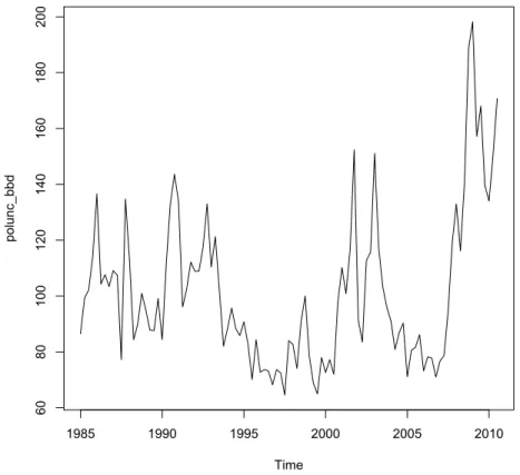
Baker, Bloom and Davis [2] construct the economic policy uncertainty in-dex using three types of underlying components. The first component quantifies the newspaper coverage of policy-related economic uncertainty, the second one uses the number of federal tax code provisions set to expire in future years and the third one utilizes disagreement among economic forecasters as a proxy of uncertainty.
a) News coverage is an index of search results from 10 U.S. newspapers: USA Today, the Miami Herald, the Chicago Tribune, the Washington Post, the Los Angeles Times, the Boston Globe, the San Francisco Chronicle, the Dallas Morning News, the New York Times and the Wall Street Journal. Baker, Bloom and Davis make month-by-month searches of each paper, starting in January 1985, for terms related to economic and policy uncer-tainty. They search in particular for articles containing the term ’uncer-tainty’ or ’uncertain’, the terms ’economic’ or ’economy’ and one or more of the following terms: ’policy’, ’tax’, ’spending’, ’regulation’, ’federal re-serve’, ’budget’, or ’deficit’. Then they count the number of articles that satisfy our search criteria each month, which create our monthly series. They normalize the raw counts by the number of news articles in the same newspapers that contain the term ’today’, and then calculate a backwards-looking 36-month moving average to smooth this series at a monthly level. For each newspaper they divide the policy-related uncertainty counts by the smoothed value of ’today’ series and they sum each paper’s series and normalize them to an average value of 100 from 1985 to 2010.
b) The tax code expiration is based on reports by the CBO5that makes lists of
temporary federal tax code provisions. The temporary tax code provisions
4See in Appendix A.1
5The CBO is the Congressional Budget Office, it produces independent analyses of
38 CHAPTER 4. DATA ANALYSIS lead to outlooks for federal spending and borrowing and to discrepancies
between the tax revenues projections of the CBO and OMB6. The CBO
uses ’current law’ as a baseline taking into account all scheduled tax ex-pirations, while the OMB uses ’current policy’ as a baseline under its assessment of which temporary provisions are likely to be extended. The CBO reports describe the tax code provisions and identifies the sched-uled expiration month and then they weight these data in January of each
year multiplying expirations by 0.5((T +1)/12)for T equal to the number of
months in the future when the tax code provision expires. Then they sum the discounted number of tax code expirations to have an index value for each January.
c) The economic forecaster disagreement is based on the Federal Reserve Bank of Philadelphia’s Survey of Professional Forecasters. This survey is also called the Anxious Index, is a highly report on the prospects for the econ-omy of the United States. This index often goes up just before the reces-sions began and is a quarterly one, each quarter every forecaster receives a form in which to fill out values corresponding to previsions for variables in each of the next five quarters. They use it for three of the forecast
vari-ables, the consumer price index (CPI)7, purchase of goods and services by
state and local governments, and purchase of goods and services by the federal government. They look at the quarterly previsions for the next year and they choose it because they are directly influenced by monetary policy and fiscal policy actions.
To build the dispersion component, they take the interquartile range of each set of inflation rate forecasts in each quarter, then they use the raw in-terquartile range. For both federal and state/local government purchases, we divide the interquartile range of four-quarter-ahead forecasts by the median four-quarter-ahead forecast and multiply that quantity by a 5-year backward-looking moving average for the ratio of nominal purchases to nominal GDP. They sum the two weighted values to build up the single federal/state/local index and they look at the interquartile range scaled by the ratio of governments purchases to the economy.
To build up our index they normalize each component by its own stan-dard deviation and then they compute an average value of the components, using weights of 1/2 on news-index and 1/6 on each of the other three mea-sures (tax expirations index, the CPI forecast disagreement measure, and the federal/state/local purchases disagreement measure).
The policy uncertainty index can be calculated using other two weighting methodologies. First, they equally weight the news-based measure, the
combi-6The OMB is the Office of Management and Budget and it assists the U.S. President to
prepare the budget.
7The CPI is a measure of the average change over time in the prices paid by urban
con-sumers for a market basket of consumer good and services. It can be used as a measure of inflation and is viewed as an indicator of the effectiveness of government economic policy. It’s computed by the Bureau of Labor Statistics.
4.1. DATA DESCRIPTION 39 nation of the forecast disagreement measures, and the tax expiration measure. Second, they perform a principle component analysis on four previously series to obtain weights for each components and the weights are: 0.35 on news-based index. 0.37 on tax expirations index, 0.24 on the CPI forecast disagreement measure, and 0.04 on our federal expenditure disagreement measure.
From the figure 4.2 we find spikes related to Lehman Brother’s bankruptcy
and TARP8 and banking crisis and Obama election in 2008-2009. We can see
also a spike at the end of 2001, due to the 9/11, and a spike in the 2003, due to the Second Gulf War. In the plot we can also see a spike at the beginning of 1987 (the Black Monday) and in 1990 (the First Gulf War).
Time po lu nc_ bb d 1985 1990 1995 2000 2005 2010 60 80 100 120 140 160 180 200
Figure 4.2: Policy-Related Economic Uncertainty Index (1985:01-2010:03)
8The Troubled Asset Relief Program(TARP) is created to implement programs to stabilize
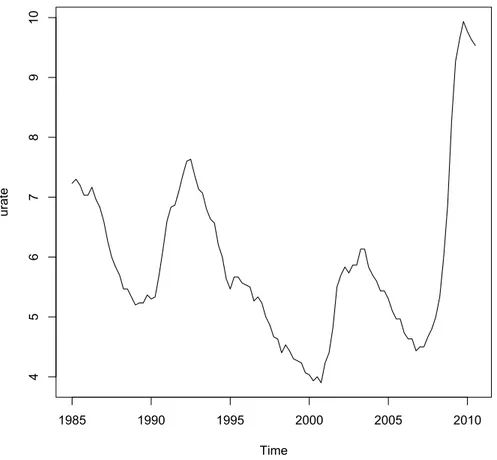
40 CHAPTER 4. DATA ANALYSIS Unemployment Rate
The unemployment rate is calculated by the Bureau of Labor Statistics (BLS) of the U.S. Department of Labor and it’s the percent of the labor force that is unemployed. Persons are classified as unemployed if they do not have a job, have actively looked for a work in the prior 4 weeks, and are currently available for work.
Actively looking for a work may consist of: having a job interview, sending out resumes or filling out applications, placing or answering advertisements, etc. The research is based on questions related to work and searching jobs and it is based on the civilian noninstitutional population 16 years old and over.
Time ura te 1985 1990 1995 2000 2005 2010 4 5 6 7 8 9 10
Figure 4.3: Unemployment Rate (1985:01-2010:03)
From the figure 4.3 we can see that we have high spikes from 2009 till our days, the unemployment rate grows up till 9.7% and this increase is due to the