ALMA MATER STUDIORUM - UNIVERSITÀ DI BOLOGNA
SCUOLA DI INGEGNERIA E ARCHITETTURA
DIPARTIMENTO DEI
CORSO DI LAUREA in AUTOMATION ENGINEERING
TESI DI LAUREA
in
Industrial Robotics
Condition Monitoring of a Belt-Based Transmission System
for Comau Racer3 Robots
CANDIDATO RELATORE:
Chiar.mo Prof. Claudio Melchiorri Roberta Tanzariello
CORRELATORE/CORRELATORI Ing. Marco Robusti
Anno Accademico 2016/2017
iii
iv
Condition Monitoring of a Belt-Based
Transmission System for Comau
v
In fin dei conti, non temete i momenti difficili.
Il meglio scaturisce da lì. Rita Levi Montalcini
iii
A
CKNOWLEDGEMENTS
I ackowledge and thank my Advisor Claudio Melchiorri for the opportunity given through the AlmaTong Project, my Co-Advisor Marco Robusti and the all team PD Cost Engineering of Comau Kunshan for all the advise, insight and discussion over my intership that has led to the completion of the work.
Special Thanks to Aldo Maria Bottero, Gagliano Alberto and the Performance Engineering Team for their knowledge shared and the support provided in the high frequency acquisition. I would like to thank all the PD department of Comau Italy for the assistance and conversation about the development of the test plan. Additional thanks to Zhou Shaohua for the support in the installation of the FTP connection, Kuai Peng Loki and Cheng Yu for the simulation of the fault. Special thanks to Davide Miceli, Luca Menzio and the all team of Innovation Specialists for the collaboration and the support given in the implementation of the Automatic Acquisition.
iv
A
BSTRACT
This project has been developed in collaboration with Comau Robotics S.p.a and the main goal is the development in China of an Health Monitoring Process using vibration analysis. This project is connected to the activity of Cost Reduction car-ried out by the PD Cost Engineering Department in China.
The Project is divided in two part:
1. Data Acquisition 2. Data Analysis
An Automatic Acquisition of the moni.log file is carried out and is discussed in Chapter 1. As for the Data Analysis is concerned a data driven approach is con-sidered and developed in frequency domain through the FFT transform and in time domain using the Wavelet transform.
In Chapter 2 a list of the techiques used nowadays for the Signal Analysis and the Vibration Monitoring is shown in time domain, frequency domain and time-frequency domain.
In Chapter 3 the state of art of the Condition Monitoring of all the possible machi-nery part is carried out from the evaluation of the spectrum of the current and speed.
In Chapter 4 are evaluated disturbances that are not related to a fault but belong to a normal behaviour of the system acting on the measured forces. Motor Torque Ripple and Output Noise Resolution are disturbance dependent on velocity and are mentioned in comparison to the one related to the configuration of the Robot. In Chapter 5 a particular study case is assigned: the noise problem due to belt-based power transmission system of the axis three of a Racer 3 Robot in Endu-rance test. The chapter presents the test plan done including all the simulations. In Chapter 6 all the results are shown demostrating how the vibration analysis carried out from an external sensor can be confirmed looking at the spectral con-tent of the speed and the current.
In the last Chapter the final conclusions and a possible development of this thesis are presented considering both a a Model of Signal and a Model Based approach.
v
Questo progetto è stato sviluppato in collaborazione di Comau S.p.A e l’obiettivo è lo sviluppo di un “Health Monitoring Process” usando l’analisi vibrazionale è inoltre connesso all’attività di riduzione dei costi portata avanti in Cina dal PD Cost Engineering Department .
Il progetto è diviso in due parti: 1. Acquisizione dei dati 2. Analisi dei dati
L’Acquisizione Automatica del file moni.log è discussa nel Capitolo 1. Un ap-proccio di tipo data driven è stato usato per l’analisi dei dati e sviluppato nel do-minio della frequenza secondo trasformata FFT e in dodo-minio tempo frequenza usando la trasformata Wavelet.
Nel Capitolo 2 è riportato un elenco di tutte le tecniche usate oggi per l’analisi del segnale e il monitoraggio delle vibrazioni nel dominio del tempo, della frequenza o tempo frequenza.
Nel Capitolo 3 lo stato dell’arte riguardo il monitoraggio di componenti meccanici è sviluppato dall’analisi dello spettro di corrente e velocità.
Nel Capitolo 4 sono considerati disturbi non connessi a guasti ma appartenenti al comportamento nominale del sistema e che agiscono sulle Forze. “Motor Tor-que Ripple” e “Output Noise Resolution” sono disturbi che dipendono dalla velo-cità al contrario di quelli che dipendono dalla configurazione del Robot.
Nel Capitolo 5 è stato assegnato e sviluppato il problema di un rumore nella tra-smissione dell’asse tre del Robot Racer 3 in Endurance Test. Il Capitolo riporta il progetto dei test condotti e le rispettive simulazioni.
Nel Calitolo 6 sono riportati e commentati tutti i risultati con l’intento di dimostrare come l’analisi della vibrazione fatta da un sensore esterno può essere confermata dallo spettro di corrente e velocità.
Nell’ultimo capitolo sono riportati le conclusioni finali e i possibili sviluppi della tesi basati sul Modello e sul Modello del segnale.
vi
L
IST OF
F
IGURE
Figure 1.1 Timings of action for maintenance ... 1
Figure 1.2 An integrated approach to CBM/PHM design... 3
Figure 1.3 CBM/PHM online and offline phase ... 3
Figure 1.4 Part of the DFMEA considered in the project ... 4
Figure 1.4 Not Automatic Acquisition for the Collection of Moni.log... 5
Figure 1.5 Map of the cells connected ... 6
Figure 1.6 Racer Family Robots ... 6
Figure 1.7 WinC5G interface ... 7
Figure 1.8 Automatic Acquisition performed ... 7
Figure 1.9 Features displayed during the Automatic Acquisition ... 8
Figure 2.1 Skewness, a measure of the symmetry of a distribution ... 11
Figure 2.2 The Kurtosis, a measure of the size of the side lobes of a distribution ... 12
Figure 2.3 Matrix representation of the DFT (note the rotating and imaginary part) ... 14
Figure 2.4 Signal schematic classification ... 15
Figure 2.5 Time-frequency resolution of: (a) Short-Time-Fourier-Transform (STFT) and (b) Wavelet Transform (WT) ... 17
Figure 2.6 Mother Wavelet with (a) large scale and (b) small scale ... 19
Figure 2.7 Subband Algorithm ... 21
Figure 2.8 The Haar Wavelet ... 23
Figure 3.1 FFT analysis-unbalanace ... 27
Figure 3.2 Phase relationship-static unbalance ... 27
Figure 3.3 Phase relationship-couple unbalance ... 28
Figure 3.4 A belt driven fan/blower with an overhung rotor – the phase is measured in the axial direction ... 28
Figure 3.5 A belt-driven fan/blower – vibration ... 29
Figure 3.6 Eccentric rotor ... 29
Figure 3.7 An FFT of a bent shaft with bend near the shaft center ... 30
Figure 3.8 Note the 180 ° phase different in the axial direction ... 30
Figure 3.9 Angular misalignment ... 32
Figure 3.10 FFT of angular misalignment ... 32
Figure 3.11 Angular misalignment confirmed by phase analysis ... 33
Figure 3.12 Parallel misalignment ... 33
Figure 3.13 FFT of parallel misalignment ... 34
Figure 3.14 Radial phase shift of 180° is observed across the coupling ... 34
Figure 3.15 loose internal assembly graph ... 35
Figure 3.16 Loose fit ... 35
Figure 3.17 Mechanical looseness graph ... 36
Figure 3.18 Mechanical looseness ... 36
Figure 3.19 Structure looseness ... 37
Figure 3.20 Structure looseness graph ... 37
Figure 3.21 Characteristic frequencies of the bearing of axis 3 ... 39
Figure 3.22 Small defect in the raceways of a bearing ... 40
Figure 3.23 More obvious wear in the form of pits ... 40
Figure 3.24 Wear is now clearly visible over the breath of the bearing ... 41
Figure 3.25 Severely damaged bearing in final stage of wear ... 41
vii
Figure 3.27 Gear tooth wear ... 43
Figure 3.28 Gear tooth load ... 43
Figure 3.29 Gear eccentricity and backlash ... 44
Figure 3.30 Gear Misalignment ... 45
Figure 3.31 Gears-cracked ... 45
Figure 3.31 Sub-harmonic belt frequencies ... 46
Figure 3.32 Misalignment types (the pigon toe and angle are classified as angular misalignment)... 47
Figure 3.33 Vibration due to sheave misalignment ... 47
Figure 3.34 Vibration due to sheave misalignment ... 48
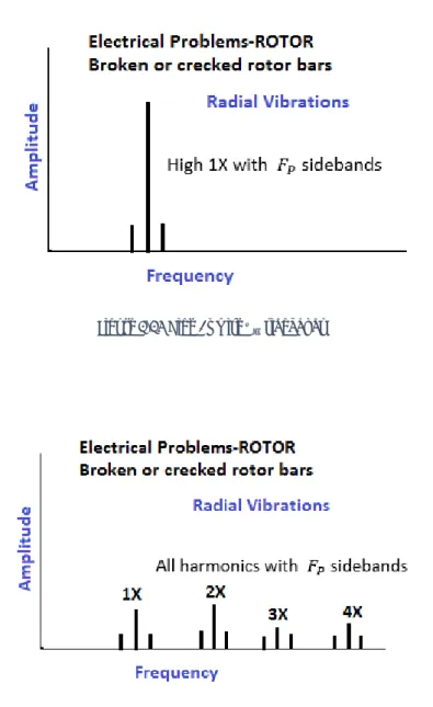
Figure 3.35 High 1x with 𝐹𝑃 sidebands... 50
Figure 3.36 All harmonics with 𝐹𝑃 sidebands ... 50
Figure 3.37 Rotor bar pass frequency ... 51
Figure 3.38 Eccentric Rotor ... 52
Figure 3.39 Stator defects ... 52
Figure 3.40 Synchronous motors ... 53
Figure 4.1 Dependence of the torque ripple on the angular position and current ... 58
Figure 4.2a Speed response to the torque disturbance ... 60
Figure 4.2b Control Scheme ... 60
Figure 4.3 TRC effect on ax 3 of a NJ 420-3.0 manipulator ... 61
Figure 4.4 Load Accelerator with TRC not active and active on a NJ4 175-2.5 manipulator ... 62
Figure 4.5 Basic adaptive copensator for sinusoidal disturbances ... 63
Figure 4.6 Feed forward disturbance compensation ... 64
Figure 4.7 The complete architecture of the adaptive compensator ... 64
Figure 5.1 Vibration power of the signal coming from the sensor ... 69
Figure 5.2 Vibration power versus velocity ... 69
Figure 6.1: Experimental test bed for displacement sensor ... 70
Figure 6.2: Experimental test bed for Accelerometer ... 71
Figure 6.3: CMOS type Micro Laser Distance Sensor HG-C ... 72
Figure 6.4: The interface TracerDAQ Pro ... 72
Figure 6.5.a and Figure 6.5.b: Position of the accelerometer in case of Axial and Radial vibration respectively ... 73
Figure 6.6: Axial vibration in term of voltage in nominal case 25% of the maximum speed ... 73
Figure 6.7: Axial vibration in Matlab environment 25% of the maximum speed ... 74
Figure 6.8: Belt-Transmission Based transmission ... 75
Figure 6.9 Angular Misalignment ... 76
Figure 6.10 Addiction of Spacers for the simulation of the Angular Misalignment ... 76
Figure 6.11 FFT in case of Angular Misalignment ... 76
Figure 6.12 Parallel Misalignment ... 77
Figure 6.13 FFT in case of Parallel Misalignment ... 77
Figure 6.14 LImitations in space considered for the simulation of the fault Unbalance ... 78
Figure 6.15 FFT of the fault Unbalance ... 79
Figure 6.16 Simulation of Loseness ... 79
Figure 6.17 FFT in case of Loseness ... 80
Figure 6.19. Damaged Belt ... 80
Figure 6.20 Application of a Damaged Belt ... 80
Figure 6.21 Transversal Vibration in Nominal case ... 81
Figure 6.22 Transversal Vibration in case of fault ... 82
viii
Figure 6.24 Time interval with Constant Velocity ... 82
Figure 6.25 Trace of the entire vibration obtained at constant velocity ... 83
Figure 6.26 Points from which the vibration is recorded ... 83
Figure 6.26 Delta of the entire vibration obtained at constant velocity... 84
Figure 6.27 Delta of the first vibration obtained at constant velocity ... 85
Figure 6.28 Delta of the second vibration obtained at constant velocity ... 85
Figure 6.29 Haar 8 level wavelet transform used for the temporal analysis ... 86
Figure 6.30 Interval of time between vibration confirmed... 86
Figure 6.31 Mass added for the simulation of Unbalance ... 87
Figure 6.32 FFT in case of Unbalance ... 87
Figure 6.32 Comparison in the spectrum of the speed with 5% of the maximum speed... 88
Figure 6.33 Comparison in the spectrum of the speed with 75% of the maximum speed... 88
Figure 6.34 Comparison in the spectrum of the voltage with 5% of the maximum speed ... 89
Figure 6.35 FFT in case of Internal Assembly Loseness ... 89
Figure 6.36 FFT of the voltage in case of Internal Assembly Loseness at 25% of the maximim speed: different rate are considered ... 90
Figure 6.37 FFT of the speed in case of Internal Assembly Loseness at 25% of the maximim speed ... 90
ix
L
IST OF
T
ABLES
Table 1 Domain selection for diagnostic information ... 25
Table 2 Frequencies of the belt at different speed of the motor ... 66
Table 3 Frequencies of the Driver and Driven Pulley at different speed of the motor ... 66
Table 4 Inertia of the different components ... 68
x
C
ONTENTS
Acknowledgements ... iii Abstract ... iv List of Figure ... vi List of Tables ... ix1 Introduction to Structural Health Monitoring and Condition Based Monitoring ... 1
1.1 Introduction ... 1
1.2 Structural Health Monitoring Process ... 2
1.3 Scope of the Project ... 4
2 Vibration Monitoring and Signature Analysis ... 9
2.1 Signal Processing in Time domain ... 9
2.2 Signal Processing in Frequency domain ... 13
2.3 Signal Processing in Time-Frequency domain ... 14
2.3.1 Non-stationary signal processing ... 15
3 Condition Based Monitoring of Rotating Machine using Vibration Analysis ... 24
3.1 Introduction ... 24 3.2 Unbalance ... 25 3.3 Eccentric rotor ... 28 3.4 Bent Shaft ... 29 3.5 Misalignment... 30 3.5.1 Angular misalignment ... 31 3.5.2 Parallel misalignment ... 33 3.6 Mechanical looseness ... 34
3.6.1 Internal assembly looseness ... 34
3.6.2 Looseness between machine to base plate ... 35
3.6.3 Structure looseness ... 36
3.7 Rolling element Bearing ... 37
3.8 Gearing defects ... 41
3.9 Belt defects ... 45
3.10 Electrical Problems ... 48
3.10.1 Rotor problems ... 49
4 Condition Based Monitoring of Disturbance acting on the measured Force ... 54
4.1 Velocity independent disturbance ... 54
xi
4.2.1 Resolver output noise ... 56
4.2.2 Motor torque ripple ... 57
5 Case Study: Abnormal noise on Axis 3 due to a belt-based Power Transmission System 66 5.1 Belt Based Power transmission ... 66
5.1.1 Frequency Analysis ... 66
5.1.2 Temporal Analysis ... 68
6 Experimental Results ... 70
6.1 Experimental Set Up ... 70
6.1.1 High frequency acquisition from a signal controller ... 71
6.1.2 Acquisition from a displacement sensor ... 71
6.1.3 Acquisition from an accelerometer ... 73
6.2 Test Plan ... 74
6.2.1 NOMINAL CASE ... 75
6.2.2 ANGULAR MISALIGNMENT ... 75
6.2.3 PARALLEL MISALIGNMENT ... 77
6.2.4 EXCESSIVE LOAD UNBALANCE ... 78
6.2.5 INTERNAL ASSEMBLY LOSENESS ... 79
6.2.6 TOOTH SHEAR... 80
6.3 Testing Result ... 81
6.3.1 Tooth shear ... 81
6.3.2 UNBALANCE ... 86
6.3.3 INTERNAL ASSEMBLY LOSENESS ... 89
7 Conclusions and Future Work ... 91
7.1 Conclusions ... 91
7.2 Future Work ... 91
References ... 93
1
1 I
NTRODUCTION TO
S
TRUCTURAL
H
EALTH
M
ONITORING
AND
C
ONDITION
B
ASED
M
ONITORING
1.1
I
NTRODUCTIONMaintenance is a combination of science, art, and philosophy. The rationalization of maintenance requires a deep insight into what maintenance really is. Efficient maintenance is a matter of having the right resources in the right place at the right time. Maintenance can be defined as the total activities carried out in order to restore or renew an item to working condition, if fault is there. Maintenance is also defined as combination of action carried out to return an item to or restore it to an acceptable condition. The classification of maintenance according to timings of action for maintenance is shown in Figure 1.
______________________________________________________________________
Timing of Action Maintenance Operating to failure Shutdown or breakdown Fixed time based Preventive
Condition based Predictive or Diagnostic
Figure 1.1 Timings of action for maintenance
Every machine component behaves as an individual. Failure can take place ear-lier or later than recommended in case of preventive maintenance. It can be im-proved by condition based maintenance. Condition-based maintenance is defi-ned as “maintenance work initiated as a result of knowledge of the condition of an item from routine or continuous checking.” It is carried out in response to a significant deterioration in a unit as indicated by a change in a monitored para-meter of the unit condition or performance. Condition reports arise from human observations, checks, and tests, or from fixed instrumentation or alarm systems grouped under the name condition monitoring. It is here that one can make use of predictive maintenance by using a technique called signature analysis. Si-gnature analysis technique is intended to continually monitor the health of the
2
equipment by recording systematic signals or information derived from the form of mechanical vibrations, noise signals, acoustic and thermal emissions, change in chemical compositions, smell, pressure, relative displacement, and so on. Condition-based maintenance differs from both failure maintenance and fixed-time replacement. It requires monitoring of some condition-indicating parameter of the unit being maintained. This contrasts with failure maintenance, which im-plies that no successful condition monitoring is undertaken and with fixed-time replacement which is based on statistical failure data for a type of unit. In general, condition based maintenance is more efficient and adaptable than either of the other maintenance actions. On indication of deterioration, that unit can be sche-duled for shutdown at a time chosen in advance of failure, yet, if the production policy dictates, the unit can be run to failure. Alternatively, the amount of unne-cessary preventive replacement can be reduced, while if the consequences of failure are sufficiently dire, the condition monitoring can be employed to indicate possible impending failure well before it becomes a significant probability.
The trend monitoring method for one or group of similar machines is possible if sufficient data of monitored parameters are available. It relates the condition of machine(s) directly to the monitored parameters. On the other hand, condition checking method is employed for a wide range of diagnostics instruments apart fromhuman senses. Some of the recent developments in the form of CBM are proactive maintenance, reliability centered maintenance (RCM) and total produc-tive maintenance (TPM).
1.2 S
TRUCTURALH
EALTHM
ONITORINGP
ROCESSPrognostic and health management refers specifically to the phase involved with predicting future behaviour, including remaining useful life (RUL), in terms of cur-rent operating state and the scheduling of required maintenance action to man-tain system health. Detecting a component fault or incipient failure for a critical dynamic system and predicting its remaining useful life necessitate a series of studies that are intended to familiarize the CBM/PHM designer with the phisics of the failure mechanisms associated with the particular system/component. Failure modes and affects criticality analysis (FMECA) forms the fundation for a good
3
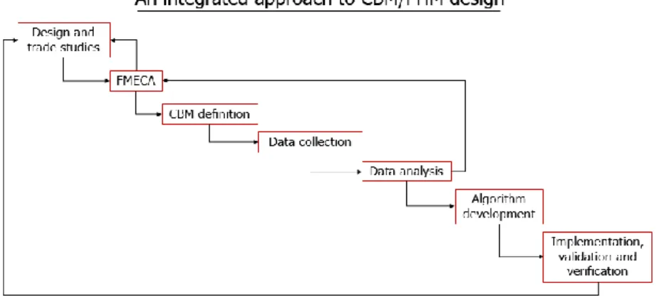
CBM/PHM design. A FMECA study decides the severity of candidate failure mode, their frequency of occurrence and their testability. In fig. 1.2 the main mo-dules of an integrated approach to CBM/PHM system design with the system-based components of the architecture: the feedback loops are intended to opti-mize the approach and complete the data collection and analysis steps that are essential inputs to the development of the fault diagnostic and prognostic algo-rithm.
Figure 1.2 An integrated approach to CBM/PHM design
In Figure 1.3 is possible to identify a preliminary offline phase and an online phase of CBM/PHM. The online phase inclused obtaining machinery data from sensors, signal preprocessing, extracting the features that are the most useful for determi-ning the current status or fault condition of the machinery, fault detection and classification, prediction of fault evolution and scheduling of required mainte-nance.
4
The offline phase consists of the required background studies that mus be per-formed offline prior to implementation of the online CBM phase and include de-termination of wich features are the most important for machine condition assess-ment, the FMECA, the collection of machine legacy fault data to allow useful pre-diction of fault evolution, and the specification of available personnel resources to perform maintenance actions.
Failure mode and effect analysis (FMEA)
Understanding the phisics of failure mechanisms constitute the cornerstone of good CBM/PHM system design. FMECA study attempts to relate failure events to their root causes. Towards this goal it addresses issues of identifying failure modes, their severity, frequency of occurrence, and testability; fault symptoms that are suggestive of the system’s behavior under fault conditions; and the sen-sors/monitoring apparatus required to monitor and track the system’s fault-symp-tomatic behaviors.
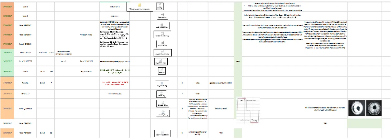
In this project the DFMEA of the trasmission of axis 3 of the Racer 3 is taken under consideration for the development of the test plan described in Chapter 5. In Fig. 1.4 only a part of the file is visible.
Figure 1.4 Part of the DFMEA considered in the project
1.3
S
COPE OF THEP
ROJECTThe activity carried out during my internship in Comau Robotics Kunshan starts from the construction of an automatic system of acquisition as already done in Italy in order to perform a systematic monitoring of the robots.
5
The file to be acquired automatically is called moni.log and contains inside all the information regarding current, velocity and acceleration for each joint of the ma-nipulator.
In order to understand the common faults or alarm for each robot I started my activity recording all the fault with the lastmoni.log associated in an excel file. All the other information are also specified (Date, Type of test, Cycle number/ Time, Observed data, Type of failure, Axis, Component, Observed effect, Occurrence, Future effect, Action taken). The lastmoni.log are taken manually by ethernet ca-ble.
Figure 1.4 Not Automatic Acquisition for the Collection of Moni.log
To start an automatic acquisition we set an FTP connection in order to make all the robots visible and controllable by remote first introducing Internet in all the cells and then setting properly the Subnet Mask and the Gateway from the Touch Pendant of the Robots. In the following picture is shown the map of all the cells connected divided according to the test going on: MFG-Manufactoring and Sign Off area. Endurance testing and Validation Testing for components.
6
Figure 1.5 Map of the cells connected
The Robots considered for the acquisition are the Racer Family (Racer 3, 5 and 5L) Racer Plus 7-1.4, 7-1.0 see Figure 1.6 and the Scara Robot (Rebel). The vibration analysis is performed instead on the Racer 3 robot in chapters 6.
Figure 1.6 Racer Family Robots
The WinC5G is the PC interface for the C5G Robot Controller. From the termi-nal is possible to see the actual status of the Robot. Is possible also to have the access to the program active the last moni.log, the history of the error and the alarm happened.
7
Figure 1.7 WinC5G interface
Without changing the standard run in program is possible to acquire automati-cally all the lastmoni.log from all the robots in the plant. The Software Moni Col-lector used is provided by Innovation Specialists in Comau Italy.
Figure 1.8 Automatic Acquisition performed
8
9
2 V
IBRATION
M
ONITORING AND
S
IGNATURE
A
NALYSIS
The word signature has been coined to designate signal patterns which charac-terize the state or condition of a system from which they are acquired. Signatures are extensively used as a diagnostic tool for mechanical system. In many cases, some kind of signal processing is undertaken on those signals in order to en-hance or extract specific features of such vibration signatures. It is very important to consider the type and range of transducers used as pickup for capturing vibra-tion signal. Signature-based diagnostic makes extensive use of signal processing techniques involving one or more methods to deal with the problem of improve-ment in the signal to noise ratio. Vibration-based monitoring techniques have been widely used for detection and diagnosis of bearing defects for several de-cades. These methods have traditionally been applied, separately in time and frequency domains. A time-domain analysis focuses principally on statistical cha-racteristics of vibration signal such as peak level, standard deviation, skewness, kurtosis, and crest factor. A frequency domain approach uses Fourier methods to transform the time-domain signal to the frequency domain, where further ana-lysis is carried out, using both the time and space domain according to the Multi-resolution Analysis.2.1 S
IGNALP
ROCESSING INT
IME DOMAINTo use information from CBM/PHM sensors for diagnosis, one must known how to compute statistical moments, which we describe in this section. The fourth mo-ment, kurtosis, has been found to be especially useful to capture the bang-bang types of motion owing to loose or broken components.
Given a random variable, its oth moment is computed using the ensemble ave-rage
𝐸(𝑥𝑃) = ∫ 𝑥𝑃𝑓(𝑥)𝑑𝑥
With 𝑓(𝑥) the probability density function (PDF). If a random variable is ergodic,
10
Moments about Zero and Energy
Given a discrete time series 𝑥𝑘, the pth moment over the time interval [1, N] is
given by 1 𝑁∑ 𝑥𝑘 𝑝 𝑁 𝑘=1
The first moment is the (sample) mean value
𝑥̅ = 1 𝑁∑ 𝑥𝑘
𝑁
𝑘=1
And the second moment is the moment of the inertia
1 𝑁∑ 𝑥𝑘
2 𝑁
𝑘=1
As N become larger, these better approximate the corresponding esemple ave-rages. The energy of the time series over the time interval [1, N] is given by
∑ 𝑥𝑘2 𝑁
𝑘=1
And the root mean square value (RMS) is
√1 𝑁∑ 𝑥𝑘
2 𝑁
𝑘=1
Moments about the Mean.
Given a time series 𝑥𝑘, the pth moment about the mean over the time interval
[1, N] is given by 1 𝑁∑(𝑥𝑘− 𝑥̅) 𝑃 𝑁 𝑘=1
11 𝜎2=1 2∑(𝑥𝑘− 𝑥̅) 2 𝑁 𝑘=1
Where σ is the standard deviation. Unfortunately, the sample variance is a biased estimate of the true ensemble variance, so in statistics one often uses instead the unbiased variance:
𝑠2= 1
𝑁 − 1∑(𝑥𝑘− 𝑥̅)
2 𝑁
𝑘=1
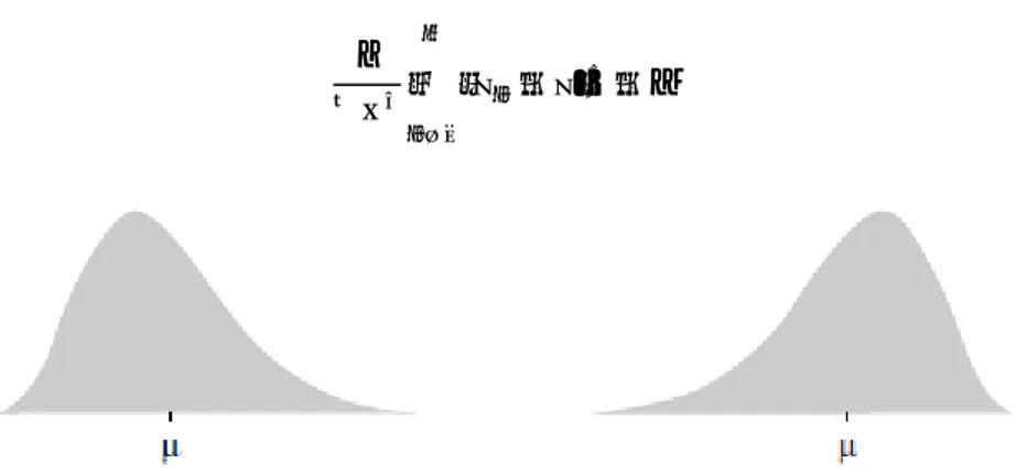
The third moment about the mean contains information about the simmetry of a distribution. A commonly used measure of simmetry is the skewness
1
𝑁𝜎3∑(𝑥𝑘− 𝑥̅)3 𝑁
𝑘=1
Skewness vanishes for simmetry distributions and is positive (negative) if the di-stribution develop along tail to the right (left) of the mean E(x). It measures the amount of spread of the distribution in either direction from the mean. Both pro-bability density functions (PDF) of Fig 2.1 have the same mean and standard deviation. The one on the left is posetively skewed. The one on the right is nega-tively skewed.
Also useful define the kurtosis, as
1
𝑁𝜎4∑(𝑥𝑘− 𝑥̅)4− 3 𝑁
𝑘=1
Figure 2.1 Skewness, a measure of the symmetry of a distribution
The kurtosis measures the contribution of the tails of the distribution, as illustra-ted in Fig. 2.2. The PDF on the right has higher kurtosis than the one on the left.
12
It is more peaked at the center, and it it has fatter tails. It is possible for a distri-bution to have the same mean, variance and skew amd not have the same kur-tosis measurement.
Correlation, Covariance, Convolution The (auto)correlation is given by
𝑅𝑥 =
1
𝑁∑ 𝑥𝑘𝑥𝑘+𝑛
𝑁
𝑘=1
Figure 2.2 The Kurtosis, a measure of the size of the side lobes of a distribution
Note that 𝑁𝑅𝑥(0) is the energy. The (auto)covariance is given as
𝑃𝑥(𝑛) = 1 𝑁∑(𝑥𝑘− 𝑥̅) 𝑁 𝑘=1 (𝑥𝑘+𝑛− 𝑥̅) Note that 𝑃𝑥(0) = 𝜎2.
Given two time series 𝑥𝑘 and 𝑦𝑘 the cross correlation is
𝑅𝑥𝑦(𝑛) = 1 𝑁∑ 𝑥𝑘 𝑁 𝑘=1 𝑦𝑘+𝑛
And the cross-covariance is
𝑃𝑥𝑦(𝑛) = 1 𝑁∑(𝑥𝑘− 𝑥̅) 𝑁 𝑘=1 (𝑦𝑘+𝑛− 𝑦̅)
13 𝑟 = ∑𝑥𝑘𝑦𝑘− ∑𝑥𝑘∑𝑦𝑘 𝑁 √[∑𝑥𝑘2−(∑𝑥𝑘 2) 𝑁 ] [∑𝑦𝑘2− (∑𝑦𝑘2) 𝑁 ]
The discrete time convolution for N point sequences is given as
𝑥 ∗ 𝑦(𝑛) = ∑ 𝑥𝑘𝑦𝑛−𝑘 𝑁−1
𝑘=0
Which is nothing more than polynimial multiplication. It is interesting to note that the correlation is expressed in terms of the convolution operator by
𝑅𝑥𝑦(𝑛) = 1 𝑁∑ 𝑥𝑘 𝑁 𝑘=1 𝑦𝑘+𝑛 = 1 𝑁 𝑥(𝑘) ∗ 𝑦(−𝑘)
2.2
S
IGNALP
ROCESSING INF
REQUENCY DOMAINDiscrete Furier Transform
The continuous infinite integrals of the Fourier transform become finite sums, usually expressed as 𝐺(𝑘) = (1 𝑁⁄ ) ∑ 𝑔(𝑛)exp (−𝑗2𝜋𝑘𝑛/𝑁) 𝑁−1 𝑛=0 𝑔(𝑛) = ∑ 𝐺(𝑘)exp (𝑗2𝜋𝑘𝑛/𝑁) 𝑁−1 𝑘=0
This version, known as the discrete Fourier transform (DFT), corresponds most closely to the Fourier series in that the forward transform is divided by the length of record N to give correctly scaled Fourier series components. If the DFT is used with other types of signals, for example transients or stationary random signals, the scaling must be adjusted accordingly as discussed below. The forward DFT operation can be understood as the matrix multiplication
𝐺𝑘 =
1
14
Figure 2.3 Matrix representation of the DFT (note the rotating and imaginary part)
Where 𝐺𝑘 represents the vector of N frequency components, the G(k), while 𝑔𝑘
represents the N time samples g(n). 𝑊𝑘𝑛 represents a square matrix of unit
vec-tors exp(-j2πkn/N) with angular orientation depending on the frequency index k (the rows) and time sample index n (the columns). This is illustrated graphically. For k=0 the zero frequency value G(0) is simply the mean value of the time sam-ples g(n) as would be expected. For k=1 the unit vector rotates -1/N th of a lution for each time sample increment resulting in one complete (negative) revo-lution after N samples. For higher values of k rotation speed is proportionally hi-gher. For k=N/2 (half the sampling frequency, the so called ‘Nyquist frequency’) the vector turns through -π for each time sample, but it is not possible to see in which direction it has turned. For k>N/2 the vector turns through less than π (in the negative direction) but is more easily interpreted as having turned through less than π (in the opposite direction) and thus if the time signal has been low pass filtered at half the sampling frequency (as should always be the case) the second half of 𝐺𝑘 will contain the negative frequency components ranging from
minus one-half of the Nyquist frequency to just below zero.
2.3 S
IGNALP
ROCESSING INT
IME-F
REQUENCY DOMAINAs previously mentioned spectral methods such as Fourier transform assume stationary signals. However, localized defects generally introduce non-stationary signal components, which cannot be properly described by ordinary spectral me-thods. This drawback can be overcome by the use of the short-time Fourier tran-sform (STFT) that is a Fourier trantran-sform applied to many short time windows. However, narrow time windows mean poor frequency resolution. This trade-off
15
between time and frequency resolution is the main disadvantage of the STFT, which can be solved by the use of other time-frequecy techniques such as Wigner-Ville distribution (WVD) and Continuous wavelt transform (CWT). The WVD provides better time-frequency resolutions compared to the STFT, but pro-duces severe interference terms.
2.3.1 Non-stationary signal processing
Figure 2.4 depicts the classical division into different signal types, which actually is the division into stationary and non-stationary signals.
Figure 2.4 Signal schematic classification
For practical purposes it is sufficient to interpret stationary functions as being those whose average properties do not vary with time and are thus independent of the particular sample record used to determine them. While the term “non-stationary” cover all signals which do not satisfy the requirements for stationary ones.
Several signal processing techniques are applied to stationary signals in both time and frequency domain for diagnostic purpose of rotating machines, such as timesynchronous average (TSA), power spectral density (PSD) amplitude and phase demodulations and cepstrum analysis. Subsequently, the main theoretical background on timefrequency analysis is reported below highlighting the time-frequency techniques, i.e. Continuous Wavelet Transform (CWT), which over-come the well known problem of fixed time-frequency resolution of the Short Time Fourier Tranform.
Sygnal Types
Non Stationary Stationary
Deterministic
16
From the Short time Fourier Transform to Continous Wavelet Transform
Time-frequency analysis offers an alternative method to signal analysis by pre-senting information in both the time domain and in frequency one.
For stationary signal the genuine approach is the well-known Fourier transform
𝑋(𝑓) = ∫ 𝑥(𝑡)𝑒−2𝜋𝑗𝑓𝑡
+∞ −∞
𝑑𝑡
As long as we are satisfied with linear time invariant operators, the Furier tran-sform provides simple answer to most questions. Its richness makes it suitable for a wide range of applications such as signal transmissions or stationary signal processing. However if we are interested in transient phenomena the Furier tran-sform becomes a cumbersome tool. De facto, as one can see from the previous equation the furier coefficients X(f) are obtained by inner products of x(t) with sinusoidal waves 𝑒2𝜋𝑓𝑡 with infinite duration in time. Therefore, the global
infor-mation makes it difficult to analyze any local property of x(t), because any abrupt change in the time signal is spread out over the entire frequency axis. As a con-sequence the Fourier ransform cannot be adapted to non-stationary signal. In order to overcome this difficulty a “local frequency” parameter is introduced in the Fourier transform. So that the “local” Fourier transform looks at the signal through a window over which the signal is approximately stationary.
the Fourier transform was first adapted by Gabor to define a two dimensional time-frequency rappresentation. Let x(t) a signal which is stationary when looked through a limited extent window g(t), which is centered at a certain time location τ, then the Short time Fourier Transform is defined as
𝑆𝑇𝐹𝑇 = ∫ 𝑥(𝑡)𝑔∗(𝑡 − 𝜏)𝑒−2𝜋𝑗𝑡
+∞ −∞
𝑑𝑡
Where * denote the complex conjugate. Even if many properties of the Fourier transform carry over to the STFT, the signal analysis strongly depends on the choice of the window g(t). in other words, the STFT may be seen as modulated filter bank. De facto, for a fiven frequency f the STFT filters the signal at each time
17
with a band bass filter having as impulse response the window function modula-ted to that frequency. From this dual interpretation of the STFT, some considera-tions about time and frequency transform resoluconsidera-tions can be granted. De facto, both time and frequency resolutions are linked to the energy of the window g(t), therefore their product is lower bounded by the uncertainty principle, or Heisen-berg inequality, which states that:
𝛥𝑡𝛥𝑓 ≥ 1 4𝜋
So, resolution in time and frequency cannot be arbitrarily small and once a win-dow has been chosen, the frequency resolution is fixed over the entire time-frequency plane, since the same window is used at all frequencies, Figure 2.5 (a). In order to overcame the resolution limitation of the STFT, one can think at a filter back in which the time resolution increases with the central frequency of the analysis filter (Vetterli). Therefore, the frequency resolution (Δf) is imposed to be proportional to f:
𝛥𝑓 𝑓 = 𝑐
where c is a constant. In other words, the frequency response of the analysis filter is regularly spaced in a logarithmic scale. This way, Heisenberg inequality is still satisfied, but the frequency resolution becomes arbitrarily good at high frequen-cies and the time resolution become arbitrarily good at low frequency as well Fig. 2.5 (b).
18
the above idea of multiresolution analysis is followed in CWT and overcome the limitation of the STFT and is defined as follows (S. Mallat, 1999):
𝐶𝑊𝑇(𝑠, 𝜏) = ∫ 𝑥(𝑡)𝜓𝑠∗ +∞ −∞
(𝑡 − 𝜏 𝑠 )𝑑𝑡
Where s and τ are the scale factor and the translation parameter respectively while 𝜓𝑠(𝑡) is called the mother wavelet
𝜓𝑠(𝑡) =
1 √𝑠𝜓(
𝑡 𝑠)
The term 1 √𝑠⁄ of the right end side of equation is used for energy normalization. Some considerations about the time-frequency resolution of the CWT can be ob-tained by analyzing the Fourier transform of the mother wavelet 𝜓
𝐹 {1 √𝑠𝜓 (
𝑡
𝑠)} = 𝜓(𝑠𝑓)
Therefore, if 𝜓(𝑡) has a “bandwith” Δf with a central frequency 𝑓0, 𝜓(𝑠𝑡) has a
“bandwith” Δ𝑓 𝑠⁄ with a central frequency 𝑓0⁄𝑠.
The link between scale and frequency is straightforward, de facto as the scale increases the wavelet becomes spread out in time and so only long-time behavior of the signal is taken into account. On the contrary as the scale decreases the wavelet becomes shrinked in time and only short-time behavior of the signal is taken into account. In other words, large scales mean global views, while very small scales mean detailed views. Figure 2.6 plots a mother wavelet for two dif-ferent values of the scale parameter s.
19
Figure 2.6 Mother Wavelet with (a) large scale and (b) small scale
There are a number of basis functions that can be used as the mother wavelet for Wavelet Transformation. Since the mother wavelet produces all wavelet func-tions used in the transformation through translation and scaling, it determines the characteristics of the resulting Wavelet Transform. Therefore, the details of the particular application should be taken into account and the appropriate mother wavelet should be chosen in order to use the Wavelet Transform effectively.
Discrete Wavelet Transform
It turned out quite remarkably that instead of using all possible scales only dyadic scales can be utilized without any information loss. Mathematically this procedure is described by the discrete wavelet transform (DWT) which is expressed as:
𝐷𝑊(𝑗, 𝑘)=√2𝑗∫ 𝑓(𝑡)𝜓∗(2𝑗𝑡 − 𝑘)𝑑𝑡 +∞
−∞
where 𝐷𝑊(𝑗, 𝑘)are the wavelet transforms coefficients given by a two-dimensional
matrix, j is the scale that represents the frequency domain aspects of the signal and k represents the time shift of the mother wavelet. 𝑓(𝑡) is the signal that is
analyzed and ψ the mother wavelet used for the analysis (𝜓∗ is the complex
co-njugate of 𝜓). The inverse discrete wavelet transform can be expressed as
(Kostropoulus, 1992):
𝑓(𝑡) = 𝑐 ∑ ∑ 𝐷𝑊(𝑗, 𝑘)𝜓𝑗,𝑘(𝑡) 𝑘
20
where c is a constant depending only on ψ. Practically DWT is realized by the algorithm known as Mallat’s algorithm or sub-band coding algorithm (Mallat, 1989).
The DWT of a signal x is calculated by passing it through a series of filters. First the samples are passed through a low pass filter 𝑙𝑑 with impulse response h
re-sulting in a convolution of the two. The signal is also decomposed simultaneously using a high-pass filter ℎ𝑑. The output from the high-pass filter gives the detail
coefficients and the output from the low-pass filter gives the approximation coef-ficients. The two filters h, g are not arbitrarily chosen but are related to each other and they are known as a quadrature mirror filter.
Thus, the extracted signal coefficients from the HP filter and after down sampling are called the detail coefficients of the first level (𝐷1) (Bicker, 2016). These
coef-ficients contain the high frequency information of the original signal, while, the coefficients that are extracted from the LP filter and after the down sampling pro-cess are called the approximation coefficients of the first level (𝐴1). The low
fre-quency information of the signal is hidden in these coefficients. This can be ex-pressed mathematically as (Vivas et al., 2013):
𝑦ℎ𝑖𝑔ℎ[𝑘] = ∑ 𝑥[𝑛] ∗ 𝑔[2𝑘 − 𝑛] 𝑛
𝑦𝑙𝑜𝑤[𝑘] = ∑ 𝑥[𝑛] ∗ ℎ[2𝑘 − 𝑛] 𝑛
where 𝑦ℎ𝑖𝑔ℎ[𝑘] and 𝑦𝑙𝑜𝑤[𝑘] are the outputs of the high-pass and low-pass filters respectively, after down-sampling by 2. After obtaining the first level of decompo-sition, the above procedure can be repeated again to decompose 𝑐𝐴1 into another approximation and detail coefficients. This procedure can be continued successively until a pre-defined certain level up to which the decomposition is required to be found. At each decomposition level, the corresponding detail and approximation coefficients have specific frequency bandwidths given by
1. [0 −𝐹𝑠⁄2𝑙+1] for the approximation coefficients (𝐴𝑙)
2. [𝐹𝑠
2𝑙+1
⁄ −𝐹𝑠
2𝑙
21
where 𝐹𝑠 is the sampling frequency (Sawicki et al., 2009, Vivas et al., 2013). However, at every level, the filtering and down-sampling will result in half the number of samples (half the time resolution) and half the frequency band (double the frequency resolution). Also, due to the consecutive down sampling by 2, the total number of samples in the analyzed signal must be a power of 2 (Ghods and Lee, 2014). By concatenating all coefficients starting from the last level of decom-position, the DWT of the original signal is then produced, and it will have the same number of samples as the original signal. The number of decomposition levels is identified by the lowest frequency band needed to be traced, and a higher number of decomposition levels are required if very low frequency band is investigated. However, the highest decomposition level that can be achieved is up to that the individual details consist of a single sample (Misiti et al., 1997).
Since half the frequencies of the signal have now been removed, half the samples can be discarded according to Nyquist’s rule. The filter outputs are then sub-sampled by 2. This decomposition has halved the time resolution since only half of each filter output characterizes the signal. However, each output has half the frequency band of the input so the frequency resolution has been doubled. The approximation is then itself split into a second-level approximation and detail and the process is repeated as many times as it is desirable. This procedure can be repeated as many times as desirable by the user resulting in N levels of decom-position.
22
The number of decomposition levels N is related to the sampling frequency of the signal being analyzed (fs). In order to get an approximation signal containing fre-quencies below frequency f, the number of decomposition levels that has to be considered is given by (Antonino-Daviu, Jover, Riera, Arkkio, & Roger-Folch, 2007)
𝑁 = 𝑖𝑛𝑡( log (𝑓𝑓𝑠) log (2))
Haar Wavelet
Haar functions have been used from 1910 when they were introduced by the Hungarian mathematician Alfred Haar. The Haar transform is one of the earliest examples of what is known now as a compact, dyadic, orthonormal wavelet tran-sform. The Haar function, being an odd rectangular pulse pair, is the simplest and oldest orthonormal wavelet with compact support. Thanks to their useful features and possibility to provide a local analysis of signals, the Haar functions appear very attractive in many applications as for example, image coding, edge extrac-tion, and binary logic design.
In mathematics is a sequence of rescaled “square-shaped” functions wich to-gether form a wavelet family or basis. The technical disadvantage of the Haar wavelet is tha is not continous, and therefore not differentiable. This property can however be an advantage for the analysis of signals with sudden transitions, such as monitoring of tool failure in machines. The Haar wavelet’s mother function ψ(t) can be described as:
𝜓(𝑡) = {
1 0 ≤ 𝑡 < 1/2 −1 1
2≤ 𝑡 < 1 0 𝑜𝑡ℎ𝑒𝑟𝑤𝑖𝑠𝑒
Its scaling function ϕ(t) can be described as: ϕ(t) = {1 0 ≤ 𝑡 < 1
23
Figure 2.8 The Haar Wavelet
Haar properties
The Haar wavelet has several notable properties:
1. Any continuous real function with compact support can be approximated uniformly by linear combinations of ϕ(t), ϕ(2t), ϕ(4t), ϕ(2𝑛t),…… and their
shifted functions. This extends to those function spaces where any func-tion therein can be approximated by continuous funcfunc-tions.
2. Any continous real function on [0, 1] can be approximated uniformly on [0, 1] by linear combinations of the constant function 1, 𝜓(𝑡), 𝜓(2𝑡), 𝜓(4𝑡), …. 𝜓(2𝑛𝑡) and their shifted functions.
3. Orthogonality in the form Here ẟ𝑖,𝑗 represents the Kronecker delta. The dual function of ψ(t) is ψ(t) itself
∫ 2𝑛+𝑛2 1𝜓(2𝑛𝑡 − 𝑘)𝜓(2𝑛1𝑡 − 𝑘
1)𝑑𝑡 = ẟ𝑛,𝑛1 ẟ𝑘,𝑘1
+∞ −∞
24
3 C
ONDITION
B
ASED
M
ONITORING OF
R
OTATING
M
A-CHINE USING
V
IBRATION
A
NALYSIS
3.1 I
NTRODUCTIONUsing vibration analysis the condition of a machine can be constantly monitored. Detailed analysis can be made to determine the health of a machine and identify any faults that may be arising or that already exist. Commonly witnessed machi-nery faults diagnosed by vibration analysis are:
• Unbalance
• Bent Shaft
• Eccentricity
• Misalignment
• Looseness
• Belt drive problems
• Gear defect
• Bearing defect
• Electrical faults
• Shaft cracks
• Rotor rubs
In this chapter each one of the cases is discussed in order to see how they ma-nifest in vibration analysis.
Guideline for Domain Selection
The following table indicates when Frequency, Phase and Time should be exa-mined for diagnostic information.
Application/Problem Spectrum FFT Phase Time Waveform
25
Misalignment X X
Resonance X X X
Rolling Element Bearing X X
Sleeve Bearing X X X
Gears X X
Electrical X X
Looseness X X X
Flow Problems X
Very low Frequency X
Cyclic Vibration X
Variable Speed X X
Table 1 Domain selection for diagnostic information
3.2 U
NBALANCEThe International Standards Organisation (ISO) define unbalance as:
That condition, which exists in a rotor when vibratory, force or motion is imparted to its bearing as a result of centrifugal forces.
It may also be defined as: The uneven distribution of mass about a rotor’s rotating centerline. There are two new terminologies used: one is rotating centerline and the other is geometric centerline.
The rotating centerline is defined as the axis about which the rotor would rotate if not constrained by its bearing (also called Principal inertia axis or PIA). The geo-metric centerline (GCL) is the phisical centerline of the rotor. When the two cen-terline are coincident, then the rotor will be in a state of balance. When they are apart, the rotor will be unbalanced. There are three type of unbalance:
1. Static unbalance
2. Couple unbalance (PIA and GCL intersect)
3. Dynamic unbalance (PIA and GCL do not touch or coincide)
Unbalance (imbalance) causes excitation by forces rotating at the shaft speed when the local centre of mass (CoM) of the cross-section is not at the centre of rotation. The response depends on whether the inertias on the shaft are localized
26
or distributed axially, and whether the shaft is running below or above its first critical speed. If the shaft is short and the inertia localized, there will basically be a radial force rotating at shaft speed, which excites vibrations primarily in the two radial directions, but very little axially. Where the radial stiffness of the shaft and bearing supports is high, the response vibration will be stiffness controlled, and so in terms of displacement it will be proportional to the unbalance force Meω2, where M is the mass of the rotor, e is the radial displacement of the CoM of the rotor from the centre of rotation, and ω is the rotational speed of the shaft. The shaft is most often axisymmetric, but the bearing supports usually have different stiffnesses in the horizontal and vertical directions, so that the vibration response will be different in the two directions. Even in this simplest of cases, the stiffness of the bearings is usually nonlinear, in particular for fluid film bearings, but even for rolling element bearings, so even though the unbalance force is only at shaft speed, the response will be distorted to some extent from sinusoidal, and so the spectrum of the response will contain harmonics of the shaft speed. Where the inertia of the rotor is distributed axially, the CoM of each section is not necessarily the same, and thus the radial unbalance force changes in amplitude and direction along the rotor. If the rotor is rigid, all the unbalance forces can be combined into an equivalent single unbalance force at the global CoM of the rotor and a moment about some axis through the CoM. Thus the overall response is a combination of radial (cylindrical) motion and rocking (conical) motion, once again with circles distorted to ellipses if the horizontal and vertical support stiffnesses are different, and generating higher harmonics if the bearing stiffnesses are nonlinear. Such rocking motions can give axial responses, even if the elemental unbalance forces are purely radial.
Static unbalance
For all type of unbalance, the FFT spectrum will show a predomunant 1xrpm fre-quency of vibration. Vibration amplitude at the 1 x rpm frefre-quency will vary propor-tional to the square of rotapropor-tional speed. It is always present and normally domi-nates the vibration spectrum (Figure 3.1).
27
Figure 3.1 FFT analysis-unbalanace
Static unbalance will be in-phase and steady (15-20°). If the pickup is moved from the vertical (V in the figure) to the horizontal (H direction) the phase will shift by 90° (+-30°). If we move the pickup from one bearing to another in the same plane (vertical or horizontal). The phase will remain the same, if the fault is static unba-lance (Figure 3.2).
Figure 3.2 Phase relationship-static unbalance
Couple unbalance
In a couple unbalance (Figure 3.3) the fft spectrum again displays a single 1xrpm frequency peak the amplitude at the 1x varies proportional to the square of the speed. This defect may cause high axial and radial vibrations. Couple unbalance tends to be 180° out of phase on the same shaft. Note that almost a 180° phase difference exists between two bearings in the horizontal plane. The same is ob-served in the vertical plane. It is advisable to perform an operational deflection shape (ODS) analysis to check if couple unbalance is present in a system.
28
Figure 3.3 Phase relationship-couple unbalance
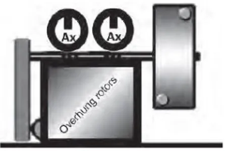
Unbalance – overhung rotors
In this case, the FFT spectrum displays a single 1xrpm peak as well, and the amplitude again varies proportional to the square of the shaft speed. It may cause high axial and radial vibrations. The axial phase on the two bearings will seem to be in phase whereas the radial phase tends to be unsteady. Overhung rotors can have both a static and couple unbalance and must be tested and fixed using analyzers or balancing equipment (Figure 3.4).
Figure 3.4 A belt driven fan/blower with an overhung rotor – the phase is measured in the axial direction
3.3
E
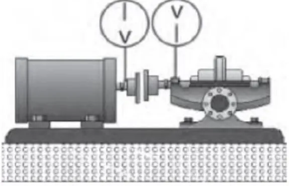
CCENTRIC ROTOREccentricity occurs when the center of rotation is at an offset from the geometric centerline of a sheave, gear, bearing, motor armature or any other rotor. The maximum amplitude occurs at 1xrpm of hte eccentric component in a direction through the centera of the two rotors. Here the amplitude varies with the load even at constant speeds (Figure 3.5)
29
Figure 3.5 A belt-driven fan/blower – vibration
In a normal unbalance defect, when the pick up is moved from the vertical to the horizontal direction, a phase shift of 90° will be observed. However in eccentricity, the phase readings differ by 0 or 180° (each indicates the straight line motion) when measured in horizontal and vertical directions. Attempts to balance an ec-centric rotor often result in reducing the vibration in one direction, but increasing it in the other radial direction (depends on the severity of the eccentricity) (Figure 3.6).
Figure 3.6 Eccentric rotor
3.4 B
ENTS
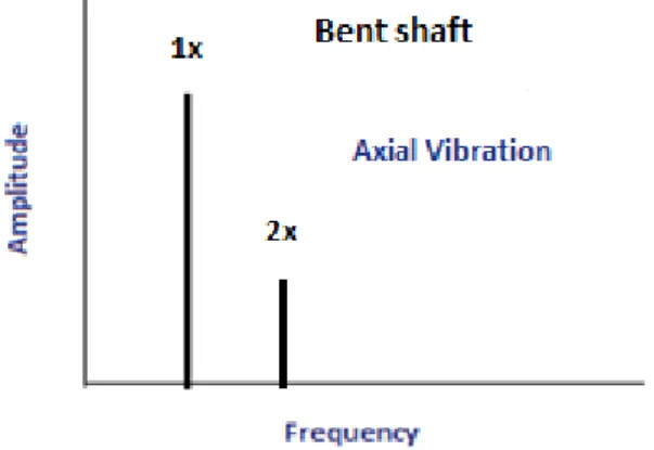
HAFTWhen a bent shaft is encountered, the vibrations is in radiala s well as in the axial direction will be high. Axial vibrations may be higher than the radial vibrations. The FFT will normally have 1x, 2x components. If the:
30
• Amplitude of 1x rpm is dominant then the bendi s near the shaft center (Figure 3.7)
• Amplitude of 2x rpm is dominant then the bendi s near the shaft end.
Figure 3.7 An FFT of a bent shaft with bend near the shaft center
The phase will be 180 ° apart in the axial direction and in the radial direction. This means that when the probe is moved from vertical plane to the horizontal plane, there will be no change in the phase reading (Figure 3.8).
Figure 3.8 Note the 180 ° phase different in the axial direction
3.5 M
ISALIGNMENTMisalignment, just like unbalance, is a major cause of machinery vibration. Some machines have been incorporated with self-aligning bearings and flexible cou-pling that can take quite a bit of misalignment. However, despite these, it is not uncommon to come across high vibrations due to misalignment. There are basi-cally two types of misalignment:
31
1. Angular misalignment: the shaft centerline of the two shafts meets
an angle with each other
2. Parallel misalignment: the shaft centerline of the two machines is
parallel to each other and have an offset
When a shaft has three or more bearings, for example when two machines are coupled together, there is a potential for misalignment, which can be parallel mi-salignment, meaning that one of the two shafts is displaced laterally, but still pa-rallel to the other, or angular misalignment, where the axis of one is at an angle to that of the other. Such misalignment introduces into the shafts bending deflec-tions, which are fixed spatially, but rotating with respect to the shafts. The induced bending moments thus depend on the bending stiffness of the shaft and have to be counteracted by forces at the bearings and the foundations.
3.5.1 Angular misalignment
As shown in Figure 2.9 angular misalignment primarly subjects the deiver and driven machine shafts to axial vibrations at the 1xrpm frequency. The figure is an single-pin representation, but a pure angular misalignment on a machine is rare. Thus alignment is rarely seen just 1xrpm peak. Tipically, there will be high axial vibration with both 1x, 2x rpm. However, it is not unusual for 1x, 2x or 3x to do-minate. These symptoms may also indicate coupling problem.
32
Figure 3.9 Angular misalignment
Figure 3.10 FFT of angular misalignment
A 180° phase difference will be observed when measuring the axial phase on the bearings of the two machines across the coupling (Figure 3.11).
33
Figure 3.11 Angular misalignment confirmed by phase analysis
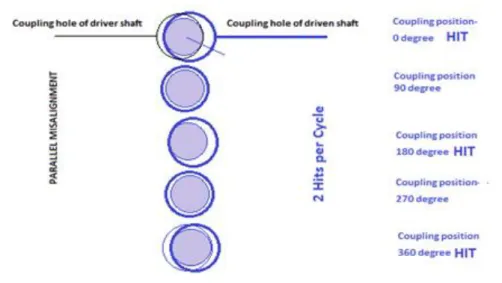
3.5.2 Parallel misalignment
Parallel misalignment results in 2 hits per cycle and therefore a 2x rpm vibration in the radial direction. Parallel misalignment has similar vibration symptoms com-pared to angular misalignment, but shows high radial vibration that approach 180° phase difference across the coupling. Pure angular Misalignment is rare and is commonly observed in conjunction with angular misalignment. Thus we will see both the 1x and 2x peaks. When the parallel misalignment is predominant, 2x is often larger than 1x, but its amplitude relative to 1x may often be dictated by the coupling type and its construction.
When either angular or parallel misalignment becomes severe, it can generate high-amplitude peaks at much higher harmonics (3x to 8x) (Figure 3.13) or even a whole series of high-frequency harmonics. Coupling construction will often si-gnificantly influence the shape of the spectrum if misalignment is severe (Figure 3.12).
34
Figure 3.13 FFT of parallel misalignment
Figure 3.14 Radial phase shift of 180° is observed across the coupling
3.6 M
ECHANICAL LOOSENESSIf we consider any rotating machine, mechanical looseness can occur at three locations:
1. Internal looseness
2. Looseness at machine to base plate interface 3. Structure looseness
3.6.1 Internal assembly looseness
This category of looseness could be between a bearing liner in its cap, a sleeve or rolling element bearing, or an impeller on a shaft. It is normally caused by an improper fit between component parts, which will produce armonic in the fft due to the non linear response of the loose parts to the exciting forces from the rotor. A truncation of the time waveform occurs, causing harmonics. The phase is often unstable and can vary broadly from one measurement to the next, particulary if the rotor alters its position on the shaft from one start-up to the next.
35
Mechanical looseness is often highly directional and may cause noticeably diffe-rent readings when they are taken at 30° increments in radial direction all around the bearing housing. Also note that looseness will often cause sub-harmonic mul-tiples at exactly ½ x or 1/3 x rpm (e.g. ½ x, 1 ½ x, 2 ½ x and further) (Figure 3.15 and 3.16).
Figure 3.15 loose internal assembly graph
Figure 3.16 Loose fit
3.6.2 Looseness between machine to base plate
This problem is associated with loose pillow- block bolts, cracks in the frame structure or the bearing pedestral. Figures 3.17 3.18 make it evident how ho-gher harmonics are generated due to the rocking motion of the pillow block with loose bolts.
36
Figure 3.17 Mechanical looseness graph
Figure 3.18 Mechanical looseness
3.6.3 Structure looseness
This type of looseness is caused by structural looseness or weaknesses in the machine’s feet baseplate or foundation. It can also be caused by deteriorated grouting, loose hold-down bolts at the base and distortion of the frame or base (known as soft foot).
Phase analysis may reveal approximately 180° phase shift between vertical measurements on the machine’s foot, baseplate and base itself (Figure 3.19). When the soft foot condition is suspected, an easy test to confirm for it is to loosen each bolt, one at time and see if this brings about significant changes in the vi-bration. In this case, it might be necessary to re-machine the base or install shims to eliminate the distorsion when the mounting bolts are tightened again.
37
Figure 3.19 Structure looseness
Figure 3.20 Structure looseness graph
3.7 R
OLLING ELEMENTB
EARINGA rolling element bearing comprises of inner and outer races, a cage and rolling ele-ments. Defects can occur in any of the parts of the bearing and will cause high frequency vibrations. In fact the severity of the wear keep changing the vibration pattern. In most cases it is possible to identify the component of the bearing that is defective due to the specific vibration frequency that are excited. Raceways and rolling element defects are easily detected. However the same cannot be said for the defects that crop up in bearing cages. Though there are many techniques available to detect where defects are occur-ring, there are no established techniques to predict when the bearing defect will turn into a functional failure. In an earlier topic dealing with enveloping/demodulation, we saw how bearing defects generate both the bearing defect frequency and the ringing random vi-brations that are the resonant frequencies of the bearing components. Bearing defect frequencies are not integrally harmonic to running speed. However, the following formu-las are used to determine bearing defect frequencies. There is also a bearing database
38
available in the form of commercial software that readily provides the values upon ente-ring the requisite beaente-ring number.
𝐵𝑃𝐹𝐼 =𝑁𝑏 2 (1 + 𝐵𝑑 𝑃𝑑 cos 𝜃) 𝑥 𝑟𝑝𝑚 𝐵𝑃𝐹𝑂 =𝑁𝐵 2 (1 − 𝐵𝑑 𝑃𝑑cos 𝜃) 𝑥𝑟𝑝𝑚 𝐹𝑇𝐹 =1 2(1 − 𝐵𝑑 𝑃𝑑cos 𝜃) 𝑥𝑟𝑝𝑚 𝐵𝑆𝐹 = 𝑃𝑑 2𝐵𝑑[1 − ( 𝐵𝑑 𝑃𝑑) 2 (cos 𝜃)2] 𝑥𝑟𝑝𝑚
Nb= Number of Balls or Rollers Bd=Ball/Roller diameter (inch or mm)
Pd=Bearing Pitch diameter θ=Contact angle in degree BPFI=Ball pass frequency inner BPFO=Ball pass frequency outer FTF=Foundamental train frequency BSF=Ballspin frequency (rolling element)
It is very interesting to note that in an FFT, we find both the inner and outer race defect frequencies. Add these frequencies and then divide the result by the ma-chine rpm – [(BPFI + BPFO) /rpm]. The answer should yield the number of rolling elements. Bearing deterioration progresses through four stages. During the initial stage, it is just a high-frequency vibration, after which bearing resonance frequen-cies are observed. During the third stage, discrete frequenfrequen-cies can be seen, and in the final stage high-frequency random noise is observed, which keeps broade-ning and rising in average amplitude with increased fault severity. In the following Figure the characteristic frequency of a Racer 3, 5, 5L and 7 Robot.
39
Figure 3.21 Characteristic frequencies of the bearing of axis 3
Stage 1 of bearing defect
The FFT spectrum for bearing defects can be split into four zones (A, B, C and D), where we will note the changes as bearing wear progresses.
These zones are described as:
Zone A: machine rpm and harmonics zone
Zone B: bearing defect frequencies zone (5–30 kcpm)
Zone C: bearing component natural frequencies zone (30–120 kcpm) Zone D: high-frequency-detection (HFD) zone (beyond 120 kcpm)
The first indications of bearing wear show up in the ultrasonic frequency ranges from approximately 20–60 kHz (120–360 kcpm). These are frequencies that are evaluated by high-frequency detection techniques such as gSE (Spike Energy), SEE, PeakVue, SPM and others. As Figure 3.25 shows, the FFT in case ra-ceways or rolling elements of the bearing do not have any visible defects during the first stage. The raceways may no longer have the shine of a new bearing and may appear dull gray.
40
Figure 3.22 Small defect in the raceways of a bearing
Stage 2 of bearing defect
In the following stage (Figure 3.26), the fatigued raceways begin to develop mi-nute pits. Rolling elements passing over these pits start to generate the ringing or the bearing component natural frequencies that predominantly occur in the 30– 120 kcpm range. Depending on the severity, it is possible that the sideband fre-quencies (bearing defect frequency ± rpm) appear above and below the natural frequency peak at the end of stage two. The high-frequency detection (HFD) tech-niques may double in amplitude compared to the readings during stage one.
Stage 3 of bearing defect
As we enter the third stage (Figure 3.27), the discrete bearing frequencies and harmonics are visible in the FFT. These may appear with a number of sidebands. Wear is usually now visible on the bearing and may expand through to the edge of the bearing raceway.
41
Figure 3.24 Wear is now clearly visible over the breath of the bearing
Stage 4 of bearing defect
In the final phase (Figure 3.28), the pits merge with each other, creating rough tracks and spalling of the bearing raceways or/and rolling elements. The bearing is in a severely damaged condition now. Even the amplitude of the 1× rpm com-ponent will rise. As it grows, it may also cause growth of many running speed harmonics. It can be visualized as higher clearances in the bearings allowing a higher displacement of the rotor. Discrete bearing defect frequencies and bea-ring component natural frequencies actually begin to merge into a random, broadband high-frequency ‘noise floor’. Initially, the average amplitude of the broad noise may be large. However, it will drop and the width of the noise will increase. In the final stage, the amplitude will rise again and the span of the noise floor also increases.
Figure 3.25 Severely damaged bearing in final stage of wear
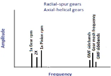
3.8 G
EARING DEFECTSA gearbox is a piece of rotating equipment that can cause the normal low fre-quency harmonics in the vibration spectrum, but also show a lot of activity in the
42
high frequency region due to gear teeth and bearing impacts. The spectrum of any gearbox shows the 1x and 2x rpm, along with the gear mesh frequency (GMF). The GMF is calculated by the product of the number of teeth of a pinion or a gear, and its respective running speed:
GMF= number of teeth on pinion x pinion rpm
The GMF will have running speed sidebands relative to the shaft speed to which the gear is attached. Gearbox spectrums contain a range of frequencies due to the different GMFs and their harmonics. All peaks have low amplitudes and no natural gear frequencies are excited if the gearbox is still in good condition. These contain information about gearbox faults (Figure 3.28).
Tooth wear and backlash can excite gear natural frequency along the gear mesh frequencies and their sidebands. Signal enhancement analysis enables the col-lection of vibrations from a single shaft inside a gearbox.
Cepstrum analysis is an excellent tool for analysing the power in each sideband family. The use of cepstrum analysis in conjunction with order analysis and time domain averaging can eliminate the ‘smearing’ of the many frequency components due to small speed variations.
As a general rule, distributed faults such as eccentricity and gear misalignment will produce sidebands and harmonics that have high amplitude close to the tooth-mesh frequency. Localized faults such as a cracked tooth produce side-bands that are spread more widely across the spectrum.