Optical power stabilization of a laser diode for qnd measurement

(1)

Scuola di Scienze

Corso di Laurea Magistrale in Fisica

OPTICAL POWER STABILIZATION OF

A LASER DIODE FOR QND

MEASUREMENT

Relatore:

Prof. Elisa Ercolessi

Presentata da:

Michael Chong

Sessione II

(2)

(3)

objects one has to struggle hard with experimental difficulties which, in real life, conspire to blur these simple pictures”

Haroche, S. Raimond, J.M. “Exploring the Quantum Atoms, Cavities, and Photons”

“It may sound crazy if you’ve learned too much quantum mechanics”

(4)

(5)

Abstract

L

Arealizzazione di stati non classici del campo elettromagnetico e in sistemi di

spin è uno stimolo alla ricerca, teorica e sperimentale, da almeno trent’anni. Lo studio di atomi freddi in trappole di dipolo permette di avvicinare questo ob-biettivo oltre a offrire la possibilità di effettuare esperimenti su condesati di Bose Einstein di interesse nel campo dell’interferometria atomica. La protezione della coerenza di un sistema macroscopico di spin tramite sistemi di feedback è a sua volta un obbiettivo che potrebbe portare a grandi sviluppi nel campo della metrolo-gia e dell’informazione quantistica.

Viene fornita un’introduzione a due tipologie di misura non considerate nei programmi standard di livello universitario: la misura non distruttiva (Quantum Non Demolition-QND) e la misura debole. Entrambe sono sfruttate nell’ambito dell’interazione radiazione materia a pochi fotoni o a pochi atomi (cavity QED e Atom boxes). Una trattazione delle trappole di dipolo per atomi neutri e ai comuni metodi di raffreddamento è necessaria all’introduzione all’esperimento BIARO (acronimo francese Bose Einstein condensate for Atomic Interferometry in a high finesse Optical Resonator), che si occupa di metrologia tramite l’utilizzo di con-densati di Bose Einstein e di sistemi di feedback. Viene descritta la progettazione, realizzazione e caratterizzazione di un servo controller per la stabilizzazione della potenza ottica di un laser. Il dispositivo è necessario per la compensazione del ligh shift differenziale indotto da un fascio laser a 1550nm utilizzato per creare una trappola di dipolo su atomi di rubidio. La compensazione gioca un ruolo es-senziale nel miglioramento di misure QND necessarie, in uno schema di feedback, per mantenere la coerenza in sistemi collettivi di spin, recentemente realizzato.

(6)

(7)

Introduction

S

Ince the early days of quantum physics the wave-particle duality that

char-acterizes the quantum world has inspired the formulation of thought exper-iments involving single particles and single photons to explore and exploit their quantum nature. Perhaps the most famous of these experiments, the photon box, animated the debate between Einstein and Bohr at the VI Congress of Solvay in 1930. Famous paradoxes have arisen from the quantum world, including the renowned Schrödinger’s cat. This example brings to our eyes the astounding con-sequences of the superposition principle applied to macroscopic systems and has inspired a theory of the decoherence phenomena. The Einstein Podolsky Rosen paradox, proposed in 1935, has lead to the formulation of hidden variables theo-ries and to Bell inequalities, and opened a debate about the principle of locality in quantum theory.

From the 1980s, scientific and technological improvement gave physicists the chance to implement real experimental setups to perform those thought experi-ments and to test many crucial points of quantum theory. In the field of atomic physics such improvements include ion traps, dipole traps and laser cooling. The 2012 Nobel Prize in physics to D.J. Wineland and S. Haroche "for ground-breaking experimental methods that enable measuring and manipulation of indi-vidual quantum systems"1 _{is the latest of a list of prizes for works in this field}

of physics, that embraces the study of cold atoms, of interferometry, metrology and the fundamental properties of the quantum world such as the measurement

1_{"The Nobel Prize in Physics 2012". Nobelprize.org.}

(12)

process.

Quantum nondemolition (QND) measurement, first proposed in the 1970’s for the detection of gravitational waves [14], is a special type of measurement pro-cess in which the uncertainty of the measured observable does not increase from its measured value during the subsequent normal evolution of the system. QND measurements allow to attain the true nature of quantum measurements: after the measurement process the system is collapsed in an eigenstate of the measured observable and subsequent measurements will find the system in the same eigen-state.

Recently single photons stored in a cavity have been measured without being ad-sorbed by a detector using QND measurements [44]; Fock states have been gen-erated in a controlled way in solid state systems [31]; non classical states of light have been prepared through feedback schemes that rely on QND measurements [51].

In the BIARO (French acronym for Bose Einstein condensate for Atom Inter-ferometry in a high finesse Optical Resonator) experiment, Rubidium atoms are trapped and cooled in a high finesse cavity. Ensembles of atoms are treated as pseudo spin system and the coupling with laser radiation allows to reach all op-tical BEC and to perform QND measurement of the population of the outermost electronic levels. Recently it has been proposed a theoretical scheme for the re-alization of spin squeezed states and Dicke states [54] using QND measurements and a feedback scheme to preserve coherence of a collective spin state [55] has been realized.

In such a dynamic context, the evolution of electronics, of microcontrollers and of fast responding and low noise systems, is of central importance and has been fundamental for the realization of many experiments that were unimaginable only fourty years ago.

Such a rapid development opens now the door to new discoveries and to the evo-lution of promising technology such as quantum computer. Furthermore weak measurements may allow the complete measurement of the wavefunction. The engineering of non classical states of matter and of light that may be used to

(13)

improve the quality of interferometers and of atomic clocks.

Outline of the thesis

This Master thesis work has been done at the Institut d’Optique in the Atom Optique group on the BIARO experiment.

The experiment focuses on quantum metrology and investigates several technolo-gies like: optical trapping of cold atoms, Bose Einstein condensates of Rubidium 87, weak measurement and feedback to protect an ensemble from the naturally occurring decoherence.

The first chapter is an introduction to measurements in quantum mechanics, starting from the postulates that define the measurement, following with the defi-nition of QND measurements and eventually treating the weak measurement.

The second chapter introduces to the dipole force, that may be used to trap atoms with lasers: starting from the atom-field interaction the dressed states ap-proach gives a great way to visualize what happens when single photons interact with single atoms treated first as two-level systems.

The third chapter is a review of theoretical aspects of optical dipole traps, common methods used to trap and techniques to cool neutral atoms. In particular red-detuned dipole traps for neutral atoms are treated.

The first three chapters serve as introduction for the in depth description of the BIARO experiment that is given in the fourth chapter. The experimental apparatus, the results concerning the realization of all optical Bose Einstein condensates and the engeneering of collective spin states through QND measurement are given, as well as the description of a feedback scheme recently developed.

My thesis work concerned the realization of a servo controller for the power of a fiber laser. The work has been driven by the necessity of a tuneable and stable optical power of a laser source aimed to improve QND measurements on trapped atoms. Chapter five is devoted to the conception and realization of such a device.

(14)

(15)

Chapter 1 MEASUREMENTS IN QUANTUM

MECHANICS

W

E know from any quantum mechanics textbook that when we perform a

measure on a system the wavefunction collapses on an eigenstate of the operator we are looking at. After collapsing the weavefunction evolves in time following the time tependent Schroedinger equation.

An example of measurement is the detection of a photon is using a photomulti-plier: in the process the photon is adsorbed. This kind of measurement is called a destructive measurement because the system we were looking at is not just pro-jected in the detected eigenstate of the operator, but essentially it is destroyed. In the extreme case where the light field may contain either one or no photons when we measure the presence of that photon we leave the field empty (see sec-tion 1.2). The measurement makes the system collapse in a state which is different from the one we measured.

In this chapter we will focus on the notion of measurement in quantum me-chanics starting from the postulates of quantum measurement in section 1.1. In the section 1.4 we define and discuss the weak measurement as defined by Aharonov [2] and as used later.

Finally in the last section we present and discuss the model of Quantum Non 5

(16)

Destructive1 _{measurement and how can we use it to obtain information from a}

quantum system without destroing it.

This chapter is meant to be a brief introduction at the theoretical aspects that lie behind the work of the BIARO experiment.

1.1 Postulates of measurement

We start by the postulates of measurement as given in the book from Cohen-Tannoudji and Laloe [20]. There it is possible to find a comprehensive discussion of the postulates, their physical interpretation and a detailed mathematical discus-sion2_.

First postulate: at a fixed time t0 the state of a physical system is defined by

specifing a ket |y(t0)i belonging to the state space S.

Second postulate: every measurable physical quantity A is described by an op-erator A acting inS; this operator is an observable.

Third postulate: the only possible result of a measurement of a physical quantity A is an eigenvalue of the corrisponding observable A.

Fouth postulate (discrete spectrum): when the physical quantity A is measured on a system in the normalized state |yi, the probability P(an)of obtaining

the eigenvalue anof the corresponding observable A is

P(an) = gn

Â

i=1|hu i n|yi|2

where gnis the degeneracy and the |uini form a set of orthonormal vectors

which form a basis in the eigensubspaceSnassociated with the eigenvalue

an.

1_{Often reported as quantum non demolition or QND.}

2_{Our discussion of the postulates is deliberately non-technical from the mathematical point of}

(17)

Fifth postulate: if the measurement gives the result an the state of the system

immediately after the measurement is the normalized projection onto the eigensubspace associated with an: pPn|yi

hy|Pn|yi.

Sixth postulate: the time evolution of the state vector |y(t)i is governed by the Schroedinger equation:

i¯hd

dt |y(t)i = H(t)|y(t)i .

It is the fifth postulate, otherwise described as the reduction of the wave packet, that stresses out the concept that goes under the name of projective measurement. The meaning is simple and at the same time extremely important: before perform-ing a measurement we should think in terms of probability to find a given result; this is due to the intrinsic nature of quantum mechanics and it is a consequence of the superposition principle3_{. But right after performing a measurement we do}

know in which particular state the system is: this is exactly the information we aquire through the measurement. If we could repeat it quickly enough we will get the same result. The time scale is fixed by the sixth postulate, the Schroedinger equation that tells us how the system will evolve with time.

1.2 Photodetection

Let’s describe what happens when we measure how many photons are there in a certain field. The standard way of doing this kind of measurement is in striking contrast with the projection postulate.

When we perform a photo-detection process applied to a field mode, the mea-sured quantity is the photon number operator ˆN = ˆa†_{ˆa. The eigenvalues of this}

operator are the the natural numbers and the eigenstates associated are the well

3_{Which is implicit in the first postulate, given that we provide a correct mathematical definition}

(18)

known Fock states with a definite number of photons. The counting of the pho-tons, however, relies on the conversion of the photons into electric charges through the photo-electric effect. Therefore the measured photons are destoyed in this pro-cess. The effect of the measurement is to project the state into the vacuum instead of projecting it into a random photon number state as required by the projection postulate. This kind of measurement does not "project" the state: it "demolishes" it. This kind of measurement takes therefore the name of demolition measure-ment.

The destruction of the state is not required by the measurement postulates; it is then natural to ask ourself if is it possible to perform measurements which do not demolish the state. A measurement that has the effects we expect from the postu-lates.

In the limiting case of a field that may contain either one or no photons we should ask ourself if is it possible to see the same photon more than once. This question leads us into the domain of quantum non-demolition measurement that we are going to treat in section 1.3.

1.3 Quantum Non Demolition measurements

A comprehensive introduction to QND may be found in [13]; from the histor-ical point of view it may be interesting to note that the first proposal of this kind of measurement were made in the context of gravitational wave detection in the 1970’s by Braginsky and Vorontosov.

Following the textbook approach of Haroche and Raimond [29] we start by stating the properties of a QND measurement: it is a detection process wich projects the state of the system into the eigenstate corresponding to the result of the measure-ment instead of erasing entirely the information of the state it has detected. The second essential feature in the definition of a QND process is the repeatability: two successive measurement should yeld the same result4_.

4_{Given that the system has not evolved in the meantime due to some kind of perturbation or a}

(19)

Let’s point out that this kind of measurement are the only measurement that fol-low strictly the postulates of measurement: this are the only true quantum mea-surements.

1.3.1 Conditions for QND

Here we state the conditions for a measurement to be QND.

Suppose we have a system S and that we want to measure an observable OS of

this system. The mechanism relies on the coupling of the system with a meter M that evolves among an ensemble of pointer states each "pointing towards" an eigenvalue of OS. The ensemble of this pointing states should form an eigenbasis

of an observable of the meter OM. The full Hamiltonian takes the form:

H = HS+HM+HSM, (1.1)

where the third term is the coupling between the system and the meter. The con-ditions for QND are that:

1. there must be some information about OSencoded in the pointer states after

the interaction: the system-meter interaction Hamiltonian must not com-mute with the meter observable.

[HSM,OM]6= 0.

This is a necessary condition that ensures that the interaction has some ef-fect on the evolution of the meter.

2. The measurement should not affect the eigenstates of OS. Often it is easier

to express this condition in a sufficient form5_:

[HSM,OS] =0.

5_{For a detailed discussion of this point, including the necessary form of this condition, refer to}

(20)

3. The measurement must be repeatable; excluding extremely fast processes we can require that the observable of the system should be an integral of motion for the free system Hamiltonian:

[HS,OS] =0.

The latter condition tells us that some quantities may never be measured in a QND way; the simplest exemple is the coordinate X of a free particle in a one dimen-sional motion: here the free Hamiltonian is proportional to P2and therefore does not commute with OS=X. In this situation we have a huge ’back-action’ of the

measurement on the system that makes it impossible to repeat the measurement and get the same result: if with the first detection we project the system into a posi-tion eigenstate, according to Heisenberg uncertainity relaposi-tion, the state has infinite momentum dispersion. Therefore during the time between two subsequent mea-surement we have an evolution of the system that have the effect of a complete dispersion of the results obtained for X.

1.3.2 Single-photon measurement

It may be useful to follow how a QND measurement is done in a specific sit-uation. In [29] there are several ones discussed both theoretically and from an experimental point of view. Here we report part of the discussion about the detec-tion of the presence of a single photon in a cavity using a Rydberg circular atom6 with a standard cavity QED setup using a Ramsey interferometer as in picture 1.1a.

The QND meter is a single Rydberg atom; three states with different principal quantum number |ei, |gi and |ii are involved. The coupling is provided by the resonant vacuum Rabi oscillation7 _{on the |ei ! |gi transition. The atom-cavity}

interaction time t is set for a 2p Rabi pulse on this transition.

6_{Rydberg atoms have high principal quantum number and in their circular configuration the}

atomic angular momentum may reach macroscopic values.

(21)

Figure 1.1: a) Atoms cross the cavity C one at a time; the cavity mode (shown in red) stores the field to be measured. The e, g and i atomic levels are shown in the inset. The cavity mode is resonant with the e ! g transition. Atoms are subjected in zones R1 and R2 (in green) to auxiliary pulses (frequencyn), quasi-resonant

with the g ! i transition (frequency ngi). Detector D, downstream, measures the

states of the atoms. b) Diagram depicting the interfering paths followed by an atom initially in g when there is no photon in the cavity mode. The atom travels between R1 and R2 either in g (violet line) or in i (blue line). The probability amplitudes associated with these two paths interfere, leading to fringes in the probability Pg

of detecting the atom in g whenn is scanned (shown at right). c) As b but when the cavity mode stores one photon. The atom, if in level g, undergoes a full re-versible cycle of photon absorption and emission, finally leaving the photon in C. In the process, the corresponding amplitude has undergone ap phase shift and the fringes are reversed (as shown at right). Image and caption taken from [44].

(22)

If the atom is initially in |gi and there is one photon the atom-field system un-dergoes a complete oscillation passing through |ei and comes back, up to a phase shift, to the initial state when the atom leaves the cavity. The state, depending on the presence of the photon, may undergo one of the following transformations:

|g,1i ! |g,1i; |g,0i ! |g,0i,

where |n = 1i (|n = 0i) represent the presence (absence) of a photon.

What is remarkable is that the presence of a photon produces a p-phase shift of the atomic state; the information is stored into the atom without destroying the photon making this a genuine QND process.

The atomic state |ii comes into play to detect this phase shift: the transitions from this level to the |gi level are far detuned from the cavity mode so that this state stays invariant passing through the cavity; it is therefore possible to use it as a phase reference.

The complete procedure to obtain the information about the cavity is the fol-lowing: first, ap/2 microwave pulse is applied to the atom before it enters the cavity, so as to put it in a coherent superposition of the |gi and |ii states:

|gi ! (|gi + |ii)/p2. (1.2) The atom then passes through the cavity and is later probed at the end exit of it using a secondp/2 pulse that completes the Ramsey interferometer setup realizing the transformations:

|gi !(|gi + ep if|ii) 2 ; |ii !

(|ii e if|gi) p

2 . (1.3)

Adjusting the microwave pulse around the |ii ! |gi transition it is possible to tune the relative phasef; the probability P_g|nof finding the atom in the state |gi depends on the presence of the photon in the cavity:

P_g|0= (1 cos(f))/2; (1.4a) P_g|1= (1 + cos(f))/2, (1.4b) If we choose the relative phase to be 0 it is easy to see that the probability to find the atom in the ground state is 0 if there are no photons in the cavity and 1 if

(23)

there is one. Therefore we have a way to detect the presence of the photon in the cavity. Is the state of the system destroyed after the measurement? When there are initially no photons in the cavity nothing happens: the atom was in the |gi state before entering the cavity and remains in the same state. The cavity remains empty. What happens to the photon if the cavity is not empty in the beginning? The Rydberg atom enters the cavity, absorbs the radiation and goes transiently through |ei before finally returning to |gi and releasing the photon. Therefore in the cavity there was a photon in the beginning and there remains one when the atom leaves the cavity.

Single photon cavity QND has been realized and a complete discussion of the (many) experimental subtleties may be found in Nouges et al 1999 [44].

Let’s stress out that this simple configuration is so effective only if the cavity is in the subspace spanned by |0i and |1i: if the cavity is allowed to be in a Fock state with more than one photon the 2p Rabi rotation is not exact anymore and there is probability of absorbing one photon after the complete rotation. We restrict to this simple situation which presents all the elements of a QND and we will not discuss the methods to realize a QND measurement of this type for a broader Fock subspace.

1.3.3 Standard Quantum Limit

One of the feature of QND measurement is that it makes possible to overcome the standard quantum limit (SQL). We know from the Heisenberg uncertainity principle that we cannot measure at the same time a pair of conjugate variables A and B with arbitrary precision:

DADB ¯h.

Anyway nothing prevents us from detecting one of the variables with arbitrary precision at the price of losing information on the conjugate. The SQL has to do with the continuous observation of a variable and in this section we discuss a simple example to introduce what this limit is following [13].

(24)

Suppose that the coordinate x(t) of the mass of an oscillator with eigenfre-quency w is continuously monitored. The value x(t) may be expressed by two quadrature amplitudes X1and X2related to x by:

x(t) = X₁cos(wt) + X2sin(wt). (1.5)

The measurement errors satisfy the uncertainity relation:

DX1DX2 _2mw¯h . (1.6)

The continuous monitoring of the coordinate is equivalent to the simultaneous measurement of the quadrature amplitudes with symmetrical uncertainityDX1=

DX2. If we substitute the symmetrical uncertainity condition in equation 1.5 we

obtain the standard quantum limit fo the coordinate of the oscillator: DSQL=

r ¯h

2mw. (1.7)

Different physical systems and observables have different SQLs and some exam-ples are given in [13] and in the references cited therein.

QND measurements allows us to extract information only on a single observ-able disturbing noncommuting ones precisely to the extent that provides satisfac-tion of the uncertainity principle. Using Braginsky’s words:

[...] the ideal QND measurement is an exact one: the meter does not add any perturbation, and possible variance is the consequence of the a priori uncertainity of the value to be measured.

1.4 Weak measurements

In this last section we introduce the concept of weak measurement first pro-posed by Aharonov et al. in 1988 in [2]. The idea of realizing this kind of mea-surement is becoming very common and there are several experiments nowadays that use this procedure to obtain information with a probe characterized by a re-duced strenght. An interesting and non technical review of these experiments may be found in [16] while a detailed one is [12].

(25)

Weak measurement is a generalization of the projective measurement that re-lies on a weak coupling between the system and the meter to gather some informa-tion about the system almost without perturbing it. The meter is usually a quantum object and to obtain the weak value of a quantum variable of the system we have to perform a strong measurement on the meter.

The standard measurement procedure has an Hamiltonian of the type [56]: H = g(t)QMAS, (1.8)

where g(t) is a normalized function with a compact support near the time of mea-surement t; QM is a canonical variable of the meter with conjugate variable PM8

and ASis the observable we want to measure.

In an ideal situation the initial state of the meter has a well defined PM value p.

The value of ASafter the interaction described by H is related to the final value of

PM.

In real situations we may assume the initial state of the meter to be a Gaussian in the QM and PM representations. Therefore, if the initial state of the system is

Âiai|AS=aii, the Hamiltonian (1.8) evolves the system to:

e iRHdte p2/4(Dp)2

Â

i

ai|AS=aii =

Â

i

aie (p ai)2/4(Dp)2|AS=aii. (1.9)

IfDp is much smaller than the spacing between the eigenvalues ai then after the

measurement we shall be left with the mixture of Gaussians located around ai

correlated with different eigenstates of AS. A measurement of PMwill then indicate

the value of AS.

What if theDp is much bigger than all ai? The final probability distribution will

still be a Gaussian but now we have a huge spread. The center of the Gaussian will be at the mean value of AS: hASi = Âi|ai|2ai. A single measurement like this will

give us almost no information because the spread of the Gaussian is much higher than the hASi.

If we want to measure the value of AS of a particle in an ensemble of N

par-ticles prepared in the same state we can reduce the relevant uncertainity by the

8_{They satisfy [Q}

(26)

factor 1/pN leaving unchanged the mean value of the average hASi. Enlarging

the number N we can obtain a measurement with the desired precision.

1.4.1 Postselection

For a sufficiently large ensemble, as said in the previous section, we are able to obtain the value hASi by taking the average of the outcome of the strong

mea-surement of PM.

We may now change the outcome of hASi by averaging on a particular

subensem-ble and taking account only of the values of PMof this part of the original

ensem-ble after the measurement has been done. We call the operation of chosing the subensemble a postselection. Surprisingly enough some postselections about the particles may yield values of hASi outside the expected range [min(ai),max(ai)].

The procedure of the measurement starts with a large ensemble of particles pre-pared in the same initial state. Every particle should interact with a separate mea-suring device. Then we perform the measurement wich selects the final state. In the end we take into account only the values of PM corresponding to the

postse-lected particles.

Consider an ensemble of particles with initial state |yii and a final state |yfi.

In between we switch on the interaction described in eq.1.8 with an initial state of the meter proportional to e q2_/4D2

. After the postselection the state of the meter (up to a normalization factor) is

hyf|e i

R_Hdt

|yiie q2/4D2⇠=hyf|yiieiq hy f |AS|yii

hy f |yii _e q2/4D2_. _(1.10)

The congruence holds if the spreadD is sufficiently small: D ⌧ maxn |hyf|yii|

|hyf|AnS|yii|1/n

. (1.11)

In the p representation the state of the meter after the postselection is approxi-mately

exp[ D2₍_{p h}yf|A|yii

hyf|yii ) 2_];

(27)

this state gives us the weak value for AS:

ASW ⌘ hyf|A|yii/hyf|yii. (1.12)

It is important to stress out that the uncertainty of p for each of the meters is much bigger than the measured value:Dp = 1

2D ASW therefore a single measurement

does not provide a precise information about the observable AS. But the average on

N system+meter devices allows us to come to the situation whereDp/pN ⌧ ASW

and is therefore possible to ascertain the value of ASW with arbitrary precision.

A discussion of the mathematics beheind the weak value may be found in the original paper by Aharonov [2] and in [3]. Weak measurement has opened the doors for a deeper understanding of the quantum world but has also introduced some strangeness that we won’t discuss here. For the interested reader there are recent experimental works (and open problems) about the possibility to measure the trajectories of particles passing through an interferometer [35] and about the complete measurement of a wavefunction [40]. In 1992 Lucien Hardy suggested a paradoxical thought experiment that uses weak measurements [28] and the first experimental realizations are now being published [58].

(28)

(29)

Chapter 2 DIPOLE FORCE

I

N this chapter we introduce the concept of dipole force raising from what is

called the lighshift of the levels of an atom due to strong coupling with a light field. The basic idea is that an electromagnetic field can be used to shift the energy levels of an atom; the energy shift is dependent on the intensity of the beam (and therefore, in a real situation, on the shape of the beam and the position of the atom inside it). Due to this dependance of the energy shift on the position the atoms in a laser beam experience a force dependent on their position and the detuning of the laser with respect to the atomic frequency.

In section 2.1 we introduce the results of the Rabi two-level problem as a starting point for the following sections. We then expose in section 2.2 the main results of the dressed states picture that are very useful to visualize radiation pressure and dipole force acting on atoms in a laser field.

2.1 Atom-Field interaction

Consider an atom in a radiation field: the time evolution of the system is given by the time dependent Schroedinger equation:

ˆ

Hy(!r ,t) = i¯h∂y(!_∂tr ,t), (2.1) 19

(30)

where ˆH is the total Hamiltonian for the atom in the field which is given by a field free, time indipendent, atomic part ˆH0and the interacting part ˆHi(t). The field free

part have eigenvalues En=¯hwnand eigenfunctionsfn(!r ) which form a complete

set that can be used to expand the solution of 2.1: y(!r ,t) =

Â

k

ck(t)fk(!r )e iwkt. (2.2)

If we substitute the expansion in 2.1, after a simple manipulation1 _{we get to the}

following system of equations that are equivalent to the starting equation: i¯hdcj(t)

dt =

Â

_k ck(t)H0jk(t)e iwjkt, (2.3) where H0 jk(t) = hfj| ˆH0(t)|fki and wjk= (wj wk).

2.1.1 The Rabi two-level problem

To evaluate the solution of such a system in the case of our interest we can make the following approximations:

1. consider an atom with the inner shells filled, so that only two atomic levels are available in first approximation; this means that in 2.3 we can truncate the sum just to two levels, ground (k=1) and excited (k=2). This gives the Rabi two-level problem first studied in [47].

2. If we use a narrow band laser (with angular frequencywl) as a radiating field

it is useful to make the rotating wave approximation (RWA) that consists in neglecting terms of the order 1/wl compared to terms of the order 1/d

where d = wl wa is the detuning of the laser compared to the atomic

resonance frequency.

3. We may consider the the electric field E (!r ,t) to be constant in space in the region of interest: the wavelenght is typically of the order of 102_nm

compared to the dimension of thefk(t) that usually are contained in a radius

 1nm. This results in the electric dipole approximation.

(31)

As a result of the approximation we can obtain the uncoupled differential equations for the cg(t) and the ce(t):

d2_c g(t) dt2 id dcg(t) dt + W2 4 cg(t) = 0, (2.4) d2_c_e_(t) dt2 +id dce(t) dt + W2 4 ce(t) = 0; (2.5) here we introduced the Rabi frequency2_{W defined as}

W = eE0 ¯h he|ˆr|gi,

where E0is the amplitude of a light field in the form of a plane wave propagating

in the z direction. To get an idea of what these equations imply let’s look at the solution for the simple initial conditions cg(0) = 1, ce(0) = 0:

cg(t) = ✓ cosW0t 2 i d W0sin W0_t 2 ◆ e+idt/2, (2.6) ce(t) = i_WW₀sinW 0_t 2 e idt/2. (2.7)

The generalised Rabi frequencyW0 _{is defined as:}

W0₌p_W2₊_d2_.

The solutions clearly suggest that the electron is oscillating between the two levels with frequqncyW0_{that increases with the detuning}_{d. The probability to find the}

electron in the exicted state is proportional to _WW022 that is the amplitude decreases

as we increase the detuning.

2.1.2 Introducing the Light Shifts

The effect of the field on the atom can be more subtle than what we considered until now. The energies En, eigenvalues of E0are no longer eigenvalues of the full

Hamiltonian due to off-diagonal terms in H0_.

2_{This definition of the Rabi frequency is made to be the real oscillation frequency of |c} k(t)|2in

(32)

If we evaluate the equations 2.3 using a time-indipendent perturbation H0

ge and

absorb the time dependence e iwkt into each coefficient c_k(t) we would get the

following set of equations3:

i¯hdc0g(t) dt =c0e(t) ¯hW 2 , (2.8) i¯hdc0e(t) dt =c0g(t) ¯hW 2 c0e(t)¯hd, (2.9) where the primed coefficients are related to the non primed ones by:

c0

g(t) = cg(t),

c0

e(t) = ce(t)e idt.

The energies of the ground and excited states, shifted by the field, are therefore found diagonalizing the matrix of the system to obtain:

DEe,g=¯h/2( d ⌥ W0). (2.10)

2.2 Dressed states picture

The eigenstates corresponding to the DEg,e are the so called dressed states

discussed in [20]; as in the whole chapter we will briefly report the results of our intrest: for an insightful discussion refer to [23].

We start by writing the Hamiltonian for the atom-laser coupled system ˆ

H = ˆHA+ ˆHR+ ˆV (2.11)

with the three terms in their second quantized version: ˆ

HA= P 2

2m+¯hwab†b; (2.12) here b = |gihe| and b†₌_{|eihg| are the lowering and raising operators.}

ˆ HR=

Â

l ¯hwl

a†_la_l, (2.13)

3_{There are different ways to get this result, including the rotating frame transformation;}

(33)

where a†_l and al are the creation and destruction operators of a photon in the

model amongst which there is l = l, the one corresponding to the laser field4_.

The interaction term is expressed (in the dipole approxmation and RWA) using the positive and negative frequency components of the electric field taken for the atomic average position r = hˆri5_:

E+_{(r) =}

Â

l El(r)al; E (r) =

Â

l E ? l(r)a†l.

The expression for the interaction is then just:

ˆV = !d ˙[b†E+_{(r) + bE (r)].} _(2.14)

In the following we neglect the kinetic term in the atomic Hamiltonian6_{. When the}

atom laser mode coupling is not taken into account (i.e. !d = 0) we get a picture which is easy to visualize:

"the eigenstates of the dressed Hamiltonian are bunched in manifolds En, n integer,

separated by the energy ¯hwl, each manifold consisting of two states |g,n + 1i and

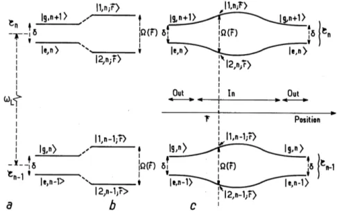
|e,ni"[23] separated by the energy ¯h(wa wl) =¯hd as in figure 2.1a.

Introducing the atom-laser coupling further splits the energy of states belong-ing to the same manifold. It is possible to re-define the (real) Rabi frequencyW(r) and to introduce a phasef(r) related by7 8_:

2

¯hhe,n|V|g,n + 1i = W(r)eif(r). (2.15)

4_{The electromagnetic field is quantized on a complete set of orthonormal field distributions}

El(r).

5_{A more complete treatment would use the position operator instead: the use of this}

semiclas-sical approssimation is valid as the extensionDr of the atomic wave packet is small compared with the laser wavelengthl.

6_{This is equivalent to solve the equations at a given point !}_{r .}

7_{The Rabi frequency defined in this way depends on the number of photons in the field. In a}

coherent laser field with Poissonian distribution and sufficiently large mean number of photons we can neglect the dependance and thus recover the previous definition.

(34)

Figure 2.1: Dressed states energy leveles. a) Shows the energy levels for two dif-ferent manifolds when the atom-laser mode is not taken into account. b) Effect of the laser-atom couplig on the energy levels. c) Position dependent energy levels in a gaussian laser beam: outside the beam we recover the situation of uncoupled states.. Image taken from [23].

The energies for the full dressed Hamiltonian are still folded in manifolds En(see

fig.2.1b) but the coupled levels are now shifted by the amount found in the pre-viuos section in eq. 2.10. It is now useful to sighty change the notation to better appreciate the dressed states formalism:

E1,2;n(!r ) = (n + 1)¯hwL ¯h

2 d ±W0(!r ) (2.16) corresponding to the eigenstates:

|1,n;!r i = +eif(!r )/2cos(q)|e,ni+e if(!r )/2_{sin(q)|g,n+1i;} _(2.17a)

|2,n;!r i = eif(!r )/2sin(q)|e,ni+e if(!r )/2cos(q)|g,n+1i. (2.17b) Here the angleq is position dependent and defined as:

cos(2q(!r )) = d

W0_(!_{r )}, sin(2q(!r )) =

W(!r ) W0_(!_{r )}.

(35)

The importance of this result is due to two different facts:

1. the dressed states are combination of the ground and excited states of the bare Hamiltonian;

2. in an inhomogeneus laser field both the energies and the states will depend on the position of the atom in the field (figure 2.1c depicts the situation for a gaussian beam).

2.2.1 Spontaneous emission

Spontaneus emission in the dressed picture allows to easily interpret the triplet structure of the spontaneus emission in terms of a princpial band (frequencywL)

and two sidebands (frequencywL± W0(!r )).

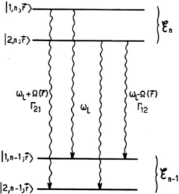
Since states |1,n;!r i and |2,n;!r i are superposition of the ground and excited states of the bare Hamiltonian we have four possible couplings when we con-sider the pair of manifolds Enand En 1that correspond to the three different

fre-quencies. The matrix elements between | j,n;!r i and |i,n 1;!r i are the di j=

hi,n 1;!r |d(ˆb + ˆb†)_{| j,n;!}_{r i:}

d11= d22=!d cos(q)sin(q)eif; (2.18a)

d12= !d sin2(q)eif; (2.18b)

d₁₂=!d cos2(q)eif. (2.18c) Here the diagonal terms correspond to the principal band as it is easy to infer from figure 2.2.

2.2.2 Radiation pressure and dipole force

Now that the states are defined and the possible interaction delined it would be possible to study the evolution of the density operatorr writing a master equa-tion for the populaequa-tionsPi(!r ) and coherencesri j(!r ) as function of the rates of

transfer Gi j (that are proportional, as one would expect, to the square of dipole

(36)

Figure 2.2: Spontaneus emission between dressed states and corresponding fre-quencies. Image taken from [23].

interested reader to refer to the many available references [18][23].

Here we are mainly interested at the effect in terms of force that the atoms experi-ence in a laser field so we report the result obtained for the average force9_which

is related only to the gradient of the atom-laser mode coupling: !_{f (!}_{r ) = hb}†_a

L—[!d EL] +ba†L—[!d ELq]i, (2.19)

it is then possible to recover the well known equation: !_{f (!}_{r ) =} ¯hW

2 i—f(rege if rgeeif)

¯h—W

2 (rege if rgeeif). (2.20) Here the termsreg=Ânhe,n|r|g,n + 1i and rge=Ânhg,n + 1|r|e,ni are the off

diagonal terms of the density matrix of the states of the bare Hamiltonian. The physical interpretation of the two terms in equation 2.20 is that the first part, proportional to the gradient of the phasef(r), is the radiation pressure term while the second one, proportional to the gradient of the Rabi frequencyW, is the

9_{Note that the results are still in the semiclassical approximation used before and the position}

(37)

dipole force which we are mostly interested in.

To get a view of how the dipole force behaves it is useful to express it as a function of the populations and coherences of the dressed states:

!_f

dip=¯h—W0(P2 P1) ¯hW0—q(r12+r21). (2.21)

Since the dipole force is related to the difference in the populations the effect is connected with the specific situation we are considering and the relative solution of the master equation for the density operator. The simplest case is the one for atoms at rest. It is important to notice that we are interested to cold atoms so that the atoms at rest situation is a good starting point and that the effects due to motion of the atoms10in the beam could be treated as corrections to this specific situation. Dipole force for atom at rest

If the atom is at rest we can replace the populations with their steady state valuesPst

i and express the dipole force as a function of the forces experienced by

the different dressed states—E1,2as:

f_dipst = Pst₁—E₁ Pst₂—E₂, (2.22) this is simply the mean between the two forces weighted by the probability of occupation. In terms of Rabi frequency and detuning it becomes:

f_dipst = — ✓ ¯hd 2 log(1 + W2 2d2) ◆ . (2.23)

Finally we can explain the connection between the sign of the dipole force and the sign of the detuning. Citing from [23]:

We would like to show ow the dressed-atom approach gives a sim-ple understanding of the connection between the sign of the dipole force and the sign of the detuningd = wL wa between the laser

and the atomic frequencies. If the detuning is positive the levels 1

10_{These effects include, but are not limited to, Doppler shift and variation of the force over a}

(38)

are those that coincide with |g,n + 1i outside the laser beam. It fol-lows that they are less contaminated by |e,ni than levels 2 and that fewer spontaneous transitions start from 1 than from 2. This shows that levels 1 are more populated than levels 2 (Pst

1iPst2). The force

re-sulting from levels 1 is therefore dominant, and the atom is expelled from high-intensity regions. If the detuning is negative, the conclu-sions are reversed: Levels 2 are more populated, and the atom is at-tracted toward high-intensity regions. Finally, ifd = 0, both states 1 and 2 contain the same mixture of e and g, they are equally populated (Pst

1 =Pst2), and the mean dipole force vanishes.

This gives account for the two different possibilities to use the dipole force to cool atoms: blue detuned lasers (di0) can be used to trap the atoms in the low intensity region of the beam whereas red dutuned one (dh0) do the opposite. We will further discuss the concept of dipole trap in chapter 3.

(39)

Chapter 3 OPTICAL DIPOLE TRAPS

I

Nthis chapter we discuss the way to use the dipole force introduced in chapter

2 to trap, and eventually cool by evaporative cooling, atoms using a detuned laser.

We will mainly refer to the article of Grimm et al. of 1999 [27] and Philips of 1998 [45] in the this chapter.

3.1 Trapping atoms

3.1.1 Dipole potential: another approach

The optical dipole force arises form the interaction between induced atomic dipole moment and intensity gradient of the driving field ([27]). Here we report briefly the main results wich are useful for our work. The reader is urged to note that while the approach of the previous chapter was useful to introduce and under-stand the nature of the interactions giving rise to the dipole force and the radiation pressure from a quantum point of view, now it may be convenient to think of the dipole moment !p in terms of the complex polarizabilitya and express its ampli-tude as

p =aE, (3.1)

(40)

where E is the amplitude of the electric field expressed in complex notation !_{E = ˆeEe} iwt_+c.c.

The interaction potential is therefore Udip= 1

2h!p !E it= 1

2e0c¬(a)I(!r ), (3.2)

where the angular brackets denote the time average over rapid oscillating terms and the intensity of the field is given by I = 2e0c|E|2.

The polarizability is a function of the damping rateG (corresponding to the spon-taneus decay rate from the excited level)[27]:

a = 6pe0c3_w₂ G/w0

0 w2 i(w3/w02)G

. (3.3)

The calculation ofG may be done in a classical way using the Larmor formula, in a semiclassical approximation (two level atoms + classical radiation) or even in a fully quantized approach. For most purposes with alkali atoms using the classical formula G = e2_w2

6pe0mec3 is enough, but for coherence with the previous chapter we

express it in the semiclassical approximation: G = w03

3pe0¯hc3|he| ˆd|gi|

2_. _(3.4)

In the usual RWA and in the limit of large detuning and negligible saturation (the excited level is far from being fully occupied) the expression for the dipole potential is derived as:

Udip=3pc 2 2w3 0 G dI(!r ) (3.5) and the scattering rate may be expressed as:

Gsc= 3pc 2 2¯hw3 0 (G d)2I(!r ). (3.6) Even in this semiclassical approximation we have recovered the dependance of the potential (and therefore of the force) on the sign of the detuningd. It may be useful to express the scattering rate as a function of the dipole potential:

Gsc=G_dUdip,

therefore a large detuning is often used to reduce the scattering rate keeping the depth of the trap constant.

(41)

3.1.2 Alkali atoms

Many experiments in atom cooling are done with alkali atoms. This is due to their rich internal structure that on one side blurs the simple ’two-level system’ picture, on the other offers plenty of opportunities for deeper investigation and sub-doppler cooling [43],[45] and [7]. At the BIARO experiment (see chapter 4) Rubidium atoms (87_{Rb) are used.}

The ns ! np transition, for a nuclear spin I = 3₂, has a complex scheme due to fine splittingDFSand hyperfine splittingDHFSfor each level (see fig: A.2). Let’s

remind that the energy scale is ¯hD0

FS ¯hDHFS ¯hD0HFS, where the prime refers

to the excited state.

For unresolved hyperfine splitting of the excited level (i.e. all optical detunings d DHFS), the ground state of an atom with total angular momentum F and

magnetic quantum number mF ’feels’ a light polarization potential [27]:

Udip(r) =pc 2_G 2w3 0 ✓2+PgFmF d2,F + 1 PgFmF d1,F ◆ I(r). (3.7) Here gF is the Landé factor, P refers to the polarization of the light (P = 0,±1,

for linearly and circularlys±_{polarized light) and the detunings}_d_1/2,F _{refer to the}

energy splitting between the ground state2S_1/2,F and the center of the hyperfine split of the the excited levels2_P

3/2and2P1/2respectively.

3.1.3 Blue-detuned and red-detuned dipole traps

We have seen in sections 2.2.2 and 3.1.1 that the sign of the dipole force and potential (as well as lightshift of the energy levels) depends on the sign of the detuningd. Traps realized with d > waare called red-detuned dipole traps while

the ones realized withd < waare called blue-detuned dipole traps.

The main difference is that red detuning provides a minimum of the potential in the high laser intensity region (e.g. the focus of the laser beam) whereas blue detuned light ’repels’ the atoms toward regions of low intensity (see Figure 3.1).

(42)

Figure 3.1: Dipole traps with red (left) and blue (right) detuning. For the red-detuned trap a Gaussian profile is assumed for the laser beam whereas a Laguerre-Gaussian LG01mode is taken for the blue-detuned one. Image taken from [27].

Red-detuned optical dipole traps

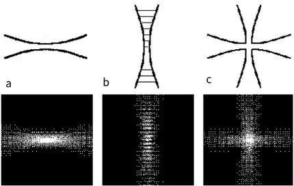
As stated in previous sections for a red detuning the focus of a laser beam provides the first example of a stable dipole trap; in fact it is the simplest one, but there are other possible solutions (see Figue: 3.2), like standing wave traps (that are useful to realize a 1D lattice of shallow potential minima) and crossed-beam traps on which we will focus more. Crossed-crossed-beam traps are used to resolve the anisotropy of the confinement that in a single laser beam trap is strong in the transverse direction and weak in the propagation direction.

It should be noted that with red detuned focused beam traps the attainable trap depth is of the order of mK, much smaller than thermal energy of the room tem-perature atoms: it is therefore necessary to pre-cool the atoms before being able to load them in such a trap.

Tipically the traps are loaded from pre-cooled atoms trapped in a magneto-optical trap (MOT); the specific configuration of the MOT(s) and their position with re-spect to the dipole trap depend on the purpose and on the creativity of the exper-imenters. We will briefly describe the configuration of the BIARO experiment in section 4.1.

After loading a crossed-beam trap it is possible to use it to perform evaporative cooling (see [1] for a ’proof of principle’ experiment with Na atoms), a technique that is fundamental to increase phase-space density, that has been the key to obtain Bose-Einstein condensates [4], [24]. In order to achieve evaporative cooling the

(43)

optical power of the laser used for the trap is ramped down to allow the atoms with higher thermal energy to escape from the trap. After thermalization of the atoms remaining in the trap, the temperature is decreased and the phase-space density may increase.

Figure 3.2: Dipole traps types. a) Single focused beam trap. b) Standindg wave trap. c) Crossed beam trap. Image taken from [27].

Blue-detuned optical dipole traps

Blue-detuned light offers the possibility to realize traps in which the atoms are stored in a ’dark’ spot, therefore reducing the effects of light on the sample atoms. In particular there is no or little light shift of the energy levels, photon scattering is greatly reduced and losses due to interaction with light are limited.

There are however some disadvantages in realizing these kind of traps, mainly due to the fact that the laser beam repels the atoms and is necessary to realize ’walls’ around the dark area in which the sample is to be confined.

The balance of these two aspects makes blue-detuned dipole traps efficient in the situation of hard repulsive optical walls or large potential depth for tight confining (U kBT ). For an extensive description of the possible geometries and means to

(44)

realize a trap using blue detuned light refer to [27] or [43].

3.2 Cooling methods in dipole traps

In this section we briefly review the most used methods for cooling samples in dipole traps. We remind, for historical reasons, that atom cooling methods have been enhanced greatly in the late eighties and in the nineties of the 20th century and that the field is still growing, though at a slower pace.

The first big step has been the developement of Doppler cooling: this method is "based on cycles of near resonant absorbtion of a photon and subsequent spon-taneus emission resulting in a net atomic momentum change per cycle of one photon momentum ¯hk with k = 2p/l denoting the wave number of the absorbed photon"[27]. Since spontaneus emission give rise to heating due to momentum recoil, the limit in reacheable temperature is given by the equilibrium between heating and cooling. Theoretical treatment of Doppler cooling relies on the simple two-level atom picture. The minimum temperature reacheable with this method is called Doppler temperature kBTD= ¯hG/2 and is of the order of 101 2mK, just

enough to load a dipole trap.

To reach sub-Doppler temperatures one has to exploit the complex structure be-yond the two-level picture; polarization gradient cooling is realized with standing waves with spatially varying polarization and relies on optical pumping between Zeeman sublevels of the ground state. The most-famous version of this method is probably the "Sysiphus cooling" [23] in which an atom loses kinetic energy climb-ing up the dipole potential induced by a standclimb-ing wave with varyclimb-ing polarization; when the polarization of the wave changes froms+ _to_{s the light shift of two}

Zeeman sublevels must change in a correlated way in order to make a moving atom runs up a potential hill more often than it runs down. The net effect is that the loss in kinetic energy is greater than the gain. For a comprehensive description and illustration of this method see [19] or [45]. Exploiting Sysiphus effect allows to reach temperatures of the order of 10Trecwhere the recoil temperature, defined

(45)

as

Trec=¯h2k2/m, (3.8)

is the gain in temperature associated with the kinetic energy gain due to the emis-sion of one photon. For alkali atoms Trecis of the order of theµK, being equal to

0.36µK for Rubidium 87 that is used in the BIARO experiment.

To reach sub-recoil temperatures one has to introduce an absorbing mecha-nism that is sensible to atom velocity; the idea is to make the atoms with ve-locity close to zero dark to the absorbtion-emission mechanism. Raman cooling [33] is realized with Raman pulses from two counterpropagating lasers that trans-fers atoms between two ground levels |g1i and |g2i transferring 2¯hk momentum

in each absorbtion. Adjusting frequency width, detuning and propagation direc-tion one can tailor pulses that excite all atoms but the one with velocity close to zero. Spontaneus emission from excited atoms in |g2i, being random in direction,

brings atoms back to |g1i leaving a bigger fraction of the sample with (almost)

zero velocity. Repeating the cycle allows to accumulate atoms in a small veloc-ity interval around v = 0 thus cooling the sample. Raman cooling allows to reach sub-microkelvin temperature but requires pre-cooling with another mechanism being effective on samples with starting temperature of the order of few tens of microkelvin.

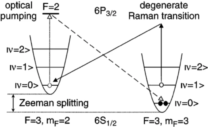
Resolved-sideband Raman cooling

Resolved-sideband Raman cooling is a tecnique developed first for laser cool-ing in ion traps and later adjusted for trappcool-ing neutral atoms [57]. The requirement for this method of cooling is to have a strong confinement of the atoms in at least one dimension, with oscillation frequency wosc large enough to be resolved by

inelastic Raman transitions between two ground levels. The degeneracy of the ground level is usually resolved with the aid of a small magnetic field, therefore the splitting between the ground levels is of the order of a Zeeman splitting. The atomic motion is described by a wavepacket formed of a superposition of vi-brational states |ni; in the Lamb-Dicke regime (rms size of the wavepacket small compared with the wavelenght of the cooling transition) almost all

(46)

absorbtion-spontaneous emission cycles returns to the same vibrational state (Dn = 0). To per-form resolved-sideband Raman cooling one must repeat cycles of Raman pulses tuned to excite transitions with Dn = 1 followed by optical pumping into the initial state withDn = 0. The net effect the motional ground state |n = 0i is selec-tively populated since it is the only state that is dark to the Raman pulses.

Figure 3.3: Resolved-sideband cooling scheme using the two lowest ground states of Cs atoms. Image taken from [57].

(47)

Chapter 4 THE BIARO EXPERIMENT

I

Nthis chapter we will describe the experimental setup and the purpose of the

BIARO experiment. In section 4.1 we will give a brief description of the appa-ratus, the cavity and the cooling methods used in the experiment. In the subsequent section, 4.2 we will introduce Bose Einstein condensation and describe how it has been possible to reach it in the BIARO experiment. Section 4.3 is devoted to how to perform a QND measurement in the experiment; from the theoretical analysis of such measurements it has been predicted the possibility to produce non clas-sical atomic states using QND measurements [54]. These kind of measurements have been recently used to perform feedback which is a mean to fight naturally occurring decoherence of a coherent spin state[55].

Section 4.4 is a brief discussion of the compensation of the differential light shift induced by the trapping radiation on the levels involved in the D2 transition.

The setup, the theoretical analysis and all the experimental results reported in this chapter have been realized in the years from 2009 by the scientists that have worked on it until now. The description of the state of the experiment is important to understand the purpose of the work described in chapter 5.

(48)

4.1 Experimental setup

In this section we will describe the setup: the cavity, the trapping and the cooling methods.

The experimental apparatus is composed of two chambers: the first is kept under high vacuum (pressure below 7⇥10 8_{mbar) and a 2 dimensional}

magneto-optical trap (MOT) is operated and used as a source1 _{of pre-cooled atoms. The}

science chamber is kept under ultra-high vacuum (pressure below 10 9_{mbar) and}

contains the coils for a 3D MOT as well as the crossed optical cavity. Experiments are realized in the science chamber at the center of the cavity.

Technical details on this part may be found in [8] [9] [10] [37] [53] [54] [55].

4.1.1 The high finesse cavity

Here we report a description of the main properties of the cavity; the full char-acterization of the cavity is reported in [8] and [52]

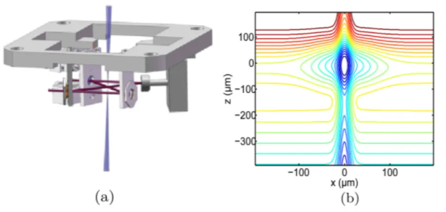
The cavity is in a butterfly configuration (see fig 4.1), an ingenious idea to provide high trapping (i.e. deep potential) with low power laser. The geometry of the cav-ity allows the realization of a crossed-beam dipole trap (see section 3.1.3 and Fig: 3.2).

The cavity is made up of four mirrors placed at the corners of a square with a diagonal of 90mm; two mirror mounts are completely fixed while one is actuated by piezoelectric actuators, which allow for a coarse alignment of the cavity. The last mount is a piezo-actuated three-axis nano-positioning system with a maximal angular displacement of 2mrad and a translation of 50µm. It is used to finely ad-just the cavity crossing angle and dynamically control the cavity length [8]. The four mirrors of the cavity are highly reflecting at both 1560nm and 780nm. The free spectral range (FSR) of the cavity is 976.2MHz and the cavity’s full width at half maximum (FWHM) linewidth isg = 546kHz at 1560 nm.

The finesse2_{of the cavity has been studied a priori for the two resonating} wave-1_{The source of atomic background pressure is the vapor pressure of a 1g}87_{Rb sample.}

(49)

Figure 4.1: a)Scheme of the butterfly cavity.b)The inner vacuum setup with the suspended cavity and the coils generating the MOT magnetic field; image taken from [9]

Figure 4.2: Tomographic images of the optical potential. The images are obtained setting the probe frequency to different detuningD with respect of the D2line. The

images represent atoms with energy levels lightshifted in a position-dependent manner. Atoms which are sensitive to higher detuning are experiencing a higher lightshift i.e. they are deeper in the optical potential. Image taken from [9].

(50)

lenghts and then measured [9] for 1560nm obtaining F1560=1788.

The trapping laser radiation at 1560nm is injected in the cavity and excites the fundamental transverse electromagnetic (TEM00) mode: both the magnetic and the electric field are perpendicular to the direction of propagation3_{. Tomographic}

images of the optical potential have been obtained with light-shift tomography [15]. The 1560nm laser has been locked to the cavity using a Pound-Drever-Hall technique [25] that allows to fast correct the frequency with an acousto-optic mod-ulator in double pass [8] [9]. Frequency stabilization of the trapping radiation has been improved using serrodyne modulation as described in [37]. The 780nm prob-ing radiation is obtained by doublprob-ing the frequency of the trappprob-ing laser.

Higher modes of the cavity

The use of phase masks allows an efficient injection of modes of the cavity different from the fundamental TEM00. In particular in [10] there is the full de-scription of the method used to lock the 1560nm laser to the TEM10 and TEM20 modes. These modes may be used in the future to trap atoms in a well defined lattice, cool the atoms down to the BEC temperature (see section 4.2) and obtain a lattice of BECs. This geometry can be superimposed to the fundamental mode of the cavity during an experimental sequence: therefore it may be used to split the condensate trapped in the fundamental mode and perform experiments on conden-sates in each lattice site and then regroup the condensate by removing the higher modes. It may be possible in the future to exploit this feature to perform high precision atomic interferometry using the BECs [8].

4.1.2 The trapping

The Gaussian profile of the 1560nm beam that excites the fundamental mode of the cavity produces a position dependent lightshift on the levels of our interest,

2_{The finesse F of the resonator is defined as the ratio of the FSR and the FWHM of a resonance}

for a specific resonance wavelength.

3_{See, for instance, [36] or R. Paschotta Encyclopedia for Photonics and Laser Technology,}

(51)

Figure 4.3: . Image taken from [9].

that realize an optical dipole trap. Considering only the relevant D1and D2

tran-sitions, the ground level 5S1/2 is downshifted for a maximum of the intensity so

atoms will be trapped in the ground state at the center of the Gaussian beam. The 5P3/2state would be, if we consider only the D lines, blue-shifted and would expel

the atoms at the maximum of the intensity. Since the 5P3/2! 4D5/2,3/2transitions

are at 1529nm it is important to take them into account; for these transitions the trapping radiation is red-detuned so the 5P3/2level is red-shifted; the proximity of

these 1529nm resonances makes the light shift on the 5P_3/2level large compared to the one of the ground state resulting in a differential light-shift of the relevant level as shown in Fig: 4.4. The trapping of the atoms is done in three steps: using the 2D MOT an array of cold atoms it is realized and eventually directed towards the 3D MOT [52]. The array of cold atoms is then trapped in a 3D MOT centered on the cavity crossing region (and 3mm above the 2D MOT jet to avoid direct collisions with thermal atoms). In this situation it is possible to obtain an atomic cloud of a few 109_{atoms after 3 seconds of loading [9].}

The last step, described in [9], is the transfer of the atoms from the 3D MOT to the dipole trap realized with the trapping radiation at 1560nm.

After the loading sequence about 25 ⇥ 106 atoms are trapped at the crossing re-gion of the dipole trap at a temperature T = 230µK. The number of atoms in

(52)

Figure 4.4: . Image taken from [8].

the trap decreases with exponential behaviour (lifetimet = 6.7s); the temperature was measured to be constat in the dipole trap, meaning that the trap itself do not heat the atomic sample: the heat is exactly compensated by the energy lost trough evaporation of the most energetic atoms.

4.1.3 Cooling

The optical cooling of the atomic sample requires two lasers. The first one is tuned of about 3G on the red side of the cycling transition |F = 2i ! |F0₌_3i;

the photon is absorbed with higher probability from the direction against velocity of the atom. The momentum transfer gives a kick in the opposite direction slow-ing down the atom. Since there is non zero probability to excite the transition |F = 2i ! |F0=2i and since from |F0=2i the atoms can decay to the ground level |F = 1i which is dark to the cooling laser, a repumper tuned on the transition |F = 1i ! |F0=2i that repumps the atom on the |F = 2i level is used [8] [53]. The two lasers are extended cavity laser diode: the repumper is locked to the hy-perfine |F = 1i ! |F0₌_{2i transition through frequency modulation spectroscopy}

(53)

and the cooling laser is frequency locked to the repumper. The frequency of the cooling laser may be changed with respect to the atomic transition and this is es-sential to load the optical dipole trap from the MOT. The two lasers used for the cooling are injected in a fiber cable and used both for the 2D and the 3D MOTs [8], [9], [53].

Evaporative cooling

To obtain Bose Einstein condensation (see section 4.2) in the dipole trap, evap-orative cooling is used. The quantum degenerate regime for the BEC requires small interatomic spacing in the sample which is obtained with high trapping fre-quency. It is then important to measure the frequencies of the trap to define an op-timal ramp for the evaporative cooling: the chosen ramp must result in increased phase space density of the sample. A theoretical analysis of the frequencies of the trap is reported in [8] and [53].

Measuringthe trap frequencies

It is worth citing two experimental methods to measure the trap frequencies: the first exploits parametric heating whereas the second measures the modes of oscillation after a sudden change of the geometry of the trap [53].

To measure the trapping frequencies exploiting parametric heating a sinusoidal modulation is applied on the trapping depth after loading the trap. After a fixed number of oscillation (500 in the context of BIARO) the number of atoms at the center of the trap is measured. Sweeping over a range of frequencies it is possible to find the resonance frequency, characterized by important losses in the number of atoms. In parametric heating the resonance frequency is twice of the frequency of the system (in our case of the trap). The horizontal frequencywx=wyis found

to be equal to 700Hz when the intra-cavity power is 240W [53].

When the frequency is measured by changing the shape of the trap, the idea is to suddently increase the intra-cavity power (up to 240W in the context of BIARO) and observe the oscillation of the size of the atomic cloud: the frequency of this

Optical power stabilization of a laser diode for qnd measurement