Youth poverty after leaving parental home: does parental income matter?

Youth Poverty after Leaving Parental Home in Southern

European Countries:

Does Parental Income Matter?

Lavinia Parisi

29th May 2006

Abstract

Researchers have now started to look at youth poverty as distinct from child poverty. However none has focused on the intergenerational transmis-sion of youth poverty in European countries. Using four countries for which there are data from the European Community Household Panel, this paper analyses the link between the poverty status of youth after they have left home and the economic status in the family of origin. We adopt a wider age range than in most studies on youth poverty, i.e. between 18 years old and 34. The sample is constitute by youth that have left home as part of a couple. The evidence shows that in Southern European countries there is a negative association between parental income and leaving home as part of a couple: the poorer the family of origin, the less likely is youth to leave home as a couple, so we use a sample selection model (Heckman Probit) to model the probability to be poor after leaving home, where the selection equation is the probability to leave home to live with a partner. We esti-mate the model separately for each country and also pooling the countries all together using some interactions. The main results show that there is no sample selection bias for any of the countries. The outcome is not different from the one obtained by fitting the Probit and selection models separately. There is a strong effect of the economic status of the family of origin on the probability to be poor in after they have left home, except for Greece. There are not great differences between Italy, Spain and Portugal, even if the intergenerational transmission of poverty seems to be stronger in Spain.

Contents

1 Introduction 3

2 Youth poverty, leaving home and the intergenerational poverty

model 7

3 Method 11

3.1 The sample selection model . . . 12

4 Data 15

4.1 Selection of the analysis sample . . . 15

4.2 Definition of key variable: parental income . . . 16

4.3 Descriptive statistics for sample . . . 18

5 Model estimates and implications 21

1

Introduction

In recent years many studies have started to focus the link between youth and the previous generation. However, only few researches have been looked at the youth poverty status, and even less has been focused on the inter-generational transmission of poverty in European countries. In this paper we analyze the relationship between income of parent and poverty status of their children while also taking account of several individual and territorial characteristics that are not often used in the literature i.e. features of family

1_{, neighbourhood and area of residence that we assume are correlated with}

the lack of material resources.

The definition of ‘youth’ in this paper is slightly different from the one usually used in literature. Youth usually are ‘those who are no longer chil-dren, but who belong to an age group many of whose members have not yet completed all the processes of transition to adulthood’ (Aassve et al., 2005a, p. 1), so youth is usually considered as starting around 15 years old and ending around 25. We are not interested in age limits but on the process of transition to adulthood.

In this paper the final transition to adulthood does not occur when young people leave their parents’ home to form a stable cohabitation and so does

1_{A family comprises a group of people with parent links consisting of married or}

cohab-iting couple, single male or female, with or without children. The family also can include grandparents or grandchildren living at home. The household is a quite wider concept including different unit leaving in the some house but with not parental links i.e. a house-hold can comprise a family of a married couple with one child plus a student renting a room in the house (see Atkinson 1990). In this work we refer to family, strictly speaking

not mark the end of youth independently of the age at which that occurs. We focus on Southern European countries (henceforth SEC), where the decision to leave home occurs later than the other European countries. Ac-cordingly to Iacovou (2004, p.27), the young people in all southern/catholic countries are similarly slow to leave home: for men, the mean is 30year old in Italy and 28 years old in Spain Portugal and Greece; for women, the mean is 27, in Spain and in Italy, 25 and 23 in Portugal and Greece respectively.

There are several reasons why Southern European youth take longer to leave home. First, the rate of unemployment is higher than the European mean; second, the housing prices are high and third, even for those young individuals who already got a job or formed a stable cohabiting union (even marriage), the informal care provided by their parents may lead them to remain at their parents’ home. Manacorda Moretti, (2005) find evidence for this in Italy stating that parents value greatly to have children at home longer and so they offer income transfers to keep their own children at home as long as possible.

Moreover, the evidence in these countries shows that the age of leaving home and partnering tend to occur at the same time. As Iacovou (2004) argues, leaving home as a single person should be distinguished from leaving home as a couple. For all these reasons we adopt a wider age range than in most studies on youth poverty, i.e. we analyze youth aged between 18 years old and 34, where both the lower and the upper age limits are higher respect. The paper considers the hypothesis that young people prefer to live on

their own but they delay leaving home because they consider this to jeopar-dies their wellbeing: stay at home it is a protection against poverty.

Many studies, in fact, find a strong link between leaving home and youth poverty emphasizing that leaving home is more important to explain poverty among young people than other factors like employment, presence of children or cohabitation. Aassve at al. (2005b) find that youth delay leaving home because they know they are more likely to enter poverty than those who decide to stay in parental home.

In Italy, not only the poverty risk is a very important reason for delaying, but also the stayers have a further incentive as their well being increases given the income transfers they receive from their parents (Manacorda, Moretti, 2005). In Spain, for youth in the late twenties compare the ones in the early twenties, the poverty risk is lower: the delaying of leaving home could be due to the fact that they are economically supporting their parents (Aassve et al. 2005b).

Regarding the leaving home decision we assume that there are other fac-tors beyond youth poverty which are correlated with the economic status of the family of origin. We consider that the lack of material resources in the family of origin influences both the choice of neighbourhood in which the family lives and the networks in the labour market. On the other hand, for the youth living in a better-off family, delaying the decision to leave home can increase the probability to find a better job, and so to have more eco-nomic independence. So, we assume that the intergenerational transmission

of poverty is fostered by the low level of wellbeing that youth faces during is childhood and adolescence.

As we stated before, the evidence shows that in southern European coun-tries there is a negative association between parental income and leaving home as part of a couple, in other words the more poor the family of origin is, the less likely youth are to leave home as a couple. This suggests a po-tential sample selection bias because there are some unobserved factors that determine the inclusion on the sample (youth that have left parental home) and, at the same time, affect the outcome of primary interest (the youth poverty status). To address this issue we use a standard sample selection model i.e. Heckman probit.

The paper is structured as follows. In the first section we describe the main findings of the literature on youth poverty and the leaving home decision in Europe. This section, also provides a framework to analyze the intergen-erational transmission of poverty. In the second section we summarize the data used in the analysis and describe the sample and the methods. In the third section the results are presented. Finally, the last section concludes. The appendices include detailed information about the sample constructions and the variables of interest.

2

Youth poverty, leaving home and the

inter-generational poverty model

Despite of the large body of research on poverty on particular age groups (in particularly children and elderly) there are very few studies on poverty among youth as distinct from child poverty.

The first issue that arises is the very definition of youth that varies widely across countries, and there is no strong agreement about when a child should be considered as belonging to the youth group. Therefore, it is not surprising that studies on youth poverty or youth outcomes start with the issue of youth definition. There is consensus in considering that youth are individuals who have not yet completed all the processes of transition to adulthood.

However, nowadays it is unclear in which moment a young people has completed all the steps of the transition to adulthood. It is well established that the transition include five steps (i.e. completing education, finding a job, leaving the parental home, forming a stable cohabiting union and having chil-dren)but there is room to discussion about whether they are chronologically ordered. Often, the transition to adulthood is not a smooth process and some steps occur later and later in the life; some others can take place si-multaneously, women may make the transition differently from men. For all these reasons we can not find a standard definition of youth, especially if we compare different countries.

policy, a definition of youth based on upper and lower age limits: the United Nations defines young people the individual aged between 15 and 24 years old, as well as the European Union. The more appropriate way to address this issue is to find a definition according to the analysis that one is going to do, and above all according to the features of the countries that one is going to analyse.

As we stated before, there are very few studies on youth poverty. Among comparative studies the most recent one is the paper written by Aasve, Ia-covou and Mencarini (2005) on the youth poverty in Europe. They review the literature on youth poverty and state that almost all the studies on poverty among young individual are based on two datasets: the Luxembourg Income Study (LIS) and the European Community Household Panel (ECHP). Us-ing data from ECHP, they find that in Europe the SEC have the highest rate of poverty in general, but compare with the UK only in Italy the youth poverty is higher. Moreover, in these countries there is no peak rates in any age associated with leaving home. In fact in the SEC the difference in poverty rates between those living at home and those who have left home is the lowest when compared to the other European counties. Plotting the gap in poverty rates between those at home and those who have left home against the proportion of youth that have left home, they found a strong positive relationship between the two variables considered. In other words, in a country where the proportion of youth that have left home is high, the gap in the poverty rate is bigger.

Smeeding and Phillips (2002) use seven nations for which there are data from LIS to portray the level of economic independence among youth (aged 18-32). They choose the seven nations according to their previous studies and to have a wide range of countries reflecting different welfare regimes and geographical position. They use, as a key of interpretation, the classification of Esping-Andersen (1990) for welfare state as they address the issue of so-cial benefits and economic transfer in contrast to the economic insufficiency. Among the Mediterranean countries they select Italy. They show that look-ing at the economic independence archived through market work (even if it is combined with government transfer) the young Italian men experience the lowest percentage of ”full-time and full-year work” . They also show that neither Italy men nor women can earn enough to escape from poverty. The percentage of young adults able to support a family of three with their earn-ings is even lower when compared to the other countries. They stress the role of the Italian labour market saying that ‘the fact that young Italian men do so poorly likely reflects that fact that labour market opportunities are fewer and less well paid and that the institution of the Italian labour market are likely to favour older men’ (Smeeding and Phillips, 2002 p. 8).

Canto’-Sanchez and Mercader-Prats for Spain analyse economic poverty among children and youth aged between 18 and 29 in the 90’s. They find that children are the age group with the highest risk of poverty in contrast with youth that show the lowest (7.6%). The risk of poverty rises drastically for children living in a household headed by a youth. The regression presented

confirm this analysis showing that poverty is lower for youth aged 18-29 compared to the whole population even if it is slightly higher for older youth (aged 25-29) than for younger youth (aged 18-24). They explain in two different ways the low risk of youth poverty: first of all 80% of youth live with their family, in fact poverty is higher for the youth who have left their parental home (this can show the hypothesis that live in parental home it is the most important protection against poverty). Secondly, the 60% of youth in Spain who live with their parents are employed, this contribute to reduce the risk of poverty for the rest of household members including children. They stress the role of the traditional Spanish family in supporting their youth children, but they also show the other face of this: the young people live in a condition of dependence for too long so the policy ‘has to help the youth to cross the bridge towards the creation of their own families’ (Canto’-Sanchez and Mercader -Prats, 1999).

All this studies have stressed the fact that the link between leaving home and poverty is very strong. But there are almost no studies that address this issue directly : the exception being Aassve et al (2005) who studies the impact of leaving home on youth poverty in Europe. They find that youth who leave home are more likely to face poverty than those who stay at parental home. This is true for all the countries even if in the SEC (except Greece) they find a small effect. There are no strong differences between South and North Europe, even if it is quite meaningful that they can observe the older group aged (30-34) only for the SECs. The biggest impact of leaving home on

poverty risk is among those under 25 years old in Scandinavian countries. Bat, as they underline the difference between Scandinavian and Southern European countries can indicate presence of selection effects.

Manacorda and Moretti (2005) modelled the co-residence decision for Italian youth as dependent on parental income. To avoid identification and endogeneity problems they use two-sample instrumental variable, using the pension reform (that occur in Italy in 1992) as an instrument of parental income. The main result is a strong link between the probability to leave home and the parental income, ‘one extra million lira of parents income (about 500$) raises the probability of cohabitation by about 3.9 percentage points’. (Manacorda and Moretti, 2005 p.24)

Finally, regarding the studies on intergenerational transmission of poverty a recent report for UK (Blanden and Gibbons,2005) have tried to disentangle the causes beyond the persistence of poverty across generations. They find that the persistence of poverty from the teens into the thirties has risen over time and that the family background has had a big impact. Moreover they state that the transmission of poverty between ages within adulthood is much more important than any other transmission between parents and childre.

3

Method

This section provides a description of the methodology used for the analysis and the data on which all the results are based. We start describing the

Heckman Probit, a model with sample selection, and then by summarizing the dataset i.e. the European Community Household Panel (ECHP).

3.1

The sample selection model

The analysis is focused on a sample of youth aged from 18 to 28 years old in the first wave (i.e. the year of birth is between 1966 and 1976) at risk of leaving home . In other words all those living with parents at some wave t and present in panel at t + 1. In t + 1 some will have left home, some still living with parents at t, and, of course, some others can drop out of the sample causing attrition. We focus only on youth who have left home to live with a partner (either living in consensual union or married) at t + 1.

We examine a sub-sample and we assume that some components, observ-able or unobservobserv-able, determining inclusion in the sub-sample (youth had left home to form a stable cohabiting union) are correlated with the variable of primary interest (poverty status of youth). To addres this issue we use Heckman probit take the following form:

y_i∗ = x0_iβ + ui (1)

where

yi = (x0iβ + ui > 0) (2)

y is observe if and only if a second, unobservable latent variable exceeds a particular threshold:

s∗_i = z_i0γ + ei (3) where

si = 1 if (s∗i > 0) si = 0 otherwise (4)

e ∼ N (0, 1) u ∼ N (0, 1) Corr(e, u) = ρ (5)

The Selection equation is the probability to leave home to live with a partner, the dependent variable is observed for all the individuals in the sample (youth at home or not). The probability to leave home depend on some explanatory variables that reflects demographics characteristics, family structure and neighbourhood characteristic. To address the identification issue, the selection equation contains two explanatory variables that affect the probability to leave home but not the association of primary interest i.e. the relationship between the youth poverty status after they have left home and the economic status of the family of origin. The first variable is the crowding index (number of equivalent adult divided by the number of room, without kitchen in the household). The second is the number of siblings at home in the family of origin. Iacovou (2001) finds that one of the factors affecting leaving home behaviour is the family structure. Some of the most important state that only children are less likely than children with siblings to leave the parental home, as well as, children, from larger families, are more likely to leave home early. On one side, lonely child can remain at home

longer to look after the parents or even to take advantage of some informal care provided by the parents. Nevertheless crowded accommodation is, per se, a factor determining moves out of the parental home.

The Outcome equation is the probability to be poor in the new family. It is observed only for a subset of sample: the individuals selected, i.e. the young people that had left home to live with a partner. The dependent variable is the poverty status in the new family (one period after the left home decision). The explanatory variables are the same of the selected equation but calculated at t+1 . However, some of them (the tenure status, as well as, the quality of neighbourhood, and the quality of the social life) are calculated at t because we believe that they influence the probability to be poor after the leaving home decision, more than the ones calculated at t + 1 .

We test whether or not ρ (the correlation between the errors terms) is significant different from zero. If ρ is different from zero, standard probit techniques applied to the outcome equation yield biased results, so we need the Heckman probit to provide consistent estimates for all the parameters. If not, we could use two probability model to estimate either the probability to be poor after leaving home and the probability to leave home.

4

Data

4.1

Selection of the analysis sample

All the analysis of this paper is based on the European Community Household Panel. The panel is a harmonised longitudinal survey focusing on household and living conditions. A large set of questions, including items like income, health, education, housing conditions, employment and so on, were asked in every European countries of EU-15. The ECHP runs from 1994 to 2001 and in its first wave it covers a sample of more than 60000 household and almost 130.000 adults aged 16 years and over. The survey interviewed these adults in 12 member states, Austria joined the ECHP in wave 2 Finland in wave 3, also Sweden provided cross-sectional data over this period, but it is not a panel.

For this analysis we selected a sample characterized by all youth aged from 18 to 28 in the first wave (i.e. the year of birth is between 1966 and 1976) at risk of leaving home. In other words all those living with parents at some wave t and present in panel at t + 1. In t + 1 some will have left home, some still living with parents at t, and, of course, some others can drop out of the sample causing attrition.

The countries selected are Italy, Spain, Portugal and Greece. For the youth left home we choose those live with a partner (either living in consen-sual union or married) at t + 1 . All the variables used are divided in two categories: the one at t and the other one at t + 1 , where t, again, is living

in parental home and t + 1 is living in own home . Of course, the variable at t + 1 are calculated only for those who leave parental home in one way in the panel. It is possible to understand the difference for all the explanatory variable used as well as for the dependent variables used between before and after the decision of leaving home.

I can follow when the decision to leave home occurs by the variable change: it gives me the wave in which the youth changes the household identification number.

4.2

Definition of key variable: parental income

The main explanatory variable of interest, both in the selection and in the outcome equations is the income of the family of origin (i.e. at t). The ECHP includes many income variables for each household. For instance, the total net household income - the sum of the income of each members of the family from earnings, private and state benefits and from other sources -or the personal net income - the income of each members of the household. All these income variables are collected retrospectively, and so, each wave contains information on the income received over the previous calendar year. Because household composition change year to year we can not use the total net household income as it can include the personal income of some individuals who are not in the household anymore. As our analysis is based on the comparison between two points in time (before and after the leaving home decision) and it focuses on youth, the estimates can be very sensitive

to the way on which the variable income is constructed.

We follow the approach suggested by Iacovou (2004). We construct the net household income in each year t as the sum of the personal income re-ported at t+1 of the individuals present in the household at t. Net household income is divided by a scaling factor taking into account the economies of scale within the household as it reflects the number of adults and children among whom the income has to be shared. This scaling factor is the equiv-alent scale of the year t. For comparative purposes the income has been converted to a common scale using the purchasing power parities.

The way in which the variable income is constructed allow us to use only 7 waves of the panel.

Using the equivalent household income, the poverty line is the 60% of national contemporary median computed using all individuals in each wave and for each country. A youth is considered poor if his equivalized income is below the national poverty line.

We distinguished between the poverty status at t and the poverty status at t + 1 that is, the poverty status of the same individual at household level where the household is different in the two points in time.

We use different specifications for the Heckman probit where the only difference is on the definition of economic status of the family of origin of the young people. The first specification uses as explanatory variable the dichotomous definition of poverty status, where the line of poverty is the one defined above; in the second specification we define four dummy variables for

different income categories where the boundaries are expressed in terms of fraction of the median i.e. 60% 100% 150%. The last one is the logarithmic transformation of the equivalised income.

4.3

Descriptive statistics for sample

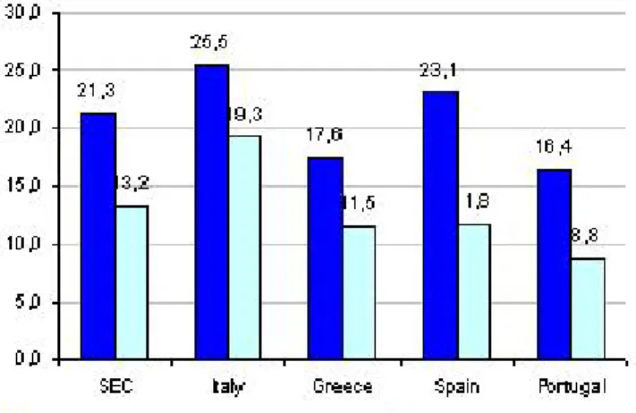
Some descriptive statistics of the sample (tables 6 and 7 appendix B) show that in Italy there is the highest percentage of poor among young people (26%) both before and after they have left parental home.

In each country the youth are mostly male, but looking at the sample of youth who have left home the percentage of women increase strongly in Italy in Spain and Greece, showing that the women are more likely to leave home to form a stable union than men. Portugal and Italy have the lowest rate of youth with tertiary level of education, but in Italy this is compensated by the most of the youth that have the second level of education. Portugal, instead, seems to be the less educated country among the southern European countries (67% of youth have just compulsory school). As we expected the percentage of youth with degree increase if we look at the sample of youth that have left home: 10 point percentage in Greece and only 3 point in Italy and Portugal. This result confirms that the steps in the transition of adulthood are not consequentially but they can overlap.

The first descriptive statistics on the poverty status among youth are shown in the figure and the table below.

home, in other words the percentage of youth considered poor at t (when they still lived at home) and the percentage of youth considered poor at t + 1

(when they left parental home to live with a partner)2_.

In Italy there is the highest rate of youth poverty both before and after the young people have left home. In Spain we can see the biggest gap between the percentage of poor people before and after the departure from home. It is clear that remain at home is a protection against poverty in all Mediterranean countries, in fact, as the graph below shows, the percentage of poor people increase for those who had left home.

Figure 1: Poverty rate before and after leaving parental home (youth aged 19-34)

2_{We end up with a total number of observations for youth outside parental home of}

The transition matrix confirms this result (tab. 1): in Spain there is the highest rate of poor youth that remain poor after they left parental home (50%), and together with Italy, Spain shows also the highest rate of youth not poor in the family of origin but poor as they have left the parental home (respectively 21% and 20%). At this first stage, so we could conclude the Spanish youth are more likely to be at risk of intergenerational transmission of poverty than their same age in the others SEC. On the other hand the transition matrix shows that Greece goes in the opposite direction of the other SEC, only the 26,7% of poor youth remain poor after they had left home

Table 1: Transition matrix of percentage of youth poor

Poverty Status at t + 1 Country Poverty Status at t

Not Poor Poor

Italy Not Poor 78,9 21,1

Poor 56,3 43,7

Greece Not Poor 83,6 16,4

Poor 73,3 26,7

Spain Not Poor 80,4 19,6

Poor 50,0 50,0

Portugal Not Poor 86,0 14,0

Poor 58,3 41,7

All Not Poor 82,0 18,0

5

Model estimates and implications

We estimate the Heckman Probit as described above where in both the selec-tion and the outcome equaselec-tion we control for the same explanatory variables (sex, education, health, family structure, tenure status, quality of neighbour-hood and quality of the relationship outside the family). We estimate the model for each country separately, and pooling all the countries together, in-cluding for countries interactions. We did it because we would like to analyse whether or not the poverty status in the previous family matter or rather it is more a matter of income.

The Wald test of independence of the equations shows that ρ (the correla-tion between the errors terms) is not significant different from zero in all the specifications and in all the countries. This means that the Heckman proce-dure is helpless, the outcome is not different from the outcome obtained by fitting the probit and selection models separately. As first result, therefore, we can argue that in all the countries there is no sample selection bias on the intergenerational transmission of poverty, this bias does not occur even if we pool all the countries together.

So, we provide the main results of the analysis using a probit model to estimate both the probability to be poor in t + 1 and the probability to leave home as part of a couple. We present in the appendix the table of the coefficient for the specification with four dummy variables explaining the economic status in the family of origin as we described in the previous

section. The estimates for the other specifications of income do not provide any additional results.

The economic status of family of origin has a strong impact on the prob-ability to be poor at t + 1 for Italy, Spain and Portugal. In Greece, instead, the economic status in the previous family does not influence the probability to be poor of the youth has left the parental home. In the first specification, the economic status of the family of origin is expressed by a dummy variable that reflect whether or not the family of origin of the youth is poor: being poor in t increase the probability to be poor in t + 1 in all the countries except for Greece.

The second specification of income is the log of income, a continuous explanatory variable that again confirm the stronger correlation in Spain compare to the others.

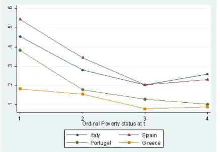
Finally, looking at different dummy for different fraction of Median, for instance, having an income above the 60% of the Median decreases the prob-ability to be poor after leaving home, compare to the reference category of having an income under the 60% of the Median the probability to be poor decrease considerably if the family of origin. The figure 2 confirms that the intergenerational transmission of poverty is stronger in Spain: holding all the explanatory variable at their mean, except the parental income, the predicted probability to be poor at t + 1 is higher in Spain than in the other SEC.

Figure 2: Predicted probability to be poor at t+1 plotting on ordinal poverty measure holding all the explanatory variables at their mean

1)under 60% of Median 2)between 60% and 100% of Median, 3)between 100% and 150% of Median, 4)above 150% of Median

Looking at the individual characteristics (tab. 8 in appendix B) we can state that we do not find a gender effect on the probability to be poor at t + 1 in Italy, Spain and Portugal, however, in Greece, in all the specification considered, being men increases the probability to be poor at t + 1 . We do not find any correlation between the education and the probability to be poor in all the countries, only in Spain and Portugal having a bad health

increases the probability to be poor after leaving home. Pooling all the

countries together we can not find any neighbourhood effect, in fact neither the coefficient of living in a good environment nor having a good relationship with neighbourhood seem to be significant difference from zero.

Looking at the difference within countries we can observe that in Greece, the presence of noise in the neighbourhood of the family of origin seems to decrease the probability to be poor at t + 1. This is not true for all the otthers. Using interaction between the explanatory variables and country dummies, we can confirm the analysis above: there are no big differences in the Southern European countries on the intergenerational transmission of poverty.

Regarding the outcomes equation, the table 2 shows the marginal effects on probability to be poor at t + 1 (holding all the other variables at their means) using different measures of income of the family of origin. Again, the marginal effect of the poverty status at t is stronger in Spain than in the other SEC, and for Greece it is not significant.

In the second specification of income (the log of parental income),in Spain and in Portugal an increment of 1% in the income in the family of origin reduces the probability to be poor in the new family of 12%, again in Greece is not significant.

Regarding the selection equation, the table 8 in the appendix B, provides the estimates for a probit model where the dependent variable is the prob-ability to leave home as a part of a couple. This model is estimated for all the sample of youth aged between 18 and 34 years old.

The results show that there is a strong positive correlation between the income of the family of origin and the probability to leave home. In the table 9 the reference category for the income dummies is having an income

Table 2: Marginal effects on probability to be poor at t + 1 (holding all the other variables to their means) using different measures of income of the family of origin Specifications Country (1) (2) (3) (a) (b) (c ) SEC 0.23 (0.033) -0.1 (0.0138) -0.12 (0.022) -0.18 (0.022) -0.18 (0.024) Italy 0.19 (0.051) -0.09 (0.025) -0.13 (0.042) -0.2 (0.040) -0.15 (0.041) Spain 0.26 (0.069) -0.12 (0.027) -0.13 (0.046) -0.23 (0.043) -0.22 (0.048) Portugal 0.23 (0.076) -0.12 (0.026) -0.11 (0.035) -0.17 (0.042) -0.18 (0.042) Greece 0.09 (0.089) -0.05 (0.035) -0.02 (0.074) -0.09 (0.060) -0.09 (0.071) (1) Poverty status at t (2) Log of income (3) Equivalised income: a)between 60% and

100% of Median, b)between 100% and 150% of Median, c)above 150% of Median

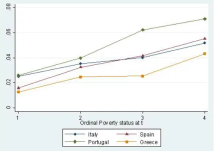
below the 60% of the Median, and we can see that in each country having an income higher than this threshold increase the probability to leave home. The figure 3 confirms the analysis showing an increase in probability to leave home as a couple even if the probability in itself is very low. The Portugal is the country where this probability is higher.

There is a strong gender effect in the selection equation in all the speci-fications considered, we can see that the probability to leave home is higher for female than male, this is strongly significant in all the country.

Figure 3: Predicted probability to leave home at t + 1 plotting on ordinal poverty measure holding all the explanatory variables at their mean

1)under 60% of Median 2)between 60% and 100% of Median, 3)between 100% and 150% of Median, 4)above 150% of Median

In Italy, we find a strong effect of the family type, as also the interactions (tab. 9) show we can not find this effect in the other SEC. The sample is constituted of family with children, they are divided in three category: single, couple and other type of family with children. In Italy the probability to leave home decrease if the youth live in a ‘traditional’ family. In Italy, moreover seems to be important the Social Life that the youth have before to leave home.

If we look at the relationship between the two variables used to identify the sample selection model (i.e. the number of children and the crowding index) we do not find any correlation between them and the probability to leave home except for Italy. The table 3 shows the marginal effects on probability to leave parental home at t + 1 (holding all the other variables at their means) using different measures of income of the family of origin. They are estimated using the probit model. For all the countries we find a negative correlation between the poverty status of the family of origin and the decision of leaving home as part of a couple. The poorer you are in the family of origin the less likely you are to leave home. Here the effect is stronger in Portugal meanwhile in Italy is very low: being poor a t decreases the probability to leave home only of 1.4% compare to the other SEC.

Table 3: Marginal effects on probability to leave home at t + 1 (holding all the other variables to their means) using different measures of income of the family of origin Specifications Country (1) (2) (3) (a) (b) (c ) SEC -0.022 (0.001) 0.013 (0.001) 0.02 (0.003) 0.03 (0.003) 0.04 (0.004) Italy -0.014 (0.002) 0.007 (0.002) 0.01 (0.005) 0.02 (0.005) 0.03 (0.006) Spain -0.027 (0.003) 0.013 (0.002) 0.03 (0.007) 0.04 (0.007) 0.05 (0.008) Portugal -0.031 (0.005) 0.022 (0.004) 0.02 (0.010) 0.06 (0.010) 0.06 (0.011) Greece -0.02 (0.003) 0.013 (0.003) 0.02 (0.009) 0.02 (0.008) 0.04 (0.009) (1) Poverty status at t (2) Log of income (3) Equivalised income: a)between 60% and

6

Conclusion

In southern European countries there is a negative association between parental income and leaving home as part of a couple, in other words the poorer the family of origin is, the less likely is youth to leave home as a couple. The youth stays at home longer but this is not because the risk of poverty is higher than the other age group, in fact we do not find any sample selec-tion bias estimating the Heckman probit where the outcome equaselec-tion is the probability to be poor after leaving home and the selection equation is the probability to leave home as a part of a couple.

The two separate probit show that the economic status of family of origin has a strong impact on the probability to be poor at t + 1 for Italy, Spain and Portugal. We do not find any correlation between parental and children income.

The persistence of poverty seems to be stronger in Spain respect to the other SEC.

References

[1] Aassve A., Iacovou M., Mencarini L., 2005 ‘Youth Poverty in Europe: what do we know?’ ISER w.p. no.2005-2, Colchester, Uk

[2] Aasve A., Davia M., Iacovou M., Mazzuco S., 2005 ‘Leaving home and poverty among youth: a cross European analysis’ EPUNET conference paper 2006, Barcelona, Es

[3] Blanden J., Gibbons, S., 2006, ‘The persistence of poverty across gen-erations’, Joseph Rowntree Foundation, The Policy Press, Bristol, Uk [4] Canto-Sanchez O., Mercader-Prats M., 1999 ‘Poverty among children

and youth in Spain: the role of parents and youth employment status’, Fundacion de Estudios de Economia Aplicada, EEE(ETS) series no. 46, Madrid, Es

[5] Canto-Sanchez O., Mercader-Prats M., ‘Young people leaving home: the impact on povrty in Spain’ in Dynamics of child poverty in industrialised countries edited by B. Bradbury, S. Jenkins and J. Micklewright, Cam-bridge University Press, CamCam-bridge, Uk

[6] Iacovou M., ‘Patterns of family living’ in Iacovou M., Berthoud R., 2004 Social Europe. Living standards and welfare states, Edward Elgar, Chel-tenham, UK

[7] Iacovou M., 2001, ‘Leaving Home in the European Union’, ISER w.p. no.2001-18

[8] Iacovou M., Berthoud R., 2001 ‘Young people’s lives: a map of Europe’ Report ISER, Colchester, Uk

[9] Manacorda, M. Moretti, E., 2005, ‘Why do most Italian men live with

their parents? Intergenarational transfers and household structure’,

Centre for Economic Policy Research, discussion paper no. 5116, Rome, It

[10] Schizzerotto A., Lucchini M. ‘Transitions to adulthood’ in Iacovou M., Berthoud R., 2004 Social Europe. Living standards and welfare states, Edward Elgar, Cheltenham, UK

[11] Smeeding, T.M. and Ross Phillips K., 2002, ‘Cross-National Differences in Employment and Economic Sufficiency’, Annals of the American As-sociation of Political Science, vol. 580, 103-133

[12] Vella, F. 1998, ‘Estimating models with sample selection bias: a survey’, The Journal of Human Resource vol. 33, no. 1 127-169

Appendix A

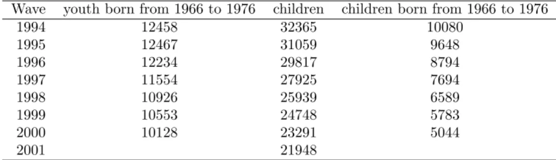
For the analysis of this paper three files wave-specific and one file that cover all the waves have been used. The first group of the ECHP User Data-base files contains the relationship file, the household file, and the personal file. The relationship file is a record of relationship between each pair of person in the same household, the household file is a record for each house-hold with a completed interview, finally the personal file is a record for each person aged 16 year and over with a completed personal interview. In the second group, the UDB contains the country file in which they are recorded the population figures, the purchasing power parities and the exchange rates to convert ECU to EURO. The table 4 shows the sample size in each step to construct the sample of youth at risk to experience the event i.e. leaving parental home in one of the 8 waves.

Table 4: Number of observations in each passages

Wave youth born from 1966 to 1976 children children born from 1966 to 1976

1994 12458 32365 10080 1995 12467 31059 9648 1996 12234 29817 8794 1997 11554 27925 7694 1998 10926 25939 6589 1999 10553 24748 5783 2000 10128 23291 5044 2001 21948

For the first step has been used the personal file to select all the youth in the panel born between 1966-1976 and the personal file has been merged

with household file to get the income variable for all youth in the sample. The construction of the income variable which the analysis related on is described in the second section of this paper. Then from the relationship file (step 2) has been selected all the children in the panel living in the household. Finally in the step three, all the files have been merged to get the final number of observation for the analysis for each wave: i.e. all the children born between 1966 and 1976 and with the income variable and with completed questionnaire.

The last step in the construction of panel is the merge each wave at t with each wave at t + 1 in this way we can get six files with a number of total observations of 45132 individuals. The panel is an unbalanced panel with repeated observations. The follow table shows the distribution by country of whether or not the young peoples have left home in one of the wave. As it is shown there is 11% of attrition in the sample, meanwhile the most of youth born between 1966 and 1976 are still at home in the period considered.

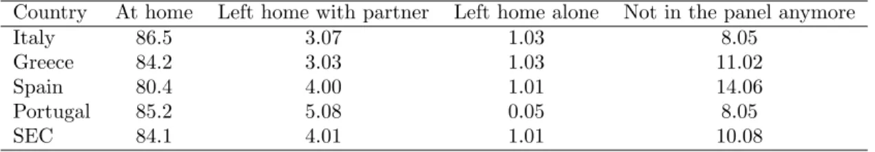
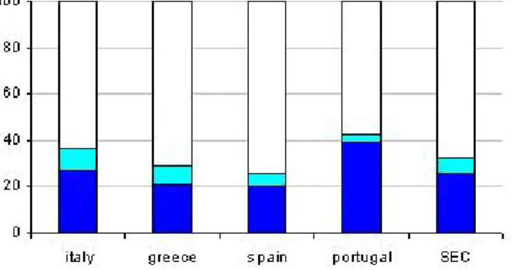
Table 5: Percentage of youth in t + 1 by different outcomes

Country At home Left home with partner Left home alone Not in the panel anymore

Italy 86.5 3.07 1.03 8.05

Greece 84.2 3.03 1.03 11.02

Spain 80.4 4.00 1.01 14.06

Portugal 85.2 5.08 0.05 8.05

SEC 84.1 4.01 1.01 10.08

The figure 4 shows that in Portugal there is the highest percentage of youth who left home to live with a partner. Very few youth have left home alone, this confirm the hypothesis that in SEC the decision to leave home

and form a partnership occur at the same time.

Appendix B

The tables 6 and 7 show the descriptive statistic (mean and standard deviation) for each country and for each variable created at t and t + 1 i.e. before and after the youth has left home. So, in the first table the sample for which the descriptive statistics are calculated is all the youth at risk to leave home in one wave of the panel, they are aged between 18 and 33 years old. In the second table the sample is constitute on all the youth who had left home in one wave in the sample to live with a partner, they are aged 19-34. Each table show the variable at individual and household level, of course the variables at household level in the first table shown the characteristics of the family of origin of the youth.

The tables 8 and 9 show the estimate for one specification of the model for each country and pooling all the countries together including some in-teraction. We control for interactions with countries and all the explanatory variable but we report only the significative ones. The references category is always the interaction with Italy.

However, the reference category for the income dummies is the equivalised income below the 60% of the Median of the income, for the health status is fair health, for the level of completed education is the compulsory education. For the tenure status is the accommodation for free, for the structure of the family is the single without children and finally for the country is Italy.

Table 6: Descriptive statistics of youth (aged 18-34) in the family of origin at t

Variable at t Italy Spain Greece Portugal All

Mean SD Mean SD Mean SD Mean SD Mean SD

Individual characteristics Male 0.55 0.5 0.55 0.5 0.57 0.5 0.59 0.49 0.56 0.5 Age 24.4 3.4 24.1 3.3 24.6 3.4 24.0 3.4 24.3 3.4 Poverty Status 0.26 0.44 0.25 0.43 0.22 0.42 0.17 0.37 0.23 0.42 EqInc¡60%Me 0.26 0.44 0.25 0.43 0.22 0.42 0.17 0.37 0.23 0.42 60%Me¡EqInc¡100%Me 0.25 0.43 0.23 0.42 0.21 0.41 0.24 0.43 0.24 0.43 100%Me¡EqInc¡150%Me 0.26 0.44 0.26 0.44 0.27 0.44 0.31 0.46 0.27 0.44 EqInc¿150%Me 0.23 0.42 0.26 0.44 0.3 0.46 0.28 0.45 0.26 0.44 Equivalized income 9704 6631 8344 6451 8256 6364 7517 5363 8652 6362 Bad health 0.02 0.13 0.02 0.13 0.02 0.13 0.05 0.21 0.02 0.15 Fair health 0.11 0.31 0.08 0.27 0.02 0.14 0.15 0.36 0.09 0.29 Good health 0.88 0.33 0.91 0.29 0.97 0.18 0.81 0.4 0.89 0.32 Tertiary ed.(ISCED 5-6) 0.05 0.22 0.24 0.43 0.2 0.4 0.04 0.21 0.13 0.34 Secondary ed.(ISCED 3-4) 0.58 0.49 0.38 0.49 0.53 0.5 0.29 0.45 0.46 0.5 Compulsory ed.(ISCED 0-2) 0.37 0.48 0.38 0.49 0.27 0.44 0.67 0.47 0.41 0.49

Good social life 0.91 0.28 0.96 0.2 0.93 0.26 0.8 0.4 0.91 0.29

Good relat. with neighb. 0.72 0.45 0.85 0.35 0.94 0.23 0.84 0.37 0.82 0.39 Household characteristics

Single with children 0.11 0.31 0.13 0.33 0.12 0.33 0.13 0.34 0.12 0.33 Couple with children 0.78 0.42 0.68 0.47 0.66 0.47 0.59 0.49 0.69 0.46 Other family with children 0.11 0.31 0.2 0.4 0.22 0.41 0.28 0.45 0.18 0.39

Owner 0.82 0.39 0.88 0.33 0.86 0.35 0.75 0.43 0.83 0.38 Tenant 0.16 0.36 0.09 0.29 0.12 0.33 0.17 0.37 0.13 0.34 Free accommodation 0.03 0.16 0.03 0.18 0.02 0.13 0.08 0.28 0.04 0.19 Presence in neighbourhood Crime 0.19 0.39 0.22 0.41 0.06 0.24 0.13 0.33 0.17 0.37 Pollution 0.19 0.39 0.16 0.37 0.17 0.38 0.13 0.33 0.17 0.37 Noise 0.32 0.47 0.35 0.48 0.23 0.42 0.17 0.37 0.29 0.45 House crowded 0.62 0.04 0.61 0.05 0.62 0.05 0.61 0.06 0.62 0.05 Number of children 2.41 1.18 2.83 1.49 2.36 1.25 2.82 1.69 2.61 1.41 Number of observations 16488 13698 7359 9007 46552

Table 7: Descriptive statistics of youth (aged 18-34) in their own family at t+1

Variable at t+1 Italy Spain Greece Portugal All

Mean SD Mean SD Mean SD Mean SD Mean SD

Individual characteristics Male 0.45 0.5 0.46 0.5 0.45 0.5 0.55 0.5 0.48 0.5 Age 27.2 2.8 26.8 2.7 26.1 3.0 25.7 2.9 26.5 2.9 Poverty Status 0.25 0.44 0.23 0.42 0.18 0.38 0.16 0.37 0.21 0.41 Bad health 0.01 0.09 0.01 0.09 0 0 0.02 0.12 0.01 0.1 Fair health 0.14 0.35 0.08 0.27 0.03 0.16 0.16 0.37 0.11 0.32 Good health 0.85 0.36 0.91 0.29 0.97 0.16 0.83 0.38 0.88 0.33 Tertiary ed.(ISCED 5-6) 0.08 0.27 0.32 0.47 0.3 0.46 0.07 0.26 0.18 0.38 Secondary ed.(ISCED 3-4) 0.52 0.5 0.24 0.43 0.43 0.5 0.2 0.4 0.34 0.47 Compulsory ed.(ISCED 0-2) 0.4 0.49 0.44 0.5 0.27 0.44 0.73 0.44 0.48 0.5 Good social life 0.89 0.32 0.96 0.19 0.97 0.16 0.89 0.31 0.92 0.27 Good relat. with neighb. 0.8 0.4 0.81 0.39 0.95 0.21 0.79 0.41 0.82 0.38

Household characteristics

Couple with children 0.22 0.42 0.13 0.34 0.22 0.42 0.29 0.45 0.22 0.41 Couple without children 0.73 0.44 0.82 0.38 0.73 0.44 0.63 0.48 0.73 0.45 Other type of couple 0.05 0.21 0.05 0.22 0.05 0.22 0.08 0.28 0.06 0.23

Owner 0.52 0.5 0.64 0.48 0.53 0.5 0.53 0.5 0.56 0.5 Tenant 0.3 0.46 0.21 0.4 0.36 0.48 0.22 0.41 0.26 0.44 Free accommodation 0.18 0.39 0.15 0.36 0.12 0.32 0.25 0.43 0.18 0.39 Presence in neighborhood Crime 0.11 0.31 0.15 0.36 0.05 0.23 0.07 0.25 0.1 0.3 Pollution 0.12 0.33 0.1 0.31 0.12 0.33 0.09 0.29 0.11 0.31 Noise 0.31 0.46 0.26 0.44 0.19 0.39 0.16 0.37 0.24 0.43 Number of observations 597 555 259 528 1939

Table 8: Probit model on the probability to be poor at t + 1

Probability to be poor at t + 1 Italy Spain Greece Portugal SEC Interaction Eqinc between 60%and100%Median -0.47** -0.51* -0.11 -0.62** -0.50*** -0.43*** Eqinc between 100%and150%Median -0.72*** -0.94*** -0.51 -0.83*** -0.77*** -0.62*** Eqinc above 150%Median -0.53** -0.84*** -0.44 -0.97*** -0.72*** -0.59***

Male 0.05 -0.11 0.55** 0.09 0.08 -0.07**

Tertiary education at t + 1 0.01 -0.09 0.1 -0.33 -0.1 -0.20***

Secondary education at t + 1 -0.19 0.04 -0.04 0.05 -0.08 -0.16***

Couple with children at t + 1 0.14 0.08 0.15 0.18 0.15 -0.03

Other type of couple at t + 1 0.25 0.85** 0.06 0.16 0.29* 0.01

Bad health at t + 1 0.43 1.42* 1.02 0.91**

Good health at t + 1 -0.08 -0.04 0.24 -0.18 -0.1

Owner at t -0.29 -0.08 5.66*** -0.32 -0.28 -0.16***

Tenant at t -0.37 -0.57 5.93*** -0.31 -0.38* -0.10*

Good social life at t -0.31 0.54 0.43 -0.27 -0.12 -0.01

member club or organization at t 0.16 -0.03 0.77 0.07 0.1

noise problems at t -0.12 -0.1 -0.55* 0.14 -0.1 -0.06*

trafic/industry pollution at t -0.08 -0.11 0.46 0.19 0.00 -0.06

crime/vandalism in area at t 0.09 0.29 -0.19 0.48 0.19 -0.08*

Good social relationship at t -0.16 -0.23 0.23 -0.13 -0.13 -0.04

Spain 0.02 -0.01

Greece -0.21 -0.32

Portugal -0.33*** -0.82***

Constant 0.47 -0.35 -8.53 -1.29 0.04 -0.54***

Table 9: Probit model on the probability to leave home

Probability to leave home at t + 1 Italy Spain Greece Portugal SEC Interaction Eqinc between 60%and100%Median 0.15** 0.31*** 0.27** 0.19* 0.21*** 0.18*** Eqinc between 100%and150%Median 0.21*** 0.42*** 0.28** 0.40*** 0.32*** 0.12* Eqinc above 150%Median 0.33*** 0.55*** 0.52*** 0.47*** 0.44*** 0.32***

Male -0.18*** -0.19*** -0.26*** -0.10* -0.17*** -0.18***

Tertiary education at t -0.02 -0.05 0.06 0.00 0.00 -0.02

Secondary education at t -0.10* -0.31*** -0.20** -0.24*** -0.21*** -0.10* Single with children at t -0.60*** -0.16 -0.16 -0.20* -0.28*** -0.48*** Couple with children at t -0.33*** -0.16** 0.00 -0.08 -0.16*** -0.34***

Bad health at t -0.23 -0.27 -0.18 -0.42** -0.35*** -0.23

Good health at t -0.01 -0.1 0.41 0.02 -0.01 0.00

Owner at t 0.05 0.21 0.3 -0.07 0.03 0.03

Tenant at t 0.02 0.21 0.32 -0.04 0.03 0.03

Good social life -0.13* -0.03 0.02 0.16** 0.02 -0.12

member club or organization at t 0.07 0.17*** 0.24* -0.06 0.09**

noise problems at t -0.03 0.00 0.02 0.00 -0.01 -0.03

trafic/industry pollution at t 0.06 0.01 0.12 0.04 0.04 0.06

crime/vandalism in area at t -0.07 -0.04 -0.08 0.07 -0.04 -0.07

Good social relationship at t 0.11* 0.01 0.00 0.05 0.06* 0.06*

Number of children at t 0.10*** -0.02 0.00 0.01 0.03 0.04 House crowded at t 3.09*** -0.32 0.98 -0.32 0.82 0.75 Spain -0.04 0.1 Greece -0.11** -0.79 Portugal 0.11*** -0.52* (Spain)*SecondEd at t -0.22*** (Portugal)*SecondEd at t -0.14* (Greece)*singwchil at t 0.34* (Spain)*singwchil at t 0.29** (Portugal)*singwchil at t 0.23* (Greece)*couplewch at t 0.35** (Spain)*couplewch at t 0.18* (Portugal)*couplewch at t 0.25** (Portugal)*socLife at t 0.27** Constant -3.73*** -1.84** -3.83*** -1.75** -2.50*** -1.66*** legend: ∗p < 0.05; ∗ ∗ p < 0.01; ∗ ∗ ∗p < 0.001