Coverage in wireless sensor networks: models and algorithms

UNIVERSITY OF SALERNO

DEPARTMENT OF COMPUTER SCIENCE PhD in COMPUTER SCIENCE

CYCLE XIII

PhD THESIS IN COMPUTER SCIENCE

Coverage in

Wireless Sensor Networks:

Models and Algorithms

Candidate Ciriaco D’Ambrosio

Tutor Co-Tutor

Prof. Raffaele Cerulli Dr. Francesco Carrabs

Coordinator Prof. Giuseppe Persiano

Acknowledgements

During my PhD I had the great pleasure to work with wonderful and professional people and I wish to express my gratitude to everybody for the great research experience that they have granted me. I would like to thank Professor Raffaele Cerulli, my wise tutor, for his help, his many precious suggestions and his constant encouragement dur-ing my PhD He was for me a real guide. I would like also to express my great gratitude to my exceptional co-tutor, Francesco Carrabs, for his collaboration, his patience and for teaching me to always pursue my goals. He was for me a precious point of reference. I am also very grateful to Andrea Raiconi for his guidance, his patience and his fundamental contributions to this research work. He demonstrated great dedication to help me in this research. I am also very thankful to Monica Gentili for her collaboration and her professional sugges-tions. Finally, I thank all my family and my dear friend Arcangelo Castiglione for their support and constant presence, and last but not least, I want to thank Sara with whom I shared every moment of my PhD.

Abstract

Due to technological advances which enabled their deployment in rel-evant and diverse scenarios, Wireless Sensor Networks (WSNs) have been object of intense study in the last few years. Possible applica-tion contexts include environmental monitoring, traffic control, pa-tient monitoring in healthcare and intrusion detection, among others (see, for example, [4], [16], [37]). The general structure of a WSN is composed of several hardware devices (sensors) deployed over a given region of interest. Each sensor can collect information or mea-sure physical quantities for a subregion of the space around it (its sensing area), and more in particular for specific points of interest (target points or simply targets) within this area. The targets located in the sensing area of a given sensor s are covered by s. Individual sensors are usually powered by batteries which make it possible to keep them functional for a limited time interval, with obvious con-straints related to cost and weight factors. Using a network of such devices in a dynamic and coordinated fashion makes it possible to overcome the limitations in terms of range extension and battery du-ration which characterize each individual sensor, enabling elaborate monitoring of large regions of interest. Extending the amount of time over which such monitoring activity can be carried out represents a very relevant issue. This problem, generally known as Maximum Lifetime Problem (MLP), has been widely approached in the litera-ture by proposing methods to determine: i) several subsets of sensors each one able to provide coverage for the target points and ii) the activation time of these subsets so that the battery constraints are satisfied. It should be noted that while sensors could be considered

as belonging to different states during their usage in the intended ap-plication (such as receiving, transmitting, or idle) in this context two essential states can be identified. That is, each sensor may currently be active (i.e. used in the current cover, and consuming its battery) or not. Activating a cover refers therefore to switching all its sen-sors to the active state, while switching off all the other ones. This research thesis shows a detailed overview about the wireless sensor networks, about their applications but mainly about typical coverage issues in this field. In particular, this work focuses on the issue of maximizing the amount of time over which a set of points of interest (target points), located in a given area, can be monitored by means of such wireless sensor networks. More in detail, in this research work we addressed the maximum lifetime problem on wireless sensor net-works considering the classical problem in which all targets have to be covered (classical MLP) and a problem variant in which a portion of them can be neglected at all times (α-MLP) in order to increase the overall network lifetime. We propose an Column Generation ap-proach embedding an efficient genetic algorithm aimed at producing new covers. The obtained algorithm is shown to be very effective and efficient outperforming the previous algorithms proposed in the liter-ature for the same problems. In this research work we also introduce two variants of MLP problem with heterogeneous sensors. Indeed, wireless sensor networks can be composed of several different types of sensor devices, which are able to monitor different aspects of the re-gion of interest including temperature, light, chemical contaminants, among others. Given such sensor heterogeneity, different sensor types can be organized to work in a coordinated fashion in many relevant application contexts. Therefore in this work, we faced the problem of maximizing the amount of time during which such a network can remain operational while assuring globally a minimum coverage for all the different sensor types. We considered also some global regular-ity conditions in order to assure that each type of sensor provides an adequate coverage to each target. For both these problem variants we

developed another hybrid approach, which is again based on a column generation algorithm whose subproblem is either solved heuristically by means of an appropriate genetic algorithm or optimally by means of ILP formulation. In our computational tests the proposed genetic algorithm is shown to be able to meaningfully speed up the global procedure, enabling the resolution of large-scale instances within rea-sonable computational times. To the best of our knowledge, these two problem variants has not been previously studied in the literature.

Contents

Contents vi

List of Figures ix

Nomenclature xii

1 Introduction 1

1.1 Wireless Sensor Network: Motivation . . . 1

1.2 Contributions of this thesis . . . 3

1.3 Organization of Dissertation . . . 4

1.4 Reading this document . . . 5

2 Coverage Optimization in Wireless Sensor Networks 6 2.1 Introduction . . . 6

2.2 Wireless Sensor Networks Overview . . . 8

2.2.1 Sensor Coverage Models . . . 10

2.2.2 Coverage Problems and Design Issues . . . 13

2.2.2.1 Coverage Problem Types . . . 13

2.2.2.2 Design Issues . . . 14

2.3 Network Lifetime and Coverage Optimization . . . 20

2.3.1 Covers Scheduling on WSN . . . 20

2.3.2 Common Scenario and Problem Definition . . . 22

3 Maximum Lifetime Problem: Modeling and Algorithms 25 3.1 Modeling the problem . . . 25

3.2 Column Generation . . . 28 vi

CONTENTS

3.2.1 Restricted Master Problem Formulation . . . 29

3.2.2 Modeling the Separation Problem . . . 30

3.2.3 Working Scheme . . . 34

3.2.4 How to solve the separation problem . . . 37

3.3 Genetic Algorithms . . . 37

3.3.1 Generational Genetic Algorithms and Steady State Algo-rithms . . . 40

4 A Hybrid Exact Approach for Maximizing Lifetime in Sensor Networks with Complete and Partial Coverage Constraints 44 4.1 Introduction . . . 44

4.2 Problems Definition and Mathematical Formulation . . . 46

4.3 Column Generation Approaches for α-MLP and MLP . . . 50

4.3.1 Heuristic approaches to speed-up the Column Generation Approach . . . 51

4.4 A Genetic Algorithm to Solve the Subproblem [SP] . . . 52

4.4.1 Chromosome Representation and Fitness Function . . . 54

4.4.2 Crossover . . . 55

4.4.3 Mutation . . . 57

4.4.4 Fixing and Redundancy Operators . . . 57

4.4.5 Building the Initial Population . . . 58

4.4.6 GA Overall Structure . . . 59

4.5 Computational Results . . . 61

5 The Maximum Lifetime Problem of Sensor Networks with Mul-tiple Families 69 5.1 Introduction . . . 69

5.2 Notation and Problems Definition . . . 73

5.2.1 Modeling Hardware Differences . . . 75

5.2.2 MLMFP, MLMFP-R and cover redundancy . . . 76

5.3 Column Generation Approach . . . 76

5.4 Genetic Algorithm . . . 80

5.4.1 Chromosome representation and fitness function . . . 81 vii

CONTENTS

5.4.2 GA overall structure . . . 83

5.4.3 Tournament selection . . . 84

5.4.4 Crossover . . . 85

5.4.5 Mutation . . . 86

5.4.6 Fixing and redundancy operators . . . 87

5.4.7 Building the initial population . . . 88

5.5 Computational Results . . . 89

5.5.1 Description of instances and test scenarios . . . 89

5.5.2 Parameter setting and CG initialization . . . 91

5.5.3 Test and Results . . . 92

6 General Conclusions 103

Appendix A 105

Appendix B 108

References 118

List of Figures

2.1 Components of a Sensor Node . . . 11

2.2 Coverage Types: (a) area coverage - (b) points coverage . . . 14

2.3 Transformation . . . 15

2.4 Barrier Coverage Example . . . 16

2.5 Layered Wireless Sensor Network . . . 18

2.6 Covers Examples . . . 23

2.7 Sensor scheduling in the optimal solution for the instance in figure 2.6 . . . 24 3.1 Examples of covers . . . 27 3.2 CG Diagram . . . 36 3.3 GA Diagram . . . 43 4.1 Example Network . . . 47 4.2 Hybrid Scheme . . . 53

4.3 The chromosome representation. . . 54

4.4 The crossover operator. . . 56

5.1 Sample network. A-B: Feasible non-redundant covers C1, C2. C: Complete network and feasible redundant cover C3. . . 77

5.2 Chromosome Structure . . . 81

5.3 Gene structure . . . 85

5.4 Crossover . . . 86

5.5 Computational time of CG+GA for both MLMFP and MLMFP-R with _{|F | = 4 . . . .} 97

LIST OF FIGURES

5.6 Lifetime for both MLMFP and MLMFP-R with _{|F | = 4 . . . .} 99

B.1 Computational time of CG+GA for both MLMFP and MLMFP-R with _{|F | = 2 . . . 109} B.2 Computational time of CG+GA for both MLMFP and MLMFP-R

with _{|F | = 6 . . . 111} B.3 Lifetime for both MLMFP and MLMFP-R with _{|F | = 2 . . . 114} B.4 Lifetime for both MLMFP and MLMFP-R with _{|F | = 6 . . . 115}

Nomenclature

List of Abbreviations

α-M LP Maximum Network Lifetime Problem with partial coverage constraint

CG Column Generation

CG + GA Exact Approach for M LM F P CGonly Pure Exact Approach for M LM F P Exact Deschinkel Exact Approach for M LP

GA Genetic Algorithm

GCG Genetic Column Generation, exact approach for α-M LP

GR Gentili and Raiconi Approach for α-M LP

Heur Deschinkel Heuristic Approach for M LP

ILP Integer Linear Programming

M EM S Micro-Electro-Mechanical Systems M ixed Deschinkel Mixed Approach for M LP

M LM F P Maximum Lifetime with Multiple Families Problem

M LM F P _{− R Regular Maximum Lifetime with Multiple Families Problem} M LP Maximum Network Lifetime Problem

LIST OF FIGURES

P Master Problem

QoS Quality of Service

RP Restricted Master Problem

SP Separation Problem

W SN Wireless Sensor Network

Chapter 1

Introduction

1.1

Wireless Sensor Network: Motivation

Wireless sensors networks (WSNs) were presented as one of the most promising technology that would change the world [88]. In the last ten years a lot of re-search have been conducted in this field and nowadays there is a growing interest in this technology. One could mention, for instance, the popularity of the recent technology concept known as “The Internet of Things” [7] [81], that is based on networks of smart objects which are globally connected to the Internet and include modular sensors as well as other technologies to collect and process infor-mation on the environment around them. There is therefore a current increasing economic interest for all smarter technologies and in particular for Wireless Sen-sor Networks, which justifies expectations of growing investments, as mentioned in some recent market research reports to industries, such as “Semiconductor Wireless Sensor Networks Markets at $ 2.7 billion in 2013 are forecast to reach $ 12 billion Worldwide by 2020” [87]. In today’s world where people are con-stantly surrounded by smartphones, smart applications and smart objects, the sensor networks are constantly more and more widely used. Their main objective is to reach a better knowledge of the events occurring in the environment around people and in which people live. Sensor networks are an essential tool to bet-ter study the impact that natural and man-made phenomena may have on the environment including, the effects on climate, pollution, safety and many other

1. INTRODUCTION

aspects. Such a technology is also a useful tool for scientists interested in studying some events and physics phenomena which still remain difficult to fully compre-hend and predict. One could think of natural disasters such as earthquake, flood and so on. In these scenarios such networks are very useful, since they are able to constantly monitor the environment in unattended manner. In such scenarios the sensors may be deployed and controlled by flying drones, enabling secure remote control of a scenario without direct risks for the humans. Thanks to this scien-tific and economic interest, today Wireless Sensor Networks can be considered a mature technology even if there are some technology constraints, mainly related to the energy resources, that encouraged the research world to study and find new solutions. In these last years, the battery technology evolution has been less impressive than in others, such as micro electronic systems and even if there are new system that allow sensors to obtain a certain quantity of energy from the en-vironment [104] [109], it remains a critical resource and should be used carefully. The constrained energy resource of a sensor is therefore one of the main issues in order to prolong as much as possible the sensor lifetime. Indeed, if a sensor depletes its energy resources, it generally becomes useless because it is difficult to supply additional energy to such sensors. These limits severely affect the avail-ability of the network services. Prolonging the network operational time is a basic requirement in the design of a wireless network in terms of architecture, hardware and algorithms for the management of the sensors. For this reason, this line of research has been object of intense studies, which led to the design of heuristic and approximate algorithms, among others, based on distributed or centralized approaches. The time for which a network is able to guarantee the monitoring activities is typically called Network Lifetime. Besides energy limitations, the networks are also subject to others environment constraints, such as coverage or connectivity constraints. The mostly used approaches for energy efficiency can be divided into two main families, known as power-aware scheduling and duty scheduling of the sensors activities. A power-aware configuration algorithm aims to identify network configurations able to minimize the energy consumption as-sociated with the network operations/tasks. They can be generally adopted in structured network scenarios with low-density sensors as discussed [1] [11] [94]. The second approach principally aims to assign a working status to a subset of

1. Introduction

sensors able to satisfy the network coverage requirements for a proper amount of time. Only a subset of sensors is active at any given time, avoiding to waste the energy of unnecessary nodes. This technique is widely used for high density network scenarios, for instance in adverse scenarios with hostile environments in which a precise placement of the sensors is not possible, nor is possible to supply additional energy resources [17] [30] [90]. Even if the approaches of the first type such as routing schemes and power aware nodes configurations try to address the problem of extending the network lifetime as well, they suffer of other problems such as the well known “Hot-spot Problem” as reported in [1]. The approaches of the second type are generally preferable because they provide comprehensive solutions that are not affected by this type of issue. Generally, in unstructured networks with high density of sensors, there is a large number of possible subsets of sensors able to satisfy the coverage constraints, named feasible covers or simply covers. Therefore the maximum lifetime can be found by searching these covers and activating them, one at a time, for proper amounts of time. This approach is known as “duty scheduling”, and plans to design the activities of the sensors in the network to ensure a monitoring for as long as possible [22] [30] [29] [54] [84] [112]. Starting from these basic motivations, in this thesis, we study the cur-rent literature about the Wireless Sensor Networks to design and propose exact efficient approaches for the Maximum Network Lifetime Problem under different coverage constraints. Motivated by heterogeneity of modern networks such as the Internet of Things, we investigated two variants of the basic problem in the case of heterogeneous sensor networks.

1.2

Contributions of this thesis

This thesis consists of an in-depth study on wireless sensor network on their ap-plications and on typical coverage issues in this field. Particular focus is dedicated to the problem of maximizing the amount of time over which a set of points of interest (target points) located in a given geographic region can be monitored by means of a wireless sensor network. The problem is well known in the literature as the Maximum Network Lifetime Problem (MLP). We focused mainly on an algorithmic aspect of the problem rather than on a technology aspect. It is

exam-1. INTRODUCTION

ined the column generation technique and how to apply it to the mathematical formulation MLP and three problem variants. It is showed how to embed in the column generation a genetic meta-heuristic aimed at solving the separation prob-lem, that is shown to be very efficient for all the considered problem variants. The problems studied in this work include the α-MLP problem, a variant in which a subset of sensors can be left uncovered. However, since α-MLP is a generalization of MLP, our algorithms can be used to solve the classical problem as well. As will be shown in the discussion of our computational tests our algorithm is proven to be highly efficient with respect to the previous algorithms available in the litera-ture. The other two studied MLP variants are related to heterogeneous sensors. Today wireless sensor networks are generally composed of several different types of sensor devices, which are able to monitor different aspects of the region of interest (including sound, vibrations, chemical contaminants, among others) and may be deployed together in a heterogeneous network. In this work, we address also the problem of maximizing the amount of time during which such a network can remain operational while assuring globally a minimum coverage for all the different sensor types. The second problem variant in this context also consid-ers some global regularity conditions, in order to guarantee a fair coverage for each sensor type to each target. In our computational tests the proposed resolu-tion approach is shown to be very effective, enabling the resoluresolu-tion of large-scale instances within reasonable computational times.

1.3

Organization of Dissertation

This work is organized as follows:

• Chapter 2 introduces some general concepts on wireless sensor networks and their functionalities. This chapter also presents the main sensor coverage models, some coverage issues and the related design choices. Then are shown some aspects of coverage optimization and the main literature results related to this field are discussed.

• Chapter 3 introduces a mathematical formulation of the MLP. Then it shows how to apply the column generation technique to solve the problem. It is

1. Introduction

shown how to hybridize such an exact approach with heuristics. Finally, the chapter presents an overview on genetic algorithms.

• Chapter 4 presents the hybrid exact approach for the MLP and α-MLP problems. It describes all the building blocks of specialized genetic meta-heuristic that we designed to solve the separation problem of the Column Generation approach.

• Chapter 5 illutrates our research work on two novel variants of the MLP problem defined on heterogeneous sensor networks. Starting from the de-scription of the two problems, we present the related mathematical formu-lations, the hybrid exact approaches we developed to solve both of them and the results of our computational tests.

• Chapter 6 includes our conclusions on these works and a summary of the obtained results. It shows also some future research directions about our considered field of research.

1.4

Reading this document

This manuscript is structured in such a way that the six chapters can be read independently. This first chapter briefly introduces the reader to this work and its structure. The readers interested in the research content may directly refer to Chapter 4 and Chapter 5. Chapter 4 refers to homogeneous wireless sensor network with global or partial coverage requirements, and, it corresponds to a work submitted to Journal of Network and Computer Applications. Chapter 5 refers to heterogeneous wireless sensor networks, and it corresponds to a work published on Computers and Operations Research. Chapter 2 and Chapter 3 show the essential background for the research content, therefore the readers interested to the theory and the techniques adopted may start by reading Chapter 2 for an general introduction to the Wireless Sensor Networks and Chapter 3 for a detailed description of the column generation and its application to the problem as well as an introduction on genetic algorithms.

Chapter 2

Coverage Optimization in

Wireless Sensor Networks

2.1

Introduction

Wireless Sensor Networks nowadays are one of the most advanced systems able to collect and process information from the environment. Wireless Sensor Networks perform monitoring through the installation of a significant number of sensors (or sensor nodes) that detect, store and communicate local information that will be eventually used to make global decisions on the environment. Unlike traditional computer systems that process data and information produced by men, WSNs deal with information coming from the environment in which they are installed [44] [21]. This growing “symbiosis” between the world and this innovative nology has attracted and stimulated the interest of many researchers. The tech-nological improvements, in recent years, in the field of micro-electro-mechanical systems (MEMS), digital electronics and in the field of wireless communications, among others, allowed the wireless sensor networks to achieve, today, the state of very mature technology. The miniaturization of computing and sensing de-vices encouraged the development of a type of network with a very wide range of applications. Early research in this field was dictated by military applications such as acoustic surveillance and target detection. Today there are systems for 360-degree monitoring, systems for the monitoring and protection of civil

infras-2. Introduction

tructures such as bridges, tunnels, meeting areas, power grids, water networks and pipelines. In particular sensor networks have already been used for pollution control, flooding, for the control of health, and in agriculture for the control of the use of fertilizers, pesticides as well as for the control of natural water usage in order to improve the crop’s health and production. Another interesting field of application is the traffic control, some applications include the installation of sensors along the main streets and on cars in order to control and improve traffic flow and avoid jams. These and many other applications from general monitor-ing, to healthcare, and even more generally to national security are described and surveyed in [3] [107] [4] [36] [16] [37] and many other works. Since when the first sensor network prototypes have been proposed, such as Smart Dust [66], the research on wireless sensor networks has raised many optimization problems due to both the natural development requirements of sensor networks and the needs of developing increasingly large and efficient networks; recall for instance the IrisNet (Internet-scale Resource-Intensive Sensor Network Services) project at Intel Research, an ideal framework for a worldwide heterogeneous sensor web [55]. An important class of problems is known as Coverage Problems. According to the application of the network the concept of coverage can be defined through different points of view. Generally given a set of targets of interest and a set of coverage constraints, the main goal of the coverage problems is to have each target of interest under monitoring with respect to the coverage constraints. The concept of coverage expresses how well a physical space is monitored by a sensor network [22] and its evaluation expresses the quality of service (QoS)[78] offered by the network. There are different formulations of the coverage problems related to different aspects of the network such as the type of covered object (area, tar-get), the type of sensor placement (random or deterministic) and based on many other properties. For example, one of the most important sensor/network char-acteristics is the energy consumption that strongly influences the time interval for which the network is able to satisfy the application for which it was designed, i.e. the network lifetime. Indeed it is one of the most critical aspects of the WSN applications and one of the most studied properties. There are different applica-tion dependent definiapplica-tions in the literature. One of the first definiapplica-tions considers the lifetime as the time interval between when the network starts to operate and

2. WIRELESS SENSOR NETWORKS OVERVIEW

the first node fails [95]. This definition, as others, doesn’t take in consideration any particular characteristic of the coverage. Today there are various definitions based on the coverage, on the node availability, and others characteristics, all definition can be reviewed in [42]. In this thesis, the network lifetime is the time interval for which the network is able to meet the specific coverage requests of the application. It is the most general definition which is suited to coverage problems. If a network cannot guarantee the desired coverage request then it is considered as not being operational. It is well known that the energy efficiency is one of the issues that generally arise in all kinds of wireless sensor networks and that affects the network lifetime. The networks are composed of sensors of limited size and weight. These structural constraints severely affect the availabil-ity of services offered by the WSN. Since sensors generally have limited energy resources and limited communication features. If a sensor depletes its energy resources, it becomes useless since it is difficult to supply additional energy to it. For these reasons, prolonging the life time of a sensor network, as much as possible, by finding patterns of energy preservation is one of the main objectives to be met in order to achieve energy efficiency. This chapter aims to introduce general information about sensor networks and the basic technical details for the formulation of coverage problems with special emphasis on the design of energy efficient networks. In particular, we will focus on the problem of covering targets with known positions and energy constraints.

2.2

Wireless Sensor Networks Overview

The applications listed in the previous introduction (Sec 2.1) are only a subset of all possible uses of WSN. The underlying technology for sensor networks may vary for architectures and functionalities, but there are some common charac-teristics and features. The main common characteristic is the integration with the environment. A WSN is integrated in the phenomenon or environment for which it was developed. The sensors register the phenomenon in which they are immersed, they monitor the target points in surrounding space, they commu-nicate with each others, transmitting detailed informations on the environment under monitoring. The analysis of the environment, through the capture of light,

2. Wireless Sensor Networks Overview

temperature, sound, vibrations and so on, can reveal the nature of the physical space. The word “sensing” includes all the measurement activities and control of status changes of the phenomenon or of the environment under monitoring. Measurement, preliminary elaboration and reporting of the sensed information are in short the main objectives of the small devices called sensors. In this work we will use the term sensor and sensor node interchangeably. However to be pre-cise, a sensor node is the sensing unit which includes with tools such as battery, antenna, possible actuators among others, while sensor refers only to the actual hardware device which is able to perceive the status changes of the phenomenon. Another well known term used to refer to a sensor is transducer, i.e. a system able to transform physical quantities into electrical signals. For more details on the structure of a sensor node, see Figure 2.1. As shown in the figure, its main four components are a sensing unit, a processing unit, a transceiver unit and a power unit. Obviously, the sensing unit can vary depending on what is to be monitored. In addition the sensor may be equipped, depending on the applica-tion, with additional components such as tracking systems, eventual generators of additional energy [109] and also actuators. The analog signals, perceived from the environment by the ”sensor” subcomponent of the sensing unit, are converted to digital, by the “ADC” unit. Once converted to digital, the signals are passed to the “Processing Unit”. The processing unit, typically coupled to a “Storage Unit”, manages the procedures and scheduling activities required to efficiently collaborate with the other nodes in the network. The “Power Unit” is among the most important ones and as previously said is sometimes supported by spe-cific hardware (“Power Generator” in the Figure 2.1) to obtain energy from the environment, see for example [109]. Some sensor nodes use location mechanisms through which the sensor identifies its position in space and/or actuators that allow to complete more complex sensing tasks. The sensors, as reported in Fig-ure 2.1, can be equipped with a transceiver for the network connection through RF or optical drives. All these components are subject to tight dimensional con-straints. Indeed, in some cases a sensor node is contained in a box [64] of a cubic centimeter [83]. They are also subject to many other general constraints such as low power consumption, operational capacities in high density condition, low pro-duction costs, absolute autonomous control and adaptation to the environment.

2. WIRELESS SENSOR NETWORKS OVERVIEW

Given such constraints it is straightforward to understand that the lifetime of a WSN strongly depends on the battery duration of the sensors that compose it. Generally sensors can be either static or mobile, however in this work we focus on static nodes. A static (or fixed) node does not change its position, and represents the most common case. Conversely a mobile sensor may be equipped with mo-bility systems [33] or be positioned on moving devices such as robots or vehicles [34] [73].

2.2.1

Sensor Coverage Models

Sensors nodes may have many different characteristics from both a physical and a theoretical point of view. Taking into account the various aspects described in the introduction it is straightforward to note that different sensing models may be adopted. The sensing models can be based on the environment, on the design choices and on the application requirements and they express a measure of the sensing ability and its quality, evaluating the relation among the environment, the sensors and the targets. As reported in [77] and remarked later in [111] and other works, the sensor nodes typically have two intrinsic common characteristics: (1) the quality of sensing diminishes as distance increases (2) the sensing ability improves as the sensing time increases. Typically sensing models can be expressed in function of the Euclidean Distance among target points and sensors. We generally consider the concept of coverage, as in the majority of the works cited in this thesis, in the two dimensional space. Given a point z in the space under monitoring and the set of sensors S = _{s1, s2, ..., sn}, spread over the area of

interest, the Euclidean Distance between a generic sensor s and point z can be expressed as follows: d(s, z) = q (sx− zx) 2 + (sy− zy) 2 (2.1) where obviously s and z are individuated by their Cartesian coordinates (sx, sy) for s and (zx, zy) for z. As reported in [102] we could also consider a

2. Wireless Sensor Networks Overview Processing  Unit             Processor   Storage   Sensing  Unit       Sensor   ADC   T r a n s c e i v e r   Power Unit Power  Generator   Loca5on   Finding   System   Actuator       Power Unit

2. WIRELESS SENSOR NETWORKS OVERVIEW

Euclidean Distance of each space point with respect to the whole set of sensors, can be considered a function f that for each space point expresses a coverage measure through this formula f:(d(S, z), ϕ(S, z)) _{→ <}+ _{where S is the set of all}

the sensors in the network. Also in [102] it is reported that by means of simple modifications this evaluation can be used in three-dimensional contexts. Gener-ally the sensing models that consider a boolean evaluation of the coverage, i.e. 0 or 1, are called Boolean or Binary Coverage Models. Models that consider non-negative coverage measures are called General Coverage Models. Models that do not consider the angle as function input are called Omnidirectional Coverage Models, as opposed to Directional Coverage Models. For a more detailed and extensive review of the sensing models the reader can refer to [102]. In our works we considered the most studied and simplified sensing model, the binary disk coverage model that considers as coverage function the following formulation:

f (d(s, z)) =    1, if d(s, z)_{≤ R}sense 0, otherwise (2.2)

where we can recall that d(s, z) is the Euclidean Distance between a generic sensor s and z a generic target point that we want to monitor. Rsense is called

sensing range or sensing radius, it is defined by the sensor technology and it defines the sensing area of the sensor centered on the device. It does not consider an angle as input therefore it is an omnidirectional coverage model. All the space point within the sensing area of a given sensor are defined as being covered by it. Generally for each space point we can consider the sum of the function values evaluated for all sensors that defines whether a space point is covered or not by the network, as follows:

f (S, z) =

n

X

i=1

fi(d(si, z)) (2.3)

If this f (S, z) = K then the sensor can be defined as K-Covered (i.e. there exist K sensors that cover z). There are also other models such as Boolean Sector

2. Wireless Sensor Networks Overview

Coverage Models, Attenuated Disk Coverage Models, Detection Coverage Models and others [102] that model different coverage types.

2.2.2

Coverage Problems and Design Issues

Besides the previously mentioned elements there are other differentiations that generally complicate the network design as well as other aspects. Different cover-age problems arise from the possible design choices. Covercover-age Problems constitute a research topic of crucial relevance for the design of communication protocols and algorithms for the efficient management of the sensors. Coverage problems may differ on the basis of the object of sensing (area or discrete points), deployment type (random or deterministic), sensor mobility capabilities, or network structure (simple or composite), among other factors. In the course of this chapter, we will give a general overview on the different coverage types and their related design issues, and will finally focus on the problem definition on which our research is based and that, as we will see, generalizes all formulations.

2.2.2.1 Coverage Problem Types

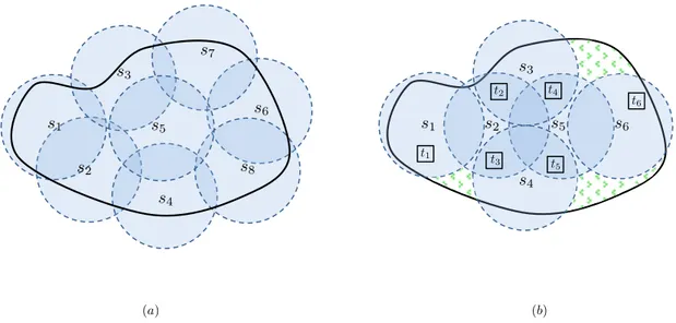
Generally the coverage problems can belong to three main coverage families, that is: (i) area coverage problems, (ii) point or target coverage problems and (iii) barrier coverage problems [25]. In the former the main objective is to monitor a whole area of interest. In the second family the objective is to monitor only a set of discrete points which may be specific objectives within the environment. Figure 2.2-a shows an irregular area covered completely by the sensor network. Figure 2.2-b shows the same area and a set of targets which are covered by the network. In the second case, the targets coverage request can leave some zones of the area uncovered. However in the literature it is well know that an area coverage instance can be easily transformed into a target coverage one [98] and we can refer to both indifferently. The polynomial time transformation is based on the concept of “field”, i.e. a subset of the area which is covered by the same set of sensors. We achieve the transformation by replacing each field with a target point. Figure 2.3 gives an idea of such simple transformation. Therefore, for simplicity we generally refer to target coverage problems.

2. WIRELESS SENSOR NETWORKS OVERVIEW s6 s5 s4 s3 s2 s1 s7 s8 s3 (a) (b) t1 t6 t2 t5 t3 t4 s6 s5 s4 s2 s1

Figure 2.2: Coverage Types: (a) area coverage - (b) points coverage

In barrier coverage problems the main objective is to build intrusion barriers for the detection of moving objects that can cross over or enter the area of interest. Let us consider Figure 2.4. This figure reports an illustration of barrier coverage. In Figure 2.4-a we can see an area that we want to monitor, a barrier coverage made of sensors along the boundaries of the area and an intrusion movement from the upper side of the area towards the lower side. In this case we can observe a real barrier coverage because the area can not be crossed from a one side to another without intersecting the sensing disk of the sensors. In Figure 2.4-b we can see a movement that can cross the region of interest without intersecting the sensing disk of the sensors. Therefore in this second case the network cannot provide a barrier coverage. It is straightforward to note that the barrier coverage doesn’t require to coverage the whole area of interest. More details on intrusion barriers and penetration paths can be found in [102] [68] [69] [76].

2.2.2.2 Design Issues

Given the sensing models and the three main families of coverage problems, we can now analyze the various design issues or design choices as reported in [102] [21], that may characterize a coverage problem:

2. Wireless Sensor Networks Overview

s

s

s

s

(a) Area Coverage Instance (b) Fields Identification

(c) Target Coverage Instance

2. WIRELESS SENSOR NETWORKS OVERVIEW (a) (b) Intrusion Movement Intrusion Movement t6 t1 t2 t5 t3 t4 s6 s5 s4 s3 s2 s1 s7 t6 t1 t2 t5 t3 t4 s6 s5 s4 s3 s2 s1 s7

Figure 2.4: Barrier Coverage Example

• Coverage Type: as previously mentioned and described in Section 2.2.2.1 we can have area coverage, target coverage and barrier coverage problems. • Deployment Type: there exist two deployment types that strongly affect the network topology: deterministic (or structured) and random (or un-structured) [107]. Deterministic installations are considered in the case of small and easily accessible area and the positioning is designed ad-hoc for the surrounding environment. Sensor placement can be designed to use as few sensors as possible in order to reduce both the management and main-tenance costs. In the case of large and/or difficult to access area, random positioning could be preferable or mandatory. In the unstructured case, the network is composed of a large number of sensors which are positioned randomly and after the installation, the network is left unattended to per-form its monitoring activities. In this type of network is it more difficult to address the issues of a typical communication network, such as how to manage the connectivity or possible failures. The choice of the deployment type depends on the environment.

2. Wireless Sensor Networks Overview

percentage of the area the sensor network needs to cover in order to satisfy the coverage requirements. Generally we refer to complete coverage when the network covers the whole area or the whole set of targets. We refer to partial coverage when the network needs to cover only a subset of points to satisfy the coverage requirements. We can say that if the network covers 70 targets out of 100, its coverage ratio is 70%.

• Coverage Degree: each target can be monitored by one or more than one sensor at each time. When each node of the sensor network is covered by at least k sensors the networks has a k-coverage degree. Typically this aspect is relevant when the network needs to guarantee a certain level of coverage robustness since a sensor network that satisfies a such requirement, can tolerate up to k_{− 1 damages or faults for each sensor node.}

• Sensors type: technology offers different sensors and there are cases in which monitoring is performed by sensors with different characteristics. The choice is often application dependent, some application requires that all sensor nodes in the network are equal or with the same characteristics, while others require different sensor nodes types (see for example the problems faced in Chapter 5 of this work).

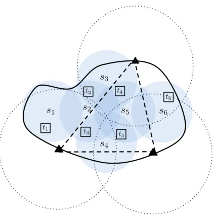
• Sensors Mobility: as previously mentioned sensors may be static or mobile. • Network Type: simple or mixed. The type is simple when a network is composed only of sensors that send information to a single collection node called sink, either in a centralized manner or a distributed one. The type is mixed or layered, if the network is composed of simple sensors (also with different technical and sensing characteristics) and a subset of more powerful nodes that act as collection nodes. In Figure 2.5 it is showed a dual layer sensor network in which a set of simple sensors (grey circles) can sense and process information about the environment, and a second layer of more powerful nodes (dotted circles) collect the information in order to efficiently manage the sensing tasks.

• Collection Nodes Mobility: some works assume that the collection nodes are static, other works assume that the sinks are mobile. Recent technologies

2. WIRELESS SENSOR NETWORKS OVERVIEW

s

s

s

s

s

s

2. Wireless Sensor Networks Overview

allow for instance the integration of robots which play the role of collection nodes in sensor networks [13] [70] [99] [39].

• Events Type: a network can monitors either atomic or composite events. As reported in [21] a fire event can be better monitored if there are more combined information as temperature, smoke, humidity. In this case an heterogeneous network has to satisfy specific coverage requirements for each atomic event [27].

• Coverage Breach: a target point or an area is defined breached when it is not covered by a sensor node. Some applications require a target or area monitoring that minimize the time for which the targets/areas remain uncovered. Sometimes the applications can require to minimize the total number of breached target points.

• Activity Scheduling: refers to the ability of the network to change the state of a sensor node. Generally it refers to the capacity of the sensor network to switch in a sleep energy-saving state the redundant active sensors. The main objective of this activity is typically to save energy in order to prolong the time for which the network can operate. This activity is governed by algorithms that belong to two main categories, namely centralized or dis-tributed. Many centralized and distributed algorithms have been developed in this research field. Generally the distributed algorithms allow each node to decide about its state basing the process on the distributed information in the network. This process generally reduces the communication energy but intensifies the processing energy consumption. The centralized algo-rithms, on the other hand, leave each node to only send its sensed data to a central collector node that also makes global decisions about the working states of all sensors. This type of algorithms highly reduce the processing energy consumption. More details about the Activity Scheduling can be found in the next Sections.

• Network Connectivity: even if this requirement is typically related to the network layer it is also considered in the design of specialized algorithms to define certain cross layer operations. Two nodes can be defined as connected

2. NETWORK LIFETIME AND COVERAGE OPTIMIZATION

if they are able to send and receive data directly between them. In other cases two nodes can be defined as connected if there are some others nodes between them that act as relays. Generally a network can be defined as connected if each couple of sensor nodes is connected and the data of each node can be sent to the collector node as well as to other nodes. In such a case sensors have a communication range in addition to the sensing range. Generally the communication range is larger than the sensing range. All these design choices have some unifying requirements for the efficient func-tionality of the wireless sensor network. As already discussed a crucial one is the energy efficiency of the network in order to improve the “network lifetime”.

2.3

Network Lifetime and Coverage

Optimiza-tion

Network lifetime was originally defined as the amount of time until the first operational failure of a sensor occurs [42]. Definitions such as the previous one are incomplete because, especially in the case of unstructured networks with an high density of sensors, the network can be operational even if one of the sensors has depleted all its energy or has been damaged. These observations suggest different definitions, mainly linked to the coverage as in our research works (see Chapter 4 and 5), or related to the availability of nodes in the network or to the connectivity. In [42] the reader can find a full list of the main definitions. In this thesis, the network lifetime is the time interval for which the network is able to meet the specific coverage requests of the application. The absence of specific assumptions about the network, allows to adapt the definition to a wide range of different design choices.

2.3.1

Covers Scheduling on WSN

It is straightforward to understand that optimize the usage of constrained energy resource of a sensor is the main issue to be taken in consideration in order to prolong as much as possible the network lifetime. In the literature there are

2. Network Lifetime and Coverage Optimization

different approach to address energy efficient coverage to extend the network lifetime. The first approach, on which are based our research works, is to define a schedule plan of the sensor activity that leaves some sensors in active state while the others are into a sleep state that does not consume energy. A second approach consists of designing an efficient coverage deployment plan, but is not always practical. A third approach is based on adjusting the sensing range in order to save energy. The first approach requires to identify covers, i.e. subsets of sensors, able to achieve the coverage requirements of the network [22] [23] [54] [59] [96]. This type of approach can be further divided in two main subcategories. A first one based on disjoint set of sensors as in [98] [24] and a second one based on non-disjoint set of sensor as in [22]. In the case of disjoint subsets, the covers do not share sensors, that is, the subsets have empty intersections. The second proposed approach allow the covers to share sensors among them. It has been proved that this approach can achieve greater lifetimes than the first one. In the case of disjoint subsets each cover is activated for all battery duration one at time while all sensors that do not belong to it are either in sleep mode or have been previously used. The authors in [98] proposed an heuristic algorithm to find as many covers as possible in order to extend the network lifetime. The duty scheduling was extensively investigated by researchers. Today there are many approaches that follow this idea while considering different characteristic of the network [31] [60] [65] [93] [54] [27]. It is important to note that the disjoint covers approach doesn’t aim to maximize directly the lifetime, but rather tries to find the maximum number of possible covers. In the second case, in addition to the coverage constraints, covers can be activated even for very small amounts of time. The non-disjoint covers idea was investigated only in recent years and it is receiving more and more attention. Modeling lifetime problems on this idea has led to more realistic formulations. This approach aims at directly maximizing the lifetime by finding the optimal covers schedule and the related activation times, while satisfying all battery and network coverage constraints. The algorithms that follow this approach typically face hard optimization problems as in the case of the problems that we face in Chapters 4 and 5.

2. NETWORK LIFETIME AND COVERAGE OPTIMIZATION

2.3.2

Common Scenario and Problem Definition

The scenario addressed in our work takes into account unstructured networks with random deployment and a high density of sensors. The sensors, with limited energy resources, are typically scattered in the region of interest and perform a monitoring activity on target points disposed within the area. The information gathered by the sensors is distributed among them, and we assume that such information will be collected and delivered to a central node at the end of the monitoring phase. The central node is also assumed to coordinate the activity of the sensors. Generally the sensor operational states are identified TRANSMIT, RECEIVE, IDLE or SLEEP. Taking into account the previous works in this field [22] [26] it is well known that the power usage of most units, such as the seismic sensor WINS Rockwell, is similar for the transmit state, the receive state and for the idle state while the sleep state requires a much lower, not negligible amount of energy. Therefore as in other works [54] [31], we assume for simplicity that two main operating states exist, called ACTIVE and SLEEP, which identify, generally, the cases in which a sensor is consuming battery for or not. Under these assumptions, we can observe that an accurate use of covers can improve considerably the network lifetime. Consider the example in Figure 2.6. In the example we have three targets T =_{t1, t2, t3} and four sensors S={s1, s2, s3, s4}.

The sensor s1 covers the targets t1 and t2. The sensor s2 covers the targets t1

and t3. The sensor s3 covers t2 and t3 and the sensor s4 covers all targets. For

all sensors we consider an energy resource normalized to 1 unit of time, i.e. each sensor can be in the active state for 1 unit of time before depleting all its energy. We recall that we want to cover all targets. If we active all sensors at the same time the overall network lifetime is equal to 1 since there are not other sensors available for monitoring. If we consider subsets of sensor, e.g. covers C1={s1, s2},

C2={s1, s3}, C3={s2, s3}, C4={s4}, as in Figure 2.6-b-c-d-e, we can improve the

network lifetime. Each one of these covers meets the coverage request, i.e. each subset of sensors covers all targets. Therefore we can design a strategy that activates first cover C1={s1, s2} for 0.5 unit of time, then cover C2={s1, s3} again

for 0.5 units then C3={s2, s3} for other 0.5 units and finally C4={s4} for 1 unit.

2. Network Lifetime and Coverage Optimization t1 _t 2 t3 s1 s2 s3 s4 t1 _t 2 t3 s1 s2 t1 t2 t3 s1 s3 t1 _t 2 t3 s2 s3 t1 _t 2 t3 s4 (a) (b) (c) (d) (e)

Figure 2.6: Covers Examples

2.5 times higher than the one obtained using the first, trivial strategy.

As shown, this approach can lead to considerable extensions of the network lifetime. This is particularly true on dense networks where targets are redun-dantly covered by sensors whose ranges present many overlaps. In this instances, indeed, a large number of feasible covers can exist and can be used to identify the optimal solution. This problem has been widely studied in recent years (refer to the literature overviews in chapters 4 and 5) and is usually known as Maximum Wireless Sensor Network Lifetime Problem (MLP). It has been shown to be Np-Complete by reduction from 3-SAT problem in [22]. There are also some related variants that consider different design choices such as the ones that we face in our research work described in Chapters 4 and 5.

2. NETWORK LIFETIME AND COVERAGE OPTIMIZATION

s

s

s

s

s

s

s

Figure 2.7: Sensor scheduling in the optimal solution for the instance in figure 2.6

Chapter 3

Maximum Lifetime Problem:

Modeling and Algorithms

3.1

Modeling the problem

As extensively detailed in previous Chapter 2, Wireless Sensor Networks are com-posed of a huge number of sensors scattered over a geographic area that we want to monitor. Each sensor device has limited sensing and limited computational resources. Each of them senses the surrounding space around it defined by its sensing range. All the sensors perform a complex sensing task about the environ-ment around them. A sensor can gather information about all its surrounding area or only about specific targets inside its sensing area. From now on we will refer only to target coverage problems for the motivations given in Section 2.2.2.1. Given the energy battery constraints, one of the main issue is to prolong as much as possible the network lifetime, i.e. the amount of time for which the network is able to guarantee the coverage constraints about the subject under monitoring. As reported in Section 2.3 the network lifetime can be extended by individuating covers and activating them, one at time, for a suitable amount time. In this chapter we formally define the Maximum Lifetime Problem (MLP) on Wireless Sensor Network and we describe the basic concepts of the column generation technique and the genetic algorithms that we will use to address this problem. Let N = (S, T ) be a wireless sensor network, where S =_{s1, . . . , sm} is the set of

3. MODELING

sensors and T =_{t1, . . . tn} is the set of targets. Each sensor has a given sensing

range defined by its technical characteristics and each sensor is powered by a battery that can keep it in an active state for a limited amount of time. Here, for simplicity, we assume that each sensor has the same characteristics, i.e. same sensing range and same battery lifetime normalized to 1. We consider a omnidi-rectional binary sensing disk model (see Section 2.2.1). Therefore for each target tk ∈ T and sensor si ∈ S, we define a binary parameter δki equal to 1 if tk is

located inside the sensing area of si (target tkis covered by the sensor si), 0

other-wise. Let C be a subset of sensors (C_{⊆ S). We formally define C to be a feasible} cover, for the network N , if all targets of the network are covered by at least one sensor, i.e. P

i∈Cδkixi ≥ 1 ∀k = 1, ..., n. The Maximum Lifetime Problem

con-sists in finding a collection of pairs (Cj, wj), where Cj ⊆ S is a feasible cover and

wj ≥ 0 is the amount of time for which the sensors belonging to Cj are kept in an

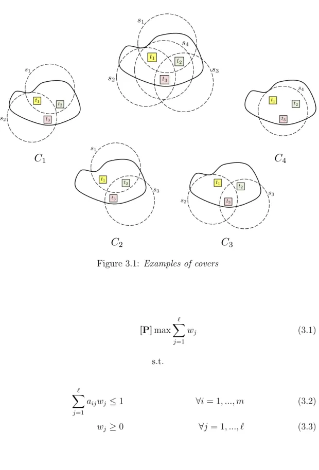
active state (i.e. activation time), such that the sum of the all activation times is maximized and each sensor is used globally for an amount of time that does not exceed its normalized energy resource. In the figure 3.1 we can see a very simple sensor network composed of 4 sensors and 3 targets. Possible examples of covers that can be activated to monitor all targets are: C1 = {s1, s2}, C2 = {s1, s3},

C3 ={s2, s3}, C4 ={s4}. Therefore, assuming to be able to compute the whole

set of feasible covers C1, . . . , C` in advance, MLP could then be represented using

the Linear Programming formulation [P], where wj are the variables associated

to the columns of the matrix, _{∀j, with j = 1, ..., l. The variables indicate the} activation time of each cover. As seen in Section 2.3.2 we consider two particular relevant operating states, called ACTIVE and SLEEP, which identify the cases where a sensor is consuming battery for sensing or not. Then the binary param-eter aij indicates if a sensor si is active in a covers Cj, i.e. aij = 1 if si ∈ Cj,

0 otherwise. We can note that each column a_j is a representation of a cover, therefore from now on we use the terms “cover” and “column” indifferently:

3. Modeling t1 _t 2 t3 s1 s2 s3 s4 t1 _t 2 t3 s1 s2 t1 _t 2 t3 s1 s3 t1 _t 2 t3 s2 s3 t1 _t 2 t3 s4

C

C

C

C

Figure 3.1: Examples of covers

[P] max ` X j=1 wj (3.1) s.t. ` X j=1 aijwj ≤ 1 ∀i = 1, ..., m (3.2) wj ≥ 0 ∀j = 1, ..., ` (3.3)

3. COLUMN GENERATION

The objective function (3.1) maximizes the network lifetime i.e. the sum of the activation times wj, while constraints (3.2) require that each sensor cannot be

ac-tivated for more than its battery resource. In real world scenarios, the number of sensors is often very large with respect to the number of targets. Consequently, the number of covers (columns of the model) is too large (i.e. potentially ex-ponential) for a direct application of the simplex method, both in terms of time (needed to check the optimality condition on the exponential non-basic variables) and space (needed to build the constraints matrix). A proper approach to the resolution of this problem is the well known Column Generation (CG) algorithm, a technique alternative to the Simplex algorithm, that starts by solving the model [P] with a small subset of columns and then introduces additional columns until the optimal solution of [P] is found. The column generation algorithm differs from the Simplex algorithm in how it performs the optimality test of the current basic solution and in how the new variable to eventually enter the basis is cho-sen. Indeed, in the case of the Column Generations these steps are performed by modeling and solving an auxiliary optimization problem.

3.2

Column Generation

As reported in [75] and in [80], the first idea of Column Generation was pre-sented in a work of Ford & Fulkerson (1958) [46]. This work suggests for the first time to deal with the variables of a problem in implicit manner. They con-sider a multi-commodity maximum flow problem and their idea was to begin by solving optimally a master LP formulation that just contains few columns (ex-treme flows in the work) for each commodity. Then they used an optimal dual solution to price out the columns not yet examined by means of the solution of a shortest path problem, for each commodity. Later, Dantzig & Wolfe (1960) [35] inspired by the work of Ford & Fulkerson [46], generalized the idea to obtain an algorithm for solving linear programming problems individuating a set of master constraints and a set of separation problem constraints, known as Dantzig-Wolfe Decomposition, as also reported in [80]. Later in the two seminal works, Gilmore and Gomory (1961-1963)[56] [57] implemented the technique to solve a problem that involve integer variables, the Cutting Stock Problem. However, the first

oc-3. Column Generation

currence of the column generation naming appeared in 1969 with a paper titled “A column generation algorithm for a ship scheduling problem” [6].

3.2.1

Restricted Master Problem Formulation

Given the mathematical model [P], let R _{⊆ {1, ..., `} be a subset of the indexes of} all possible columns. Through the R columns, we build the [RP] model, named Restricted Master Problem, as follows:

[RP] maxX j∈R wj (3.4) s.t. X j∈R aijwj ≤ 1 ∀i = 1, ..., m (3.5) wj ≥ 0 ∀j ∈ R (3.6)

The coefficients aij, with i ∈ {1, .., m} and j ∈ R, form the matrix AR, i.e.

the matrix obtained by considering only the columns of the original matrix A with index belonging to the subset R. Therefore, the problem [RP] consists of just the variables of [P] associated to the column of AR. Assuming that the R

set is not too large, this restricted formulation can be directly solved by means of the Simplex algorithm. Let w_Rbe the optimal solution of [RP] that from now on we denote as the incumbent solution. Let B_{⊆ {1, ..., `} be the set of the basic</sub> columns, N <sub>⊆ {1, ..., `} the set of the non basic columns, N}0 _{⊆ R − B the set} of non basic columns related to the restricted formulation and b the righ-hand-side column vector. It is easy to see that (w_R, 0_{N −N}0) is a feasible solution for

the original formulation [P]. In this situation there are two conditions that may occur:

• The optimal solution for [RP] is also optimal for [P]. Therefore the master incumbent solution is globally optimal and the column generation procedure stops and returns the incumbent solution.

3. COLUMN GENERATION

• The optimal solution for [RP] is not optimal for [P]. It means that there exists a non-basic variable wj with j ∈ N, with zj − cj < 0, that can

improve the value of the objective function. If the existence of this variable wj is proven, we have to construct the related column aj that has to be

introduced in the matrix AR. Once inserted the variable and the column

in the restricted formulation, the column generation algorithm repeats the whole process.

A proper application of the method requires to face the following issues: 1. How do we find a variable wj having a negative reduced cost among the

exponential variables in N ?

2. Even if we find the variable wj, how do we build the column aj of the

coefficient matrix AR?

3. How do we identify the initial set of columns R?

4. How do we update the set R once the new column to be included is found? 5. How is degeneracy dealt with?

Now we will shortly address each of the above mentioned issues. For the issues 1 and 2, the column generation tries to identify the variable wj and the column

aj, through the resolution of a new optimization problem known as Separation

Problem (or SubProblem) (SP). The separation problem is constructed in an ad-hoc manner depending on the master problem and often it corresponds to well known optimization problems for which efficient algorithms have already been proposed. Since the resolution of the RP is easy, the key point to obtain an efficient column generation algorithm is the ability to efficiently solve the subproblem [SP].

3.2.2

Modeling the Separation Problem

Now we see how to model the separation problem for the classical Maximum Lifetime Problem. Let w∗_R be the optimal solution of the restricted problem

3. Column Generation

[RP]. The matrix composed only of the columns of the variables belonging to the base will be indicated with the form AB. Instead, the matrix corresponding

to the restricted problem will be indicated with the form AR. The columns of

the matrix corresponding to non-basic variables of the restricted problem are indicated in the form AR−B. We denote by AN all the columns not yet generated

joined to the columns in AR−B. Given the initial set of columns R, some of

them will correspond to basic variables, while the remaining N0 will correspond to non-basic variables. Then we can write:

w∗_R= " w_B w_R−B # = " A−1_B b 0_R−B # (3.7) ⇓ w =    w_B w_R−B w_{N −R−B}   =    A−1_B b 0_R−B 0_{N −R−B}   = " A−1_B b 0_N # (3.8)

Taking into account the optimality conditions expressed through the reduced cost values we can state that a current solution is globally optimal if and only if the reduced cost values corresponding to all the non-basic AN columns are

positive, i.e. zj − cj ≥ 0 ∀j ∈ N. Considering the size of the problem it is clear

that it is not possible to evaluate these coefficients in an enumerated manner. The idea of the column generation is based on the search for the smallest reduced cost value evaluating the following objective function that will be the objective of our separation problem:

min

j∈N zj − cj (3.9)

If the value of the minimum reduced cost, corresponding to the objective function (3.9), evaluated on the incumbent solution, is non negative then the optimality conditions for problem [P] are met and therefore there are not non-basic variables that can improve the incumbent solution. Otherwise there exists a column that, once added to the restricted problem RP, may improve it. In this

3. COLUMN GENERATION

case, the column corresponding to the optimal solution of the separation problem will be added to the matrix AR. We observe that:

min j∈N zj − cj (3.10) ⇓ min j∈N c T BA −1 B aj− cj (3.11) ⇓ min j∈N π T_a j− cj (3.12) ⇓ min j∈N m X i=1 aijπi− cj (3.13) ⇓ min j∈N m X i=1 aijπi− 1 (3.14)

By applying the above shown substitutions to objective function (3.10) we can build the formulation of the objective function of the separation problem which is specific for the the Maximum Lifetime Problem. As we know from the theory of linear programming, zj = cTBA

−1

B aj then substituting in (3.10) we get the formula

(3.11). We observe that cT

BA

−1

B corresponds to the simplex multipliers that appear

in the evaluation of the reduced cost values, in other words these values are the dual prices and correspond to the vector πT_{. Substituting in (3.11), we get (3.12).}

By explicating (3.12), we get (3.13), where a_j is the j-th column of the coefficient matrix. Finally we note that the coefficients cost cj of [P] are all equal to 1,

and then we obtain (3.14). It should be noted that in (3.14), each aij value

corresponds to the i-th entry of the new entering column aj that we want to find,

and therefore are the variables of our separation problem. Then, we rewrite the new objective function as follows:

3. Column Generation min m X i=1 xiπi− 1 (3.15)

The variable xi indicates whether the i− th sensor is turned on or off in the

cover which is represented by the new column built by the separation problem. The vector x must be a feasible cover of [P], i.e. its active sensors have to cover all the targets. To this end, we build the following subproblem [SP] in which the constraints impose to satisfy this covering condition.

[SP] min m X i=1 πixi (3.16) s.t. m X i=1 δkixi ≥ 1 ∀k = 1, ..., n (3.17) xi ∈ {0, 1} ∀i = 1, ..., m (3.18)

The objective function (3.16) minimizes the sum of the dual prices of the sen-sors chosen to be part of the newly produced cover. If the optimal solution of this formulation is greater than or equal to 1, then the incumbent solution is guar-anteed to be optimal for the original problem, otherwise the new cover is added to the master problem. The constraints (3.17) define a feasible coverage, that is, every target must be covered by at least one sensor in the current cover. It is straightforward to note that the [SP] formulation corresponds to a specialization of the Set Covering problem, a well known Np-Hard problem.

3. COLUMN GENERATION

3.2.3

Working Scheme

Now we focus our attention on the working scheme of the column generation al-gorithm. Given the linear programming formulation [P], the column generation technique starts by considering the restricted master problem, and solving it to optimality. The optimal solution of the restricted master problem is feasible for the original problem [P], however there is no guarantee regarding global opti-mality since most of its columns have been discarded. The column generation then considers the specific separation problem which either produces an attrac-tive cover to add to the restricted master problem for a new column generation iteration, or certifies that the incumbent solution is optimal. We recall that an attractive cover is a feasible cover corresponding to a non-basic variable with neg-ative reduced cost, which could therefore improve the incumbent solution. The column generation procedure iterates until the above presented optimality con-dition is met. Therefore, this exact approach allows to implicitly discard most of the variables that will be non-basic in the optimal solution. The subsequent algorithm and the diagram 3.2 summarize the working scheme of the column gen-eration approach:

INPUT: Maximum Lifetime Problem Instance 1. Define the initial set of columns R:

The choice of the columns has to guarantee the feasibility for the main problem P.

2. Costruct the RP formulation with the column belonging to R: max_{cT

RwR: ARwR≤ 1, wR≥ 0}.

3. Solve the RP formulation:

Let w∗_R be the optimal solution of the RP problem. 4. Construct and solve the separation problem:

If the optimal solution of the separation problem is _{≥ 1 then the solution} (w∗_R, 0_{N −N}0) is the optimal solution also for [P] and the algorithm stops.

Otherwise the column computed by the separation problem SP is added to the RP formulation and then we return to the step 3.

3. Column Generation

We can now answer to the question 3 of the section 3.2.1 that is: 3) how do we identify the initial set of columns R? The initial choice of the set R of columns has to guarantee the feasibility for the restricted master problem. The general method is to use an heuristic approach to compute any feasible solution of size R for the current problem that we have to solve. Given such heuristic solution, the set R will be composed by columns of the matrix A related to the heuristic solution. A simple example of heuristic solution could be the follow: for each target choose a sensor that covers it and activate it. We don’t care about how many targets a selected sensor covers, as long as we respect the target coverage constraints. This is a simple way to construct a cover. The process may be iterated to produce the desired R set. Another important question is linked to the update of the set R of columns, i.e. 4) how do we update the set R? In literature there exist variants of the column generation approach based on the method used to update the set R at each iteration:

1. the set R can be composed of the basic columns deriving from the last [RP] solution and of the new column that enters the basis. At each iteration the column generated by the separation problem can be added to the set R and the exiting one is deleted.

2. iteration by iteration a new column is added to the set R without deleting previous ones.

3. columns of R which did not enter the basis for a large number of iterations without re-entering are deleted from it.

Indeed, there are cases in which even if the separation problem individuates a new attractive entering variable the objective function doesn’t change its value. This is a situation that slows down the convergence of the algorithm. Generally in case of degeneracy we can apply anti-cycling rules and perturbation rules on the restricted problem. More details about the applicability of the approach can be found in [12] [41] [56] [57] [75] [80].