MUSE integral-field spectroscopy towards the Frontier Fields cluster Abell S1063: II. Properties of low luminosity Lyman α emitters at z > 3

DOI:10.1051/0004-6361/201629055 c ESO 2017

Astronomy

&

Astrophysics

MUSE integral-field spectroscopy towards the Frontier Fields

cluster Abell S1063

II. Properties of low luminosity Lyman

α

emitters at z

>

3

W. Karman

1

, K. I. Caputi

1

, G. B. Caminha

2

, M. Gronke

3

, C. Grillo

4, 5

, I. Balestra

6, 7

, P. Rosati

2

, E. Vanzella

8

, D. Coe

9

,

M. Dijkstra

3

, A. M. Koekemoer

9

, D. McLeod

10

, A. Mercurio

11

, and M. Nonino

7

1 _{Kapteyn Astronomical Institute, University of Groningen, Postbus 800, 9700 AV Groningen, The Netherlands}

e-mail: karman@astro.rug.nl

2 _{Dipartimento di Fisica e Scienze della Terra, Università degli Studi di Ferrara, via Saragat 1, 44122 Ferrara, Italy} 3 _{Institute of Theoretical Astrophysics, University of Oslo, Postboks 1029 Blindern, 0315 Oslo, Norway}

4 _{Dark Cosmology Centre, Niels Bohr Institute, University of Copenhagen, Juliane Maries Vej 30, 2100 Copenhagen, Denmark} 5 _{Dipartimento di Fisica, Università degli Studi di Milano, via Celoria 16, 20133 Milano, Italy}

6 _{University Observatory Munich, Scheinerstrasse 1, 81679 Munich, Germany} 7 _{INAF–Osservatorio Astronomico di Trieste, via G. B. Tiepolo 11, 34143 Trieste, Italy} 8 _{INAF–Bologna Astronomical Observatory, via Ranzani 1, 40127 Bologna, Italy} 9 _{Space Telescope Science Institute, 3700 San Martin Drive, Baltimore, MD 21208, USA}

10 _{SUPA, Institute for Astronomy, University of Edinburgh, Royal Observatory, Edinburgh EH9 3HJ, UK} 11 _{INAF–Osservatorio Astronomico di Capodimonte, via Moiariello 16, 80131 Napoli, Italy}

Received 3 June 2016/ Accepted 23 August 2016

ABSTRACT

In spite of their conjectured importance for the Epoch of Reionization, the properties of low-mass galaxies are currently still very much under debate. In this article, we study the stellar and gaseous properties of faint, low-mass galaxies at z > 3. We observed the Frontier Fields cluster Abell S1063 with MUSE over a 2 arcmin2_{field, and combined integral-field spectroscopy with gravitational}

lensing to perform a blind search for intrinsically faint Lyα emitters (LAEs). We determined in total the redshift of 172 galaxies of which 14 are lensed LAEs at z= 3–6.1. We increased the number of spectroscopically-confirmed multiple-image families from 6 to 17 and updated our gravitational-lensing model accordingly. The lensing-corrected Lyα luminosities are with LLyα . 1041.5erg/s among

the lowest for spectroscopically confirmed LAEs at any redshift. We used expanding gaseous shell models to fit the Lyα line profile, and find low column densities and expansion velocities. This is, to our knowledge, the first time that gaseous properties of such faint galaxies at z & 3 are reported. We performed SED modelling to broadband photometry from the U band through the infrared to determine the stellar properties of these LAEs. The stellar masses are very low (106−8_M

), and are accompanied by very young ages

of 1–100 Myr. The very high specific star-formation rates (∼100 Gyr−1_{) are characteristic of starburst galaxies, and we find that most}

galaxies will double their stellar mass in.20 Myr. The UV-continuum slopes β are low in our sample, with β < −2 for all galaxies with M? < 108 M. We conclude that our low-mass galaxies at 3 < z < 6 are forming stars at higher rates when correcting for

stellar mass effects than seen locally or in more massive galaxies. The young stellar populations with high star-formation rates and low H

_i

column densities lead to continuum slopes and LyC-escape fractions expected for a scenario where low mass galaxies reionise the Universe.

Key words. galaxies: high-redshift – galaxies: distances and redshifts – galaxies: clusters: individual: Abell S1063 –

gravitational lensing: strong – galaxies: evolution – techniques: imaging spectroscopy

1. Introduction

The evolution of the brightest galaxies in the Universe has now been studied in significant detail out to z ∼ 8 (e.gBouwens et al. 2014; Salmon et al. 2015; Caputi et al. 2015), and is in accor-dance with the now well-establishedΛCDM model. The study of low-mass, faint galaxies at high-z is, instead, almost a com-pletely unknown territory. Gaining a greater knowledge of these faint galaxies is important as they are the building blocks of the observed more massive galaxies at lower redshifts, and they are currently seen as the main candidates for reionizing the Uni-verse at z = 6−10 (Wise et al. 2014; Kimm & Cen 2014, but seeSharma et al. 2016).

Observationally, high-redshift, low-mass galaxies have been elusive to date. The Lyman break technique (e.g.

Steidel et al. 1996, 2003; Bouwens et al. 2011) and spectral-energy-distribution (SED) fitting codes (e.g.Caputi et al. 2011; Ilbert et al. 2013), which are well proven for intermediate-mass and massive galaxies, are not applicable to these faint sources in all but the deepest multiwavelength studies (e.g.Ouchi et al. 2010; Schenker et al. 2013) or until The James Webb Space Telescope is operating (e.g.Gardner et al. 2009;Bisigello et al. 2016). Therefore, other approaches are needed to understand the faint end of the galaxy population. One possible approach is looking for counterparts of absorbers in quasar lines-of-sights (e.g. Arrigoni Battaia et al. 2016), but this is only fea-sible for bright quasars with long spectroscopic observations (e.gRauch et al. 2008). Fortunately, the Lyα line is redshifted in the optical domain for galaxies at z & 3. Although stars in massive galaxies are often surrounded by a dusty inter-stellar

and circum-galactic medium which absorbs all Lyα photons (e.g.Laursen et al. 2009), less-massive star-forming galaxies are often found with significant Lyα emission (e.g. Oyarzún et al. 2016). Therefore, searching for galaxies with strong emission lines in the optical can be used to identify low-mass high-redshift galaxies.

Another possibility are optical narrowband studies, which search for galaxies with strong emission lines (e.g.Nilsson et al. 2009;Nakajima et al. 2012;Matthee et al. 2016) by looking for sources with strong colours between the narrowbands and over-lapping broadband observations. By applying additional colour cuts representative of high-redshift galaxies, reliable candidates for Lyα emitters (LAEs) can be found. However, it has been shown that low-redshift extreme line-emitters can contaminate this sample (e.g.Atek et al. 2011;Pénin et al. 2015), and galax-ies with intermediate Lyα line strengths will not survive the colour cuts. Another disadvantage of using narrow-band studies is that these selections are only useful for very narrow redshift ranges.

Although Lyα has become the most important line to iden-tify galaxies with redshifts between 2.5 < z < 7 (e.g. Shimasaku et al. 2006; Dawson et al. 2007; Díaz et al. 2015; Trainor et al. 2015), it is still unclear what governs whether a galaxy is a LAE or not. It has been found that LAEs are in general less dusty than LBGs (e.g. Atek et al. 2014), but they have very similar stellar properties at fixed luminos-ity (Shapley et al. 2001; Kornei et al. 2010; Yuma et al. 2010; Mallery et al. 2012;Jiang et al. 2016). There is evidence how-ever, that the prevalence of Lyα emission is much higher in less luminous systems (Stark et al. 2010;Forero-Romero et al. 2012) and less massive systems (Oyarzún et al. 2016). A sim-ilar trend is found for the equivalent width (EW) of Lyα, which anticorrelates with UV luminosity (e.g. Shapley et al. 2003; Gronwall et al. 2007; Kornei et al. 2010). Further, the fraction of LBGs with Lyα emission increases with redshift out to z ∼ 6 (e.g.Ouchi et al. 2008;Cassata et al. 2011,2015; Pentericci et al. 2011; Curtis-Lake et al. 2012; Schenker et al. 2012; Henry et al. 2012), but experiences a rapid decrease afterwards (e.g. Kashikawa et al. 2011; Caruana et al. 2012, 2014; Ono et al. 2012; Schenker et al. 2012; Stark et al. 2010; Pentericci et al. 2014). This drop has theoretically only been ex-plained succesfully as arising from reionization (Dijkstra et al. 2011;Jensen et al. 2013;Mesinger et al. 2015;Choudhury et al. 2015), although additional processes might be involved (e.g. Dijkstra 2014;Choudhury et al. 2015).

While the broadband photometry can reveal much about the stellar and dust properties of galaxies, the Lyα line pro-file provides important information on the properties of the gas (e.g. Verhamme et al. 2006, 2008; Sawicki et al. 2008). Since only Lyα photons shifted out of resonance can effectively es-cape the galaxy, moving gas clouds such as outflows allow Lyα photons to escape (e.g.Schaerer et al. 2011;Laursen et al. 2013;Dijkstra 2014). Dust absorbs the Lyα photons and emits them at longer wavelengths, while a patchy distribution of the surrounding medium allows the photons to escape. Therefore, by careful modelling of the Lyα line, one can learn about the properties of the gaseous medium in and surrounding galax-ies. Recently, it has been demonstrated that galaxies with ex-treme optical and near-UV emission lines are often exhibit-ing narrow Lyα emission (Cowie et al. 2011;Henry et al. 2015; Izotov et al. 2016;de Barros et al. 2016;Vanzella et al. 2016a). The fact that these galaxies are found to have Lyα emission both at low and high redshift, indicates that these so-called ”Green Peas” might be good analogues of the high-redshift

LAEs (e.g. Amorín et al. 2010, 2015). Another indication for a close resemblance between these galaxies is the finding that low stellar mass, high SFR, and low dust content correlate with Lyα emission both at low (e.g.Cowie et al. 2011; Henry et al. 2015) and high redshift (e.g. Jiang et al. 2016). In addition, Vanzella et al. (2016b) and Izotov et al. (2016) found Lyman continuum leakage for two of these galaxies, making them im-portant candidates for reionization.

The Frontier Fields programme (hereafter FF, PI: J. Lotz; see Lotz et al. 2016; andKoekemoer et al. 2016) provides an excel-lent opportunity to study intrinsically faint galaxies at high red-shifts. Massive galaxy clusters provide a boost in depth thanks to the effect of gravitational lensing. The deep HST coverage over 7 different bands provides photometry for intrinsically faint sources which allows us to study their properties. Combining this deep gravitionally-lensed photometric survey with spectroscopy allows us to determine accurate stellar and gaseous properties down to an intrinsic faintness which is otherwise currently un-achievable within a reasonable observing time. Abell S1063 (AS1063), the cluster studied here, is among the best studied FF clusters for which we have one of the best constrained and most precise strong lensing model available so far (e.g.Monna et al. 2014; Johnson et al. 2014; Richard et al. 2014; Caminha et al. 2016b;Diego et al. 2016).

In Karman et al.(2015, hereafter Paper I), we showed that using gravitational lensing in combination with the integral field spectrograph Multi Unit Spectroscopic Explorer (MUSE) we have been able to identify previously undetected, intrinsically faint LAE. In this work we expand on our previous results by adding observations of a second MUSE pointing covering the second half of the cluster, and using Lyα line profile modelling in combination with broadband photometry to study the proper-ties of LAEs at 3 < z < 6. In addition, we present an updated redshift catalogue using the full MUSE dataset.

The layout of this paper is as follows. In Sect. 2 we give a brief overview of the MUSE performance and the obtained data, followed by the data reduction process. In Sect.3, we de-scribe our spectroscopic results, including the determined red-shifts and emission line properties. We used spectral energy dis-tribution (SED) fitting to the broadband photometry to study the stellar properties of these objects in Sect.4. We summarise and discuss our findings in Sect.5, and present our conclusions in Sect. 6. Throughout this paper, we adopt a cosmology with H0 = 70 km s−1 Mpc−1,ΩM = 0.3, and ΩΛ = 0.7.

Un-less we specify otherwise, all given star formation rates (SFRs) are derived from spectral energy distribution (SED) modelling. All magnitudes refer to the AB system, and we use a Chabrier initial mass function (IMF) over stellar masses in the range 0.1–100 M.

2. Observations

2.1. Photometry

The Hubble Frontier Fields programme1 (FF, PI: J. Lotz; see Lotz et al. 2016; and Koekemoer et al. 2016) targets six galaxy clusters with large magnification factors, among which is AS1063. The programme targets each cluster for a total of 140 orbits, divided over 7 bands in the optical and near infrared (NIR), reaching a 5σ depth of ∼29 mag in each of these bands. We used the available public HST data from this programme, retrieved from the Frontier Fields page at the STScI MAST

Archive, to detect sources and measure locations and magnitudes of sources, adopting the current zeropoints, provided by the ACS and WFC3 teams at STScI, which are tabulated on the same MAST Archive page for these specific FF filters. At the time of writing, the optical bands were fully observed for AS1063, while the NIR observations have had only a single orbit expo-sure. We used the v0.5 data products, which do not contain self calibration for this cluster. We used the images with a spatial res-olution of 0.06000_{, in order to have a uniform pixel scale, without}

oversampling the NIR images.

In addition to being a FF cluster, AS1063 is also part of the Cluster Lensing and Supernova Survey with Hubble (CLASH, Postman et al. 2012) survey, which targets 25 gravitationally lensing clusters with HST in 16 bands. We supplement our FF data with the CLASH data in 5 additional bands. These data are significantly less deep, but provide additional information for the brightest objects. For all these filters, which are in addition to those used in the FF programme, we adopt the current zeropoints provided by the ACS and WFC3 teams at STScI2,3.

As the LAEs discussed here all lie at z > 2.8, the NIR images from HST do not cover the wavelength range above 4000 Å rest-frame. Information at longer wavelengths is therefore crucial to better constrain older stellar populations. We collected Hawk-I data in order to complement our data at longer wavelengths. The Hawk-I images4were retrieved from the ESO Archive5. The whole dataset includes 997 images obtained in September 2015. After dark and flat correction, a first sky subtraction was per-formed without source masking. Sources extracted from these background subtracted images were used to solve the astrom-etry, where we used Scamp (Bertin 2006) in combination with a catalogue from an ESO-WFI-Rc stacked image as reference. Using S

_warp

(Bertin et al. 2002) we created a coadded image, which was used to create a segmentation map. We masked all source pixels in the original frame using the single-frame astro-metric solution and the segmentation map, and estimated a new background from the masked image. Finally, we subtracted the estimated background and created a new final coadded image, with a 3σ depth of 25.9 magAB6.

We extracted magnitudes from the optical and NIR images using SE

_xtractor

. As most of these images have irregular morphologies due to lensing, see Fig. 2, we adopt Kron-like apertures rather than spherical apertures. We constructed a de-tection image for the FF photometry by combining the F435, F606, and F814W images, and required that each source is de-tected at more than 1σ in more than eight connected pixels. For the CLASH images, we used the detection image provided by the CLASH collaboration as a detection image, due to a differ-ent spacing and resolution. We note that this might introduce an offset in the colours of the galaxies between CLASH and FF detections, but this effect will be small compared to the er-ror bars obtained from the shallower CLASH observations. We tested the validity of using Kron-radii, different detection im-ages resulting in possible colour differences due to our approach in Appendix C. We used 32 deblending sub-threshold levels, with a relative minimum contribution of 0.1%. The background

2 _{ACS zeropoints: http://www.stsci.edu/hst/acs/analysis/}

zeropoints

3 _{WFC3 zeropoints: http://www.stsci.edu/hst/wfc3/phot_}

zp_lbn

4 _{ESO Programme 095.A-0533, PI Brammer.}

5 _{http://archive.eso.org}

6 _{After submission of this paper,Brammer et al.(2016) released a}

pub-lic version of the Hawk-I data. We performed a comparison of the data, and found a similar quality.

is calculated locally using the weight maps provided by the FF team. We checked each individual detection if it was contami-nated by other closeby galaxies, and removed detections when dubious, however we note that some galaxies might still suf-fer from contamination due to inaccurate background estimates. We noted that visually detected sources remained undetected by SExtractor in the F814W and Hawk-I Ks observations. We used more aggressive detection settings for these bands, and added the relevant detections to our catalogue. For the HST images, we compared the errors provided by SE

_xtractor

with those mea-sured from the RMS images provided by the FF team. We found that multiplying the SE

_xtractor

errors by a factor of 1.4 rec-onciled the different methods.

We also measured photometry in the available Spitzer In-frared Array Camera (IRAC) imaging in channel 1 (λ= 3.6 µm) and channel 2 (λ= 4.5 µm)7_{, which we mosaiced. This imaging} covers a depth of typically ∼24.9 magnitudes at 5σ, although this is inhomogeneous across the imaging as a result of the increased crowding and intracluster light near the centre of the field of view. These depths are also subject to being able to extract re-liable photometry via deconfusion techniques.

The photometry in this imaging was measured using the de-confusion code

_tphot

8. Briefly, the user provides the code with spatial and surface brightness information for a catalogue of ob-jects as detected in the high-resolution imaging (in this case, the HST F160W imaging). The code convolves galaxy templates taken from the high-resolution image with a transfer kernel in order to create the corresponding template in the low-resolution image. The fluxes of these low-resolution templates are all fitted together, in order to produce a best fitting model of the low-resolution image. For further details, the reader is referred to Merlin et al.(2015).

With this approach, we found two clear IRAC detections among our LAE sample, and an additional six with ∼2−4σ de-tections. For the remaining objects, we used the locally estimated depth of the image to set an upper limit at 3 times the depth of the observation to better constrain the restframe optical proper-ties. A caveat to our approach is the issue of excessive crowding in the cluster centre, where some of the candidates are situated. For these objects, extracting reliable photometry was particularly challenging, even when additionally attempting to fit the back-ground to account for the cluster light, but we found that given their relatively large uncertainties, they had little effect on our results.

2.2. Integral field spectroscopy

The MUSE instrument mounted on the VLT (Bacon et al. 2012) is a powerful tool to blindly look for LAEs behind clus-ters. Its relatively large field of view (1 arcmin2_{), spectral}

range (4750–9350 Å), relatively high spatial (0.200_{) and spectral}

(∼3000) resolution, and stability allowed us to find LAEs down to an observed flux of 10−18_erg/s/cm2_{in a 1 × 1}0_{field with only}

4 h of exposure.

AS1063 was targeted with MUSE to search for high-redshift galaxies (Paper I) and simultaneously aid in constraining the lens properties, see Caminha et al. (2016b, hereafter C16) for a detailed description of the used lensing models. The data on the south-western half of AS1063 was described inPaper Iand

7 _{PI Soifer, programme ID 10170.} 8

tphot

is publicly available for downloading fromwww.astrodeep.

Fig. 1.Distribution map of the identified galaxies, in the fore and background (left) and in the cluster (right). The galaxies are overplotted on an HST-RGB image, consisting of the F435W (blue), F606W (green), and F814W (red) filters from the FF programme. In the left panel, the background galaxies are shown with red circles, while foreground objects are shown with blue circles. In the right panel, squares correspond to passive cluster galaxies, while stars indicate active cluster galaxies, where their classification is based on the presence or absence of optical emission lines. The galaxies have been coloured according to their velocity relative to the cluster (z= 0.3475), with bluer colours meaning higher velocities towards us, and redder colours corresponding to higher velocities away from us, see also the colour bar on the right.

consists of 8 exposures of 1400 s each9, or a total integration time of 3.1 h. In this paper we add the north-eastern half of AS1063 to the available data, which has 12 exposures of 1440 s, or a total integration time of 4.8 h10. We note that 4 of the later exposures were rated with a grade C, meaning the observational requirements were not met. However, we did include these ex-posures to our datacube, as they did not decrease the spatial res-olution, and did improve the depth of the final datacube.

Each pointing employed the same observing strategy, where we used observation blocks of 1440s which followed a dither pattern with offsets of a fraction of an arcsecond and rotations of 90 degrees to better remove cosmic rays and to obtain a bet-ter noise map. We followed the data reduction as described in Paper I for both pointings, and refer to that paper for details. Here we provide only a brief description of the data reduction. We used the standard pipeline of MUSE Data Reduction Soft-ware version 1.0 on all of the raw data. This pipeline includes the standard reduction steps like bias subtraction, flatfielding, wavelength calibration, illumination correction, and cosmic ray removal. We checked all wavelength calibrations for accuracy and verified the wavelength solutions. The pipeline then com-bines the raw data into a datacube that includes the variance of every pixel at every wavenlength. Consequently, we subtracted the remainder of the sky at every wavelength by measuring the median offset in 11 blank areas at every wavelength, and sub-tracting this from the entire field. We measured a spatial FWHM of 1.100in the south-western datacube and a FWHM of <1.000in the north-eastern datacube on a point like source selected from HST images in both pointings.

For each pointing, we used a spectrally collapsed image of the datacube to find sources. In addition to this, we visually inspected the datacube to find sources with emission lines that were not visible in the stacked image. Further, we used the HST images to look for bright galaxies not included in our list, or galaxies that were only visible in either or both of the F606W and F814Wbands, as this is often a good indication that the source is

9 _{ESO Programme 060.A-9345, PI Caputi & Grillo.} 10 _{ESO Programme 095.A-0653, PI Caputi.}

at high redshift. Finally, we used the predictions from our lens-ing models to search for additional images of lensed LAEs in MUSE observations. At each of these positions, we then ex-tracted a spectrum with an aperture of 100 radius to determine the redshift of the galaxy.

3. Spectral analysis

We presented the redshifts obtained from the first south-western (SW) pointing inPaper I. Here we complement those measure-ments with the new redshifts determined for the north-eastern (NE) half of AS1063. In AppendixA we provide a complete compilation of all the redshifts obtained from our two MUSE pointings. We determined redshifts for three additional high-redshift galaxies with multiple images, of which two were de-scribed inC16. The third system is a z= 3.606 LBG, with weak Lyα emission and two images within the south western MUSE pointing. This system, labelled as SW-70, has a clear continuum and several UV absorption features clearly visible in both im-ages, see Fig.4.

We selected all the LAEs that we found in the observations, see Table1, resulting in 6 and 8 LAEs behind the south-western half and the north-eastern half of AS1063 respectively. Two of these LAEs were discussed in more detail inVanzella et al. (2016a) and Caminha et al. (2016a). The first is an optically-thin, young, and low-mass galaxy that is a good candidate for a Lyman continuum emitter, which we studied using the ex-panded wavelength range and higher resolution spectroscopy of X-SHOOTER. The second LAE is accompanied by an extended Lyα nebula, for which we found the most likely origin is scat-tered Lyα photons emitted by embedded star formation.

We determined the redshifts for 116 objects in the NE of AS1063, belonging to 102 individual galaxies. We found 6 foreground objects, 74 galaxies that belong to the cluster, and 22 galaxies behind the cluster. We identified 10 galaxies that show multiple images, for a total of 25 images, including the two images of the quintiply lensed z= 6.11 LAE which still lacked spectroscopic confirmation. Combining these redshifts with the

Fig. 2.HST F814W stamps of all LAEs in the MUSE footprint. The ID of each LAE is plotted in the top right corner of each panel. Each stamp is 400

on each side, and a scalebar with a size of 100

is shown in the top left image.

SW MUSE observations, results in a total of 9 foreground ob-jects, 121 cluster galaxies, and 42 background galaxies with MUSE redshifts in the central region of AS1063. We do not find any high-ionization UV emission lines for any of the new LAEs.

The total number of spectroscopically confirmed multiple image systems in AS1063 has been increased from 10 to 18, with 17 systems having at least 2 redshifts spectroscopically de-termined with MUSE, see TableB.1. We find one additional faint

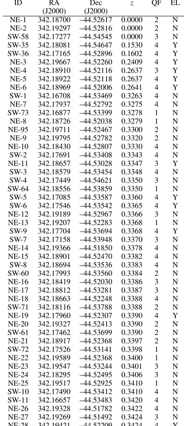
Table 1. LAEs behind AS1063, see TableA.1for quality flags and a cross correlation with multiple images.

ID RA (J2000) Dec (J2000) z NE-91 342.19238 –44.52505 2.9760 SW-49a 342.17505 –44.54102 3.1169c,e SW-49b 342.17315 –44.53999 3.1169a,b,c,e, f SW-50 342.16225 –44.53829 3.1160 SW-68a 342.18745 –44.53869 3.1166a,h SW-68b 342.17886 –44.53587 3.1166a,h NE-93a 342.18283 –44.52028 3.1690 NE-93b 342.19196 –44.52409 3.1690 SW-51 342.17402 –44.54124 3.2275 NE-94a 342.18935 –44.51871 3.2857 NE-94b 342.19615 –44.52291 3.2857 NE-96 342.19709 –44.52483 3.4514 NE-97 342.19100 –44.52679 3.7131 SW-52a 342.18150 –44.53936 4.1130c SW-52b 342.17918 –44.53870 4.1130c NE-98a 342.19015 –44.53093 5.0510 NE-98b 342.19085 –44.53566 5.0510 NE-99a 342.18378 –44.52122 5.2373 NE-99b 342.18874 –44.52276 5.2373 NE-100 342.19701 –44.52212 5.8940 SW-53a 342.18106 –44.53462 6.1074b,c,g SW-53b 342.19088 –44.53747 6.1074b,c,g NE-118c† 342.18402 –44.53159 6.1074 NE-118d† _{342.18904 –44.53004 6.1074} SW-70a 342.18586 –44.53883 3.6065 SW-70b 342.17892 –44.53668 3.6065

Notes. The last galaxy, SW-70, is no LAE, but a Lyman Break galaxy with minimal Lyα emission, and is therefore not considered in the remainder of this paper. Previous redshift determinations by:

(a) _C16;(b) _{Balestra et al.(2013);}(c)_{Paper I;} (d)_{Richard et al.(2014);}

(e) _{Vanzella et al. (2016a);} ( f ) _{Johnson et al. (2014);} (g) _{Boone et al.}

(2013); and (h)_{Caminha et al.(2016a).} (†)_{NE-118 is the same image}

family as SW-53 but located in the NE rather than the SW. To avoid confusion with object NE-53, we listed the objects with the NE-118 identifier.

line emitter which we associate with Lyα emission at z= 5.894, which has no clear counterpart in the FF images. The lensing model predicts additional images outside of the observed MUSE field, but their magnifications are too low to be detected in the HST images. The addition of 2 and possibly 3 spectroscopically confirmed systems at z > 5 should help to further constrain the cosmological parameters, seeC16, while the increased number of z= 3−4 images will decrease the degeneracies and uncertain-ties in the models. We corrected all properuncertain-ties in the main body of this paper for gravitational lensing magnification, using the model described in AppendixB.

Due to lensing distortions, most of the galaxies discussed here have irregular morphologies in the image plane. To opti-mise the S/N of the Lyα line, we created a spatial mask for each source, and extracted the spectrum within this mask. Each mask was constructed by collapsing the cube over the spectral width of the Lyα line, smoothing this stacked image by a 3 pixel wide boxcar function, and masking out every pixel with values <5σ off the background. We verified that this effectively masked out nearby contaminating sources, while also selecting the entire re-gion of Lyα emission.

In Fig.3, we show the observed line profiles of all LAEs discovered in the datacubes, uncorrected for magnification. It is

clear from this figure that the observed fluxes vary widely, from very bright (SW-49) to very faint (NE-97) Lyα lines. We see that all profiles have an asymmetry typical for Lyα lines, and most show a clear smaller blue peak or suggest the presence of a small blue peak. The width of the lines varies amongst our sample, but we find that most LAEs have narrow emission lines. Such narrow lines suggest the presence of low column density gas, and are suggested to be candidate Lyman continuum emitters (e.g. Jones et al. 2013;Verhamme et al. 2015;Vanzella et al. 2016a; Dijkstra et al. 2016).

3.1. Physical properties deduced from Lyα

The LAEs studied here belong to the intrinsically-faintest galaxies ( fλ = 36−2500 × 10−20 erg s−1cm−2) spectroscopi-cally confirmed at these redshifts, see Fig. 5. We measured the Lyα luminosity by summing the flux over the spectro-scopic width of the Lyα line, and subtracting the average of uncontaminated spectral regions redwards and bluewards of Lyα. Subsequently, we used our lensing models to correct the luminosities for the magnifications due to the galaxy cluster, see TableC.1for the adopted magnification factors. The errors on the magnifications are typically of the order of 5–10%, which are generally larger than the photometric errors. For clarity, we have not propagated the errors on our magnification into our error es-timates of other properties in any table or figure. An additional error based on the magnification is therefore applicable for flux derived properties, such as luminosities and stellar masses.

As we have multiple images for some galaxies, we can per-form a test on our luminosities and magnifications. We com-pared the obtained luminosities for these objects, and used the mean luminosity when they agreed within 2σ. For those sources where a larger difference was found, we reinvestigated the dat-acube, and found that the lower-luminosity objects were under-estimated. For two of these, the underestimation was due to the proximity of the edge, which resulted in only a partial coverage. For 3 other objects, contamination by nearby cluster members re-sulted in an oversubtraction of the continuum, while for 1 object a lower S/N in combination with proximity to a skyline resulted in lower fluxes.

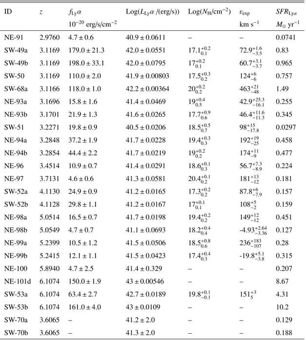
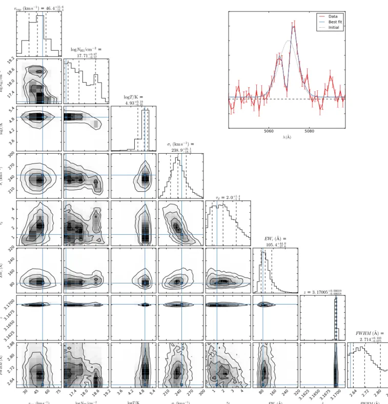
3.1.1. Line profile modelling

In addition to LLyα, we used our spectra to obtain physical

properties of the gas surrounding these faint galaxies. We used the Lyα line fitting pipeline described in detail inGronke et al. (2015) which consists of a pre-computed grid of Lyα radiative transfer models on an expanding shell and a Bayesian fitting framework.

The expanding shell model (first used by Ahn et al. 2003) consists of a central Lyα (and continuum) emitting source sur-rounded by an outflowing shell of hydrogen and dust. Such a model has six free parameters: two describing the photon emit-ting source (the intrinsic line width σi and equivalent width

EWi), three for the shell content (the neutral hydrogen column

density NHi, the dust optical depth τdand the effective

tempera-ture T which includes the approximate effect of turbulence) and the outflow velocity vexp.

The pre-computed grid mentioned above consists of 10 800 models11 _{covering the three parameters T , N}

Hi and vexp

as they shape the spectrum in a complex, non-linear fashion

11 _{The spectra can be accessed online at http://bit.ly/}

0

2

4

6

8

10

NE-91

SW-49

SW-50

SW-68

0

2

4

6

8

10

NE-93

SW-51

NE-94

NE-96

0

2

4

6

8

10

NE-97

SW-52

NE-98

NE-99

1200 1210 1220 1230

0

2

4

6

8

10

NE-100

1200 1210 1220 1230

SW-53

1200 1210 1220 12301200 1210 1220 1230

f

λ

(

10

− 18

er

g

s

− 1

cm

− 2 ◦

A

− 1

)

λ

_Em

(

◦

A

)

Fig. 3.Lyα lines for the LAEs extracted from the MUSE datacube, shown by the blue lines. The spectra are shifted to restframe wavelengths, and

the fluxes are not corrected for the gravitational magnification. The grey bands show wavelengths with significant sky interference, while the black dashed line shows the restframe wavelength of Lyα. The systemic redshifts of LAEs SW-49 and SW-68 have been determined from the narrow UV-emission lines, while we adopted the redshifts based on the Lyα line for the other objects.

5000

6000

7000

8000

9000

Observed wavelength (

◦

A

)

0

20

40

60

80

100

120

Flu

x (

10

− 20

er

g

s

− 1

cm

− 2 ◦

A

− 1

)

1200

1400

1600

1800

Emitted wavelength (

◦

A

)

CIII

_Ly

α

NV SiII

OI

CII

_SiIV

_{SiII CIV}

_FeII

_{HeII OIII] OIII] AlII}

_{NiII NIV NiII NiII}

SiII

SiI AlIII AlIII

CIII

_[NII]

_[NII]

_[NII]

z: 3.6063

Fig. 4.Spectrum of object SW-70a, a newly identified LBG in the SW of AS1063. The spectrum has been smoothed for illustrative purposes, the

0 1 2 3

_z

4 5 6 7 1039 1040 1041 1042 1043 1044

L

Lyα

[e

rg

/s]

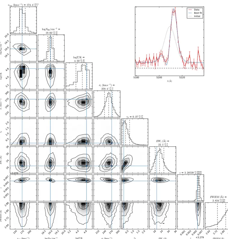
Shimasaku+2006 Dawson+2007 Ouchi+2008 Rauch+2008 Sawicki+2008 Verhamme+2008 Blanc+2011 Cowie+2011 Kashikawa+2011 Curtis-Lake+2012 Henry+2012 Mallery+2012 Wofford+2013 Erb+2014 Hayes+2014 Hashimoto+2015 Henry+2015 Trainor+2015 This work

Fig. 5.Delensed luminosity of the Lyα line against the redshift of our

targets, marked by the red stars. We compare this to previously large samples of spectroscopically-confirmed LAEs in the literature, which are shown by dots of different colours. We overplot the values of L?at various redshifts fromOuchi et al.(2008) with a black dashed line.

(Verhamme et al. 2015). The grid was created using the radia-tive Monte Carlo code tlac (Gronke & Dijkstra 2014) which traces individual photon packages in real- and frequency space (for a comprehensive review on Lyα radiative transfer see, e.g., Dijkstra 2014).

The effect of the remaining three parameters is modelled in post-processing by assigning a weight to each individual photon packet, which means that the procedure affects the shape of the line and not only the normalization. This strategy does not only save computational time but allows to model these parameters continuously, and thus, leads to a more precise sampling of the likelihood when comparing the modelled data to observations.

The actual fitting procedure is done by sampling the Gaus-sian likelihood using the affine invariant Monte-Carlo sampler emcee (Foreman-Mackey et al. 2013) using 400 walkers and 600 steps12_{. In addition to the minimal set of the six shell-model} parameters, we also fit simultaneously for the redshift z and the full-width at half maximum of the Gaussian smoothing ker-nel FWHM. Note that the former adds immense complexity to the fitting procedure as shifting z by a small fraction can alter the quality of the fit tremendously. We used the redshift esti-mate from UV emission lines if available or otherwise the red-shift of Lyα with an intrinsic uncertainty of ∼200 km s−1 _(see

Sect.3.1) as a prior. Alternatively, the latter, i.e. smoothing the spectrum, makes the likelihood function better behaved. How-ever, the width of the smoothing kernel is a function of the ac-tual size of the Lyα halo as well as the measurement aperture. Therefore, we used an allowed range for FWHM corresponding to the wavelength-dependent spectral resolution of the MUSE instrument.

Gronke et al. (2015) discussed the uncertainties of using Lyα line profile fitting for various effects, for example morphol-ogy and signal-to-noise ratio. They showed that the expansion velocity and column density can be recovered reasonably well in most cases, while degeneracies and uncertainties are more prominent among the other parameters. Therefore, we focus in this paper on these two quantities, although we give the full fit-ting results in AppendixD. This is, to our knowledge, the first

12 _{For particularly difficult, multi-modal cases we used a parallel}

tem-pered ensemble MCMC sampler (for a review see,Earl & Deem 2005) with 20 temperatures, 50 walkers and 3000 steps.

1040 ₁₀41 ₁₀42 ₁₀43 ₁₀44

L

Lyα

[erg s

−1

]

17 18 19 20 21

Lo

g(

N

H

/cm

− 2

)

Verhamme+2008 Hashimoto+2015 This work

Fig. 6.Delensed luminosity in Lyα against the column density

deter-mined from modelling the Lyα profile. Legend and symbols are as in Fig.5.

time that the gaseous properties of such faint sources are studied through Lyα modelling. Therefore, this presents one of the first studies to determine the effect star formation has on gas in these faint galaxies.

3.1.2. Shell properties

We modelled the Lyα profiles of 12 LAEs using the approach de-scribed above yielding excellent fits to the observed Lyα spectra (see Appendix D). We present the properties based on the Lyα line in Table2, where we already combined the multiple images into a single result. We modelled the Lyα line profile of each image, and combined the results of each modelling into a single result per LAE. We used the average of all images, af-ter discarding multiple images which were possibly affected by close galaxies or artefacts in the datacube. We did not include 2 LAEs in the modelling, as their Lyα lines were too faint and spectrally unresolved.

In Fig. 6, we show that the column density of the expand-ing shell is low in all of the galaxies. InVanzella et al.(2016a) we reported the results of Lyα line modelling for SW-49 us-ing higher resolution X-shooter spectra and an updated shell-model fitting pipeline. We find that the MUSE and X-shooter results are broadly consistent within the error bars, although we used a larger database reaching lower column densities for the X-shooter spectrum.

We compare the best fit column densities in our sample to those found byVerhamme et al.(2008) andHashimoto et al. (2015), who also fit Lyα profiles with expanding shell mod-els. With all except one LAE best fit with Log(NH/cm2) < 20

and only five LAEs with Log(NH/cm2) > 19, we find lower

column densities than the other studies. However, the galaxies studied here are also ∼1 dex fainter than the ones presented in Verhamme et al.(2008) andHashimoto et al.(2015).

These low column densities support the idea that for these faint galaxies, the Lyα is not significantly broadened by scatter-ing. This is consistent with the picture that Lyα escape becomes easier for fainter galaxies with significant Lyα emission.

We find no trends in the velocity of the expanding shell with the Lyα luminosity, but we note that we find relatively low outflow velocities in all galaxies. The absence of a correlation

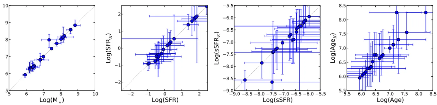
Table 2. Properties derived from Lyα spectroscopy, after averaging results for multiple images.

ID z fLyαa Log(LLyα/(erg/s))b Log(NH/cm−2)c vexpd

10−20_erg/s/cm−2 NE-91 2.9760 108 ± 14 40.91 ± 0.06 – – SW-49 3.1166 1080 ± 129 41.91 ± 0.06 17.07+0.26_−0.03 66.78+7.07_−6.11 SW-50 3.1169 984 ± 18 41.92 ± 0.01 17.53+0.24_−0.23 123.63+6.57_−5.85 SW-68 3.1166 1942 ± 16 42.22 ± 0.01 20.01+0.20_−0.25 463.18+20.40_−48.58 NE-93 3.1690 431 ± 26 41.58 ± 0.02 18.36+1.16_−0.65 44.65+27.91_−1.79 SW-51 3.2271 36 ± 2 41.24 ± 0.01 18.53+0.50_−0.71 97.99+14.63_−17.76 NE-94 3.2857 524 ± 27 41.70 ± 0.02 19.22+0.37_−0.20 183.33+23.37_−8.92 NE-96 3.4514 228 ± 15 41.39 ± 0.03 18.59+0.14_−0.25 56.68+7.35_−8.85 NE-97 3.7131 155 ± 19 41.30 ± 0.06 20.39+0.09_−0.14 180.58+13.00_−12.00 SW-52 4.1130 106 ± 4 41.24 ± 0.02 17.12+0.32_−0.17 98.10+12.93_−10.29 NE-98 5.0510 186 ± 8 41.70 ± 0.02 19.42+0.22_−0.21 149.27+11.83_−11.83 NE-99 5.2373 113 ± 11 41.47 ± 0.05 17.99+0.97_−0.56 107.87+223.75_−127.68 NE-100 5.8940 60 ± 32 41.36 ± 0.33 – – SW-53 6.1074 2694 ± 67 43.04 ± 0.01 19.81+0.07_−0.08 150.56+3.69_−4.1

Notes. The columns are(a)_{lens-corrected Lyα flux;}(b)_luminosity;(c)_{the hydrogen column density, and}(d)_{expansion velocity.}

Table 3. Parameter space used for constructing stellar templates used in our SED fitting.

Range Nr. steps

Age 0.01 Myr–2.3 Gyr 50

E(B − V) 0–1.5 20

Z 0.0004–0.02 (Z) 4

τ 0.001 Gyr–5 Gyr 5

Notes. The stepsizes are logarithmic distributed for the ages, while we use an irregular spacing for the stepsizes of E(B − V) where we finely sample the low values, and use larger steps for the higher values. The metallicities correspond to the m32, m42, m52 and m62 models of BC03.

between the Lyα luminosity and the expansion velocity of the shell is unexpected, as both are considered to correlate with the SFR (e.g. Weiner et al. 2009; Bradshaw et al. 2013; Chisholm et al. 2015). A possible explanation could be that the outflow speed does not follow the SFR at low masses, see below, or that the Lyα luminosity depends more strongly on the escape fraction of Lyα photons than on the SFR.

4. Stellar properties

We used the constructed photometric catalogue in combination with the spectroscopic redshifts to perform a spectral energy dis-tribution (SED) fitting on our selected sample. We used LeP-hare (Arnouts et al. 1999;Ilbert et al. 2006) in combination with Bruzual & Charlot (2003, hereafter BC03) templates to fit the photometry with stellar population models (see Table3for our model parameters). The set of stellar populations consists of an exponentially declining star formation histories, SFR(t) = SFR0 × e−t/τ, with different values for τ. In addition, we

cre-ated templates with three different metallicities, and ages up to

the age of the Universe. We used aCalzetti et al.(2000) extinc-tion curve to attenuate all stellar templates, with 0 < E(B − V) < 1.5. We enabled adding nebular emission lines to the templates based on their UV luminosity as described inIlbert et al.(2009), where the line fluxes of [O

_ii

] λ3727 are derived using the current SFR, and [O

_iii

] λλ4959, 5007, H α, and H β are then scaled from locally derived line ratios. The addition of emission lines to stellar-population templates is shown to be important in the high-redshift Universe (e.g.Schaerer & de Barros 2009; de Barros et al. 2014).

We fitted the SED of each image and combined the re-sults of the multiple images in a similar method as for the Lyα luminosities and Lyα line fitting. We used the average re-sults of multiple images when the quality of the photometric data of each image is similar, but adopt the results of only the best constrained image if the difference is significant, for exam-ple for NE-94 we only used image a. For galaxies where we sus-pect contamination from nearby galaxies, for example SW-68b, we used only the images without contamination. We performed tests on the reliability of our results in AppendixC, and found that although there are few constraints in the restframe optical, our results do not change significantly.

We present the results from the SED fitting in Table4. We remind the reader that most of the photometry is in the frame UV, but that the Hawk-I and IRAC filters trace the rest-frame optical. We detected 6 LAEs in the K-band and 1 LAE in the IRAC filters, but the non-detections provide important upperlimits when determining stellar masses and show that there is no hidden dominant old population of stars.

The masses we derived from our SED fitting are very low, varying from ∼106_M

to ∼108 M, significantly lower than the

stellar masses explored in previous studies of LAEs. This is not surprising, as these galaxies are among the intrinsically faintest discovered so far with absolute UV-magnitudes ranging form – 19 to –14, and illustrates once more the advantages of gravita-tional lensing. We note that for 2 LAEs discovered here (NE-99

Table 4. Stellar properties derived from SED modelling using L

_e

P

_hare

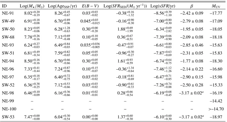
in combination with BC03 templates.

ID Log(M?/M) Log(AgeSSP/yr) E(B − V) Log(SFRSED/(Myr−1)) Log(sSFR/yr) β MUV

NE-91 8.02+0.20_−0.19 8.26+0.45_−0.67 0.03_−0.02+0.03 –0.38+0.16_−1.32 –8.56+0.39_−1.10 –2.42 ± 0.09 –17.77 SW-49 6.91+0.18_−0.08 6.70+0.89_−0.06 0.045_−0.015+0.03 –0.16+0.90_−0.30 –7.00+0.80_−0.30 –2.79 ± 0.08 –17.09 SW-50 8.23+0.05_−0.06 6.28+1.28_−0.63 0.30_−0.20+0.00 1.88+0.69_−1.99 –6.34+0.69_−2.82 –1.95 ± 0.05 –18.05 SW-68 7.78+0.26_−0.16 7.12+0.69_−0.48 0.10_−0.05+0.10 0.36+0.67_−0.51 –7.39+0.66_−0.90 –2.09 ± 0.08 –18.18 NE-93 6.24+0.27_−0.03 6.49+0.84_−0.03 0.035_−0.005+0.036 -0.47+0.91_−0.07 –6.61+0.80_−0.03 –2.85 ± 0.46 –15.63 SW-51 6.81+0.49_−0.34 7.59+0.82_−0.65 0.05_−0.03+0.05 –0.96+0.30_−0.27 –7.87+0.63_−0.69 –2.31 ± 0.05 –15.83 NE-94 8.50+0.16_−0.16 6.70+0.66_−0.66 0.30_−0.05+0.05 1.61+0.93_−0.59 –6.74+0.64_−0.75 –1.77 ± 0.08 –18.30 NE-96 7.33+0.41_−0.44 7.24+0.87_−0.96 0.10_−0.07+0.15 –0.36+1.34_−0.64 –7.46+1.12_−1.26 –2.14 ± 0.22 –16.60 NE-97 6.35+0.18_−0.17 6.40+0.72_−0.75 0.03_−0.02+0.03 –0.18+0.81_−0.69 –6.47+0.71_−0.85 –2.90 ± 0.15 –15.98 SW-52 6.36+0.38_−0.25 7.12+0.53_−0.66 0.03_−0.02+0.03 –0.90+0.61_−0.33 –7.26+0.74_−0.88 –2.50 ± 0.28 −15.33 NE-98 6.46+0.10_−0.09 6.16+0.36_−0.66 0.01_−0.01+0.02 0.28+0.66_−0.54 –6.19+0.68_−0.45 –3.17 ± 0.02a _–16.19 NE-99 – – – – – – –14.42 NE-100 – – – – – – >–14.70 SW-53 7.47+0.00_−0.00 6.04+0.30_−0.54 0.00_−0.00+0.00 1.37+0.60_−0.30 –6.10+0.60_−0.30 −3.17 ± 0.02a _–18.97

Notes. The properties were derived after averaging the results of multiple images of the same source, if applicable. See AppendixCfor results of all individual LAEs.(a)_{This is the maximal UV slope in our used templates, the photometric UV-slope is steeper and the small errors are therefore}

not representative but a result of our method of calculating β.

and NE-100), we recovered only a single detection through all deep FF filters, which is in the filter containing Lyα. The com-pletion of the NIR-imaging of AS1063 in the summer of 2016 should add more detections to these objects, and will better con-strain the properties of these possibly even less massive galaxies. In Fig.7, we compare the stellar masses of our galaxies to their Lyα luminosities. We see that the lower masses are paired with lower luminosities. The low luminosities and masses found here in comparison to previous literature results confirm again that these objects probe a new region of parameter space.

The presence of such narrow and strong Lyα emission is al-ready a clear indication that there is little dust present. We find that the median marginalised E(B − V) values are all very small, with only 3 galaxies having E(B − V) > 0.1, in agreement with previous studies (e.g.Atek et al. 2014).

The ages of these very low mass objects are relatively low, that is 1–100 Myr, see Fig.8. We find that only two galaxies have an age >100 Myr, and age seems to decrease with redshift. The young stellar ages indicate that these are systems that are rapidly building up their mass. This is confirmed by the SFR that we ob-tain given the low stellar masses, see Fig.9, as with the current SFR, most galaxies will double their mass within 107 _{yrs. As a}

consequence of these young ages, the models produced by dif-ferent values of τ are very similar. Therefore, the current data are unable to distinguish between the different star formation histories.

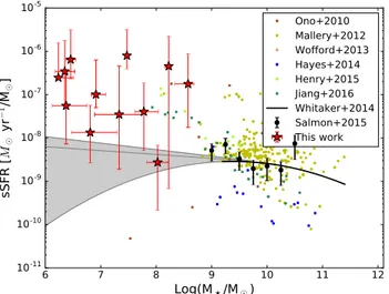
We compare the SED-derived SFR to the SFR extrapolated from the SFR-stellar mass relation determined for more mas-sive galaxies, both at lower and similar redshift. We find that most of the LAEs fall above this relation if an extrapolation of the power-law relation described by Whitaker et al. (2014) is considered. Because very little is known about the SFR in

6 7 8 9 10 11

Log(M /M

¯

)

1040 1041 1042 1043 1044

L

Lyα

[e

rg

/s]

Fig. 7.Stellar mass versus the lens-corrected Lyα luminosity. The LAEs

described here are compared to a collection of previous LAE studies, with the colours identical to Fig.5, where we have supplemented the results fromBlanc et al.(2011) with those ofHagen et al.(2014).

low mass galaxies, this extrapolation is rather uncertain due to a degeneracy between the slope of the power-law and its zero-point. If we use the steep power-law relation described for z ∼ 4 galaxies by Salmon et al. (2015), the number of LAEs above this relation will decrease by a factor 2. We note however, that many studies favour a slope of α= 1 (e.g.González et al. 2010; Whitaker et al. 2014;Ilbert et al. 2015), which would make most of these LAE starbursting galaxies.

6 7 8 9 10 11 12

Log(M /M

¯

)

5 6 7 8 9 10

Lo

g(

Ag

e

SSP

/y

r

)

Ono+2010 Hagen+2014 Mallery+2012 Wofford+2013 Hayes+2014 McLinden+2014 Finkelstein+2015 Jiang+2016 Composites This work

Fig. 8.Stellar mass versus the age of the stellar population, as

deter-mined by SED-fitting of exponentionally declining star formation histo-ries. The coloured dots correspond to a variety of results from previous spectroscopically-confirmed LAE studies, while the grey squares cor-respond to the collection of composites assembled byMcLinden et al.

(2014). For comparison, we also plot a sample of non-LAE, represented by the pink dots (Finkelstein et al. 2015).

6 7 8 9 10 11

Log(M /M

¯

)

10-2 10-1 100 101 102 103

SF

R

[

M

¯

yr

− 1

]

Ono+2010 Mallery+2012 Wofford+2013 Hayes+2014 Henry+2015 Salmon+2015 z=4 Whitaker+2014 This work

Fig. 9.Stellar mass versus the star formation rate. See Fig.10for a

de-scription of the different studies. The black dots and dark grey region correspond to the SFR for galaxies in CANDELS at z ∼ 4 as deter-mined bySalmon et al.(2015), while the black dashed line presents an extrapolation to lower masses based on these data. We show the SFR for a sample of z = 2.0−2.5 galaxies fromWhitaker et al.(2014) and three possible extrapolations to lower masses with the black line and three grey lines respectively.

To have a clearer understanding of whether these faint LAEs are normally star forming or starbursting, we looked at the spe-cific SFR (sSFR= SFR/M?). We find that in our sample of LAEs the average sSFR is significantly higher than seen in other LAE samples, see Figs.10and11. This shows that these galaxies are not only young, but are still actively forming stars. The sSFR classifies these galaxies as starburst galaxies, if one assumes the flat sSFR-M? correlation found for stellar masses M? < 109

(González et al. 2010; Whitaker et al. 2014; Ilbert et al. 2015). However, whether this relation is flat at these redshifts is un-known, as this mass range has not been explored before even at low redshift.

Similarly high sSFRs are rarely found in any other sources. For more massive sources at high-redshift with young ages,

0 1 2 3 4 5 6 7

z

10-12 10-11 10-10 10-9 10-8 10-7 10-6 10-5

sS

FR

[M

¯

yr

− 1

/M

¯

]

Ono+2010 Mallery+2012 Wofford+2013 Hayes+2014 Henry+2015 Jiang+2016 This work

Fig. 10.Specific SFR as a function of redshift. The sSFR of our

sam-ple,Ono et al.(2010),Mallery et al.(2012), andWofford et al.(2013) is

calculated using only SED fitting, forHayes et al.(2014),Henry et al.

(2015) the sSFR is calculated using the SFR based on Hα, and the sSFR

ofJiang et al.(2016) is calculated using SFRUV. The black line shows

the sSFR of the CANDELS galaxies fromSalmon et al.(2015).

6 7 8 9 10 11 12

Log(M /M

¯

)

10-11 10-10 10-9 10-8 10-7 10-6 10-5

sS

FR

[

M

¯

yr

− 1

/M

¯

]

Ono+2010 Mallery+2012 Wofford+2013 Hayes+2014 Henry+2015 Jiang+2016 Whitaker+2014 Salmon+2015 This work

Fig. 11.Stellar mass versus the specific star formation rate. See Figs.10

and9for a description of the different studies and legend.

a typical log (sSFR)= –8 is found (e.g González et al. 2010; Stark et al. 2013;Oesch et al. 2015,2016;Tasca et al. 2015), al-thoughOno et al.(2012) and Finkelstein et al. (2013) report a similarly high sSFR at z > 7. Extreme emission line galax-ies (EELGs) at lower redshift show similar values on average, but the spread is large enough that the upper envelope contains some galaxies with log(sSFR) > −7.5 (Cardamone et al. 2009; Amorín et al. 2014,2015;Maseda et al. 2014;Ly et al. 2014). A comparable evolution of the sSFR with redshift as seen in nor-mal galaxies (seeSpeagle et al. 2014, for a recent compilation), could bring the EELGs up to a similar sSFR found in our sam-ple, strengthening the possible link between EELGs and high-redshift LAEs.

We compared the sSFR to all other parameters, but find no further correlations with neither any gaseous nor any stellar property. Even the apparent trend of an increasing sSFR with in-creasing LLyαwithin our sample disappears when other studies

are added, see Fig.12. This suggests that the sSFR has no influ-ence on the Lyα line profile or the physics that shape the line,

10

40

₁₀

41

₁₀

42

₁₀

43

₁₀

44

L

Lyα

[erg/s]

10

-11

10

-10

10

-9

10

-8

10

-7

10

-6

10

-5

sS

FR

[M

¯

yr

− 1

/M

¯

]

Fig. 12. Lyα luminosity versus the specific star formation rate. See

Fig.10for a description of the different studies.

nor is the sSFR influenced by any other stellar parameter than the stellar mass and age. It is noteworthy that in several of these plots we find higher sSFR within our sample when compared to other samples at a given property. This further suggests that the high sSFR is driven by the low stellar mass and young age.

Most galaxies, except two (SW-50 and SW-51), are best fit with a low metallicity, however a solar metallicity falls within our 1σ certainty range for most of the LAEs. A low metallicity for most of these galaxies would be in agreement with all pre-vious results that these are recently formed, low-mass galaxies which are rapidly building up mass and have not been able to produce a large amount of metals.

4.1. Lyα escape fraction

To understand the evolution and formation of the Lyα luminosity function and the process of reionization it is important to determine how much of the Lyα flux escapes the galaxy. To estimate this, we follow previous studies, using the UV or SED derived SFRUV/SED and compare these to the

SFR calculated from Lyα (SFRLyα) to define the escape

fraction fesc= SFRLyα/SFRSED. We determine SFRLyαfollowing

Kennicutt(1998) and assuming case B recombination:

S FRLyα(Myr−1)= LLyα(erg s−1)/8.7 × 7.9 × 10−42. (1)

We caution the reader that this relation has been calibrated on stable star forming galaxies and that this may not be applicable at very young ages.

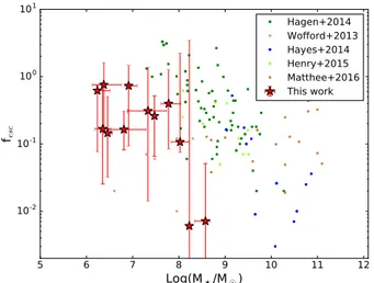
In Fig.13 we show the Lyα escape fraction as a function of stellar mass. We find higher escape fraction for lower stellar masses, a trend which remains visible after other studies are in-cluded. We note, however, that this trend is also a natural effect of the selection bias when studying LAEs. Galaxies with low es-cape fractions will have very little or no Lyα emission, and will therefore remain undetected in emission line studies, whereas low mass galaxies will evade detection in the continuum. These effects would produce a trend similar to the one observed here, however, the dearth of massive galaxies with high-escape frac-tions is genuine and cannot be explained by selection effects. 4.2. UV-continuum slope

We used the best-fitting SED model to measure β, the slope of the UV spectrum defined as fλ ∝ λβ (e.g.Meurer et al. 1999),

5 6 7 8 9 10 11 12

Log(M /M

¯

)

10-2 10-1 100 101

f

esc Hagen+2014 Wofford+2013 Hayes+2014 Henry+2015 Matthee+2016 This work

Fig. 13. Lyα escape fraction versus the stellar mass. We followed most

studies and used the indirect fesc= SFRLyα/SFRSED, whileHayes et al.

(2014) andHenry et al.(2015) used the flux ratio of Lyα to Hα to di-rectly derive fesc.

following Finkelstein et al. (2012). We chose to use the best-fitting SED model to measure β rather than observed colours as this was shown to be a more stable approach (e.g. Finkelstein et al. 2012; Bouwens et al. 2014). We adopted the spectral windows defined byCalzetti et al.(1994), and directly fitted a power law to the best-fitting template in these windows. We find a clear relation between the stellar mass and β, see Fig.14, in agreement with previous results (e.g.Bouwens et al. 2014). For each galaxy, we derive the uncertainty of β by repeat-ing the full-SED modellrepeat-ing for 1000 mock galaxies, created by randomly disturbing its photometry taken from a normal random distribution based on the photometric errors. Because the mini-mum value of β ≈ −3.2 for BC03 models with a Chabrier IMF, galaxies with photometric slopes bluer than this will almost al-ways be best fitted with β= −3.2, even after scattering the pho-tometry. This leads to unrealistically small errors for some of our UV-slopes, for example NE-98. We then fitted a Gaussian to the distribution of β of all mock galaxies, and report the resulting σ as the uncertainty in β. We calculated the slope of the β-mass relation to be 0.43 in our sample, comparable to the maximum slope of 0.46 at z= 7 byFinkelstein et al.(2012). We note how-ever, that the majority of our samples lies at 3 < z < 4, for which Finkelstein et al.(2012) found a slope of only 0.17. An impor-tant factor in this difference could be our selection bias, meaning that we only find galaxies with strong Lyα emission.

Dunlop et al.(2012) argued that very blue UV slopes could be caused by low S/N photometry. In this study however, we do not suffer from uncertainties in redshift, which are the largest factor in the scatter of β in photometric studies. Therefore, we do not expect to be affected by the same bias. The very blue slopes are also in agreement with the low stellar masses, low dust extinction, and young ages found in these LAEs, as also discussed for example byDunlop et al.(2012).

Jiang et al. (2016) measured the UV-slope of their sample of LAEs, and they find a significant number of more massive LAEs with very blue slopes. This seems to be in disagreement with our and other previous results, as they would predict that more massive galaxies have redder continua due to a higher metallicity and larger amounts of dust. This is possibly due to low S/N photometric data available for the relevant sources in Jiang et al.(2016), leading to a larger scatter found in the β slope (Dunlop et al. 2012). Another possible explanation for this is

5.5 6.0 6.5 7.0 7.5 8.0 8.5 9.0 9.5 10.0

Log(M /M

¯

)

3.5 3.0 2.5 2.0 1.5 1.0 0.5

β

van der Wel+2011 Hagen+2014 Henry+2015 Jiang+2016 Finkelstein+2012 This work

Fig. 14. Stellar mass versus the UV-continuum slope β. We

over-plotted a number of LAEs from Hagen et al. (2014), Henry et al.

(2015), andJiang et al.(2016), the median of CANDELS galaxies at z = 4 fromFinkelstein et al. (2012), and a sample of EELGs from

van der Wel et al.(2011).

that the number density of blue more-massive LAEs is signifi-cantly lower than those of slightly redder LAEs. Because we are only observing a rather small volume, this means that the very low number of blue massive LAEs in our sample is expected.

We note that for a few of our LAEs, we find the steepest theoretically-allowed β for pure stellar populations without a nebular contribution, that is β = −3.17. In these cases, the ob-servations are representative of an even steeper slope, and, nat-urally, models with flatter continuum slopes are disfavoured by SED fitting. A steeper UV continuum than the theoretical max-imum value for stellar templates β < −3.2 can be achieved by including the effects of a nebular continuum into the SED fitting (e.g.Schaerer & de Barros 2009;Zackrisson et al. 2013) or by using top-heavy IMFs or Pop III stars (e.g.Bouwens et al. 2010; Zackrisson et al. 2011).

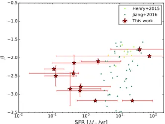
A steep UV-continuum slope is associated with young and rapidly star forming galaxies without a significant amount of dust. Therefore, one would expect that β might correlate with the SFR. We show the comparison between SFR and β in Fig.15, but we see that there is no obvious correlation between the two either in our sample, or in either of the other samples. The lack of a clear relation between SFR and β in our sample could pos-sibly be due to the large uncertainty in the SFR derived from SED modelling, however, it has also been found in other studies. A physical reason for the absence of a correlation could be that the metallicity, and therefore the dust opacity, is not as strongly correlated with SFR as with stellar mass.

4.3. Linking gas to stars

We now compare the stellar properties derived from the broad-band photometry to the gaseous properties derived from the Lyα line profile modelling. First, we compare the expansion velocity to the sSFR in Fig. 16. We find no clear relation be-tween these two quantities, see Sect.5for a discussion on this.

A more interesting result is found when we compare the col-umn density to the stellar mass, see Fig.17. On the one hand, we see that the column density found byHashimoto et al.(2015) us-ing shell model fittus-ing to z ∼ 2.2 LAEs is similar to those found here, but at significantly higher stellar mass. On the other hand, the stellar masses of the z ∼ 0.03 LAEs inWofford et al.(2013), who use UV absorption line modelling for LBGs, are similar to

10-2 ₁₀-1 ₁₀0 ₁₀1 ₁₀2

SFR [

M¯

/yr]

3.5 3.0 2.5 2.0 1.5 1.0 0.5

β

Henry+2015 Jiang+2016 This work

Fig. 15.SFR versus the UV-continuum slope β. We overplotted a

num-ber of LAEs fromHenry et al.(2015) andJiang et al.(2016).

100 0 100 200 300 400 500

v

exp

[km/s]

10-12 10-11 10-10 10-9 10-8 10-7 10-6 10-5

sS

FR

[

M¯

yr

− 1

/M

¯

]

This work

Fig. 16.Expansion velocity, derived from Lyα line modelling, against

the sSFR, derived from SED fitting.

the ones discussed here, but the column densities are two orders of magnitude larger. The difference could be a consequence of the different redshifts, as low column density objects are at rel-atively high-redshift when cosmic star formation was peaking, while the high column density refers to galaxies at z < 0.06. This suggests an evolution of the column density of galaxies, although there are several caveats to be considered, see Sect.5. We note, however, that none of the galaxies with column density measures fromWofford et al.(2013) are LAEs, opposed to the sample of Hashimoto et al.(2015) and the one discussed here. The di ffer-ence in column densities at the same mass could therefore simply mean that selecting by Lyα luminosity sets a maximum value on the column density, which is in agreement with the finding of Hashimoto et al.(2015) that the expansion velocity and column density in LAEs are significantly lower than those in LBGs. It was shown bySchaerer et al.(2011) that a high expansion ve-locity vexp > 300 km s−1 is required in galaxies with a high

column density in order to allow the escape of Lyα photons. These high velocities are significantly higher than expected for M?< 108Mgalaxies.

5. Discussion

The absence of a relation between the outflow velocity and the SFR, stellar mass, and sSFR is apparently in contradiction with previous studies (e.g.Weiner et al. 2009;Bradshaw et al. 2013; Erb et al. 2014). The difference in stellar masses could be the

6 7 8 9 10 11 12

Log(M /M

¯

)

17 18 19 20 21 22

Lo

g(

N

H

/cm

− 2

)

Wofford+2013 Hashimoto+2015 This work

Fig. 17.Comparison of the stellar mass to the column density based

on Lyα line modelling. We also plot results from a sample of LAEs analysed in a similar manner by modelling Lyα lines using shell mod-els (Hashimoto et al. 2015), and a sample of LBGs, where the column density is derived from UV absorption line modelling (Wofford et al.

2013).

prime factor between these results, as a burst of star formation can have a much more destructive effect on a low mass galaxy than on a massive galaxy. The low outflow velocities and young ages are in agreement with a scenario where a short violent episode of star formation blows away a shell of gas at moder-ate velocity. In more massive galaxies, the star formation is less episodic, and the velocity needed to expell gas from the galaxy is higher. Therefore, one would expect to see a large scatter with on average very moderate velocities in low mass galaxies, and an increasing trend of outflow velocity with stellar mass at higher masses. We note that all but one velocity reported here are below the velocity of the lowest-mass bin inBradshaw et al.(2013).

We used the expanding shell-model to fit the observed spectra with astonishing accuracy given the complexity of the spectral shape and the relatively few free parameters of the model. This finding is well aligned with previous studies (e.g. Verhamme et al. 2008; Schaerer et al. 2011; Hashimoto et al. 2015;Yang et al. 2016) who found the shell-model to represent also a good fit to the data.

In spite of this success, the shell-model is clearly a simplifi-cation of the complex velocity and density fields existing in high-redshift galaxies and the physical meaning of the shell-model parameters is still unclear. Recently,Gronke & Dijkstra(2016) found that the shell-model parameters do not match the ones of a more complex, multi-phase medium. This hints towards a more subtle conversion between the shell-model and the actual physi-cal parameters. For example,Gronke & Dijkstra(2016) showed that low column densities in shell models can reflect a medium consisting of optically thick clumps of gas with a low covering factor.

Independent of the question whether the parameters can be interpreted literally or are a more abstract quantity, we found several interesting correlations between them and other ob-served quantities. In particular, we found that the spectra can be reproduced best using lower neutral hydrogen column densi-ties in shell models than in previous studies (Verhamme et al. 2008; Hashimoto et al. 2015) which studied brighter galaxies than our sample. This fact combined with the relative large Lyα escape fraction for most of our objects (the Lyα and LyC

escape fractions are expected to correlate, see e.g.,Yajima et al. 2014;Dijkstra et al. 2016), and the low mass (simulations sug-gest larger LyC escape fractions for lower mass galaxies, e.g., Paardekooper et al. 2015) makes our sample ideal candidates for LyC leaking galaxies.

When comparing properties as outflow velocity or column density to other studies, one has to be aware of differences in methods. Modelling Lyα profiles is very sensitive to neutral hy-drogen, but as a large number of different properties of neutral hydrogen are involved, degeneracies arise naturally. For exam-ple, there are strong degeneracies between optical depth and EW, between σi and the temperature of the gas. Perhaps the

most important degeneracy arises between z and a combina-tion of vexpand NH_i, that is a difference in the systematic

red-shift can be compensated by changing the outflowing velocity and the column density or morphology or vice versa. The very consistent results of the Lyα modelling and the outflow veloc-ity and column densveloc-ity determinations from other emission lines (see, Vanzella et al. 2016a) is encouraging. Results from rela-tively comparable samples of galaxies with different techniques strengthen the finding of low outflow velocities for faint LAEs (Erb et al. 2014; Trainor et al. 2015). Running a large number of parametrizations of the properties in combination with con-straining the free parameters by other means helps to minimise the number of degeneracies. Gronke et al. (2015) showed that the column density, expansion velocity, and σ are well recov-ered by these models, indicating that for the properties dis-cussed here the influence of degeneracies is rather low. Other methods of determining the column density in outflows, for ex-ample through absorption line fitting (e.g.Wofford et al. 2013; Karman et al. 2014), are based on several assumptions such as temperature, metallicity, and electron density, which can lead to systematic differences. Although there is currently no evidence for these systematics, these concerns should be taken into con-sideration when comparing different techniques. We therefore caution the reader when we compared our column densities to those ofWofford et al.(2013).

The simplified modelling thus introduces additional uncer-tainties. As mentioned previously, if we are observing the galaxy through one of the holes of a patchy distribution, the mod-elled column density will be underestimated (Gronke & Dijkstra 2016). Further, as star formation occurs stochastic in these low mass galaxies (e.g. Cloet-Osselaer et al. 2014; Hopkins et al. 2014; Maseda et al. 2014; Shen et al. 2014; Domínguez et al. 2015; Guo et al. 2016), it is expected that rather than a single shell, multiple shells are present from the multiple episodes of star formation. It is unclear how much this affects the galaxies studied here, as their ages indicate very young galaxies, prevent-ing a large number of episodes of star formation.

The stochastic nature of low-mass galaxies poses another caveat, as we have here modelled the galaxies with a single expo-nentially decaying star formation history. The very young ages could be a result of a strong recent episode of star formation on top of a more evolved and older stellar population. How-ever, for most of the galaxies, the non-detections in the Hawk-I observations limit a possible contribution of old stellar popula-tions. At the moment, the available data are unfortunately insuf-ficiently deep to directly observe the older population. This is because older populations dominate at longer wavelengths, for which data with similar depth and resolution are currently not achievable.

Although we are including the strongest emission lines in our SED-fitting, we are not including a nebular continuum. The best-fitting models match the observations relatively well in the