Perfezionamento in Matematica
Indirizzo in Scienze Finanziarie e Assicurative
Volatility estimate
via
Fourier analysis
Preface 7
1 Theory of quadratic variation 11
1.1 Quadratic variation . . . 11
1.1.1 Preliminaries . . . 11
1.1.2 Stopping times and subdivisions . . . 12
1.1.3 Martingales . . . 13
1.1.4 Quadratic variation for locally square-integrable martingales . . . 15
1.1.5 Semimartingales . . . 16
1.1.6 Stochastic integral . . . 17
1.1.7 Quadratic Variation . . . 19
1.1.8 Stochastic differential equations . . . 24
1.2 Convergence to a martingale . . . 26
1.3 Estimating quadratic variation . . . 28
1.4 Quadratic variation in financial economics . . . 29
2 Volatility estimate via Fourier Analysis 33 2.1 Univariate case . . . 33
2.2 Multivariate case . . . 40 3
3 Univariate applications 41
3.1 Introduction . . . 41
3.2 Monte Carlo experiments . . . 43
3.2.1 GARCH(1,1) process . . . 44
3.2.2 SR-SARV(1) process . . . 49
3.2.3 Volatility forecasting evaluation . . . 50
3.3 Foreign exchange rate analysis . . . 51
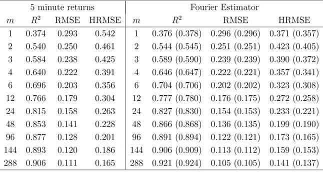
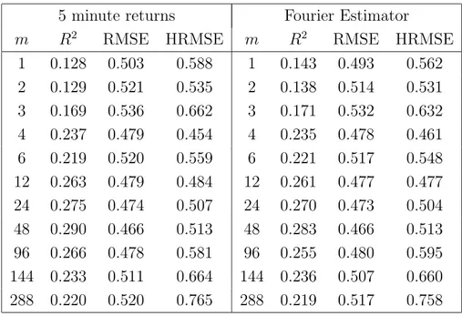
3.3.1 Forecasting daily exchange rate volatility using intraday returns . . . 56
3.4 A linear model for volatility . . . 60
3.5 The volatility of the Italian overnight market . . . 63
3.5.1 The data set . . . 67
3.5.2 Testing the martingale hypothesis . . . 68
3.5.3 Interest rate volatility and market activity . . . 72
3.6 Conclusions . . . 78
4 Multivariate applications 81 4.1 Introduction . . . 81
4.2 Performance on simulated data . . . 82
4.3 Investigating the Epps effect . . . 85
4.3.1 Monte Carlo experiments . . . 86
4.3.2 Data analysis . . . 90
4.4 Dynamic principal component analysis . . . 95
4.4.1 Empirical Results . . . 97
5 Nonparametric estimation 105
5.1 Introduction . . . 105
5.2 Nonparametric estimation of the diffusion coefficient . . . 109
5.3 Small sample properties . . . 116
5.4 Data Analysis . . . 119
5.5 Conclusions . . . 120
T
he aim of this Thesis is to study some selected topics on volatility estimation and modeling. Recently, these topics received great attention in the financial literature, since volatility modeling is crucial in practically all financial applications, including derivatives pricing, portfolio selection and risk management. Specifically, we focus on the concept of realized volatility, which became important in the last decade mainly thanks to the increased availability of high-frequency data on practically every financial asset traded in the main marketplaces. The concept of realized volatility traces back to an early idea of Merton (1980), and basically consists in the estimation of the daily variance via the sum of squared intraday returns, see Andersen et al. (2003). The work presented here is linked to this strand of literature but an alternative estimator is adopted. This is based on Fourier analysis of the time series, hence the term Fourier estimator, which has been recently proposed by Malliavin and Mancino (2002). Moreover, we start from this result to introduce a nonparametric estimator of the diffusion coefficient.The Thesis has two main objectives. After introducing the concept of quadratic variation and the Fourier estimator, we compare the properties of this estimator with realized volatility in a univariate and multivariate setting. This leads us to some applications in which we exploit the fact that we can regard volatility as an observable instead of a latent variable. We pursue this objective in Chapters 3 and 4. The second objective is to prove two Theorems on the estimation of the diffusion coefficient of a stochastic diffusion in a univariate setting, and this is pursued in Chapter 5.
The detailed structure of the work is the following.
In Chapter 1 we review basic facts about quadratic variation, thus we need to introduce semimartingales, stochastic integrals and stochastic differential equations. Moreover, some results on convergence of processes to semimartingales are sketched. The Chapter ends with a brief review of the literature concerning the issues that will be discussed in the subsequent chapters.
In Chapter 2 the Fourier estimator (Malliavin and Mancino, 2002) is introduced and proved to be consistent, both for the univariate and multivariate case. Details on the asymptotic distribution are given in the case of constant variance.
In Chapter 3 we deal with univariate applications. We first compare the Fourier estimator to alternative estimators, mainly realized volatility, on simulated data. Comparison is done according to precision in estimating the integrated variance and reliability in measuring the forecasting performance of a GARCH(1,1) model. Indeed Andersen and Bollerslev (1998a) pointed out that in order to thoroughly assess the forecasting performance of a volatility model, reliable volatility estimates are necessary. We repeat the analysis on exchange rate data. On real data, the high-frequency analysis is distorted by microstructure effects, so that we have to select a proper cut-off frequency, paralleling the choice of the grid in realized volatility measurement. We show that, when evaluating the forecasting performance of the GARCH(1,1), we get better results than those obtained with realized volatility. This part is mainly taken from Barucci and Ren`o (2002a,b). We then show that, treating volatility as an observable, we can simply model it via an auto-regressive process, and this simple model performs better than GARCH(1,1) and Riskmetrics (Barucci and Ren`o, 2002c). We then use these ideas to the analyze the Italian money market, following Barucci et al. (2004). The Italian money market, which can be viewed as a proxy of the Euro market for liquidity, displays several interesting features. We show that, as for the U.S. markets, the martingale hypothesis for the overnight rate has to be rejected. This is due to the fact that banks do not trade for speculative reasons, but only for hedging reasons. Efficient managing of reserves leads to the violation of the martingale hypothesis. We then estimate a model for volatility, which is estimated with a unique data set consisting of all transactions for the four years following EMU. We show that volatility, as for stock markets, has a strong autoregressive pattern, we find calendar effects and, most important, we show that volatility is linked to the number of contracts instead of trading volume or average volume.
In Chapter 4, we follow the same route on multivariate applications. We first show, on simulated data, that the Fourier estimator performs significantly better than the classical estimator in measuring correlations. The reason for this fact is inherent in the nature of correlation measurement. When two time series are not observed exactly at the same time, and some interpolation techniques have to be used, a downward bias is introduced in the absolute value of the measured correlation. With the Fourier estimator, we integrate the time series, and the interpolation rule is used only to compute integrals. With classical estimators, the interpolated time series is directly used for estimation. For the same reason, due to the uneven nature of high-frequency transactions when increasing frequency a downward bias in correlations is observed. This phenomenon is called Epps effect. Here, following Ren`o
(2003) we provide evidence for this effect and relate this to lead-lag relationships and non-synchronicity, both on simulated and real data. Finally, we depict a geometric interpretation of the time-dependent variance-covariance matrix (Mancino and Ren`o, 2002), and illustrate these ideas on a set of 98 U.S. stocks.
In Chapter 5, we turn to the problem of measuring the diffusion coefficient of an univariate diffusion where the diffusion depends on the state variable only. This problem can be ap-proached in a parametric fashion, as well as with nonparametric techniques (Florens-Zmirou, 1993; Stanton, 1997; Ait-Sahalia, 1996a; Bandi and Phillips, 2003). Following the last strand, we introduce a non-parametric estimator of the diffusion coefficient which borrows from the theory of Chapter 2 (Ren`o, 2004). We derive the asymptotic properties of this estimator, which turns out to be consistent and asymptotically normally distributed (Theorems 5.6 and 5.9). We then compare our non-parametric estimator with those introduced in the literature. After studying, via Monte Carlo simulation, the small sample properties of the estimator. we use it to model the short rate, and we estimate the diffusion coefficient on several interest rate time series. The results obtained are in line with those in the literature, with some differences for large and small values of the short rate.
Many people contributed to his project with their work and ideas. I would like first to thank Mavira Mancino and Paul Malliavin for their help, suggestions, and trust.
Then I would like to acknowledge Emilio Barucci and Claudio Impenna, who co-authored most of the material presented in Chapter 3.
I would like to acknowledge the Department of Economics of University of Siena, and in particular Carlo Mari, Claudio Pacati and Antonio Roma, since they allowed me to fully pursue this project during my first years as an Assistant Professor at University of Siena. I am also indebted to Scuola Normale Superiore, to the Associazione degli Amici della Scuola Normale Superiore and to Carlo Gulminelli for scientific and financial support. In particular I would like to thank Maurizio Pratelli, Anna Battauz and especially Marzia De Donno. Finally, I would like to thank Rosario Rizza and Fulvio Corsi, as well as several anonymous referees.
Theory of quadratic variation
In this introductory Chapter, we first define quadratic variation and its properties as a tool in stochastic process theory. We subsequently discuss, through a brief review of literature, the importance of the theory of quadratic variation in the financial literature.
1.1
Quadratic variation
1.1.1
Preliminaries
In what follows, we work in a filtered probability space (Ω, (Ft)t∈R+, P ) satisfying the usual
conditions, see Jacod and Shiryaev (1987); Protter (1990). We start by the definition of a process, and some other useful definitions.
Definition 1.1 A process is a family X = (Xt)t∈R+ of random variables from Ω to some set
E.
In applications, the set E will be usually Rd. A process can be thought as a mapping from
Ω× R+ into E.
Definition 1.2 A trajectory of the process X is the mapping t→ X(ω) for a fixed ω ∈ Ω.
Definition 1.3 A process X is called c`adl`ag if all its trajectories are right-continuous and admit left-hand limits. It is called c`ag if all its trajectories are left-continuous.
If a process is c`adl`ag, we can naturally define two other processes, X− and ∆X as follows:
X0− = X0, Xt− = lim
s→tXs (1.1)
∆Xt = Xt− Xt− (1.2)
If the trajectory is continuous in t, then Xt− = Xt and ∆Xt= 0.
Definition 1.4 A process is said to be adapted to the filtration F if Xt isFt-measurable for
every t∈ R+.
Since our aim is to study quadratic variation, it is important to identify processes of finite quadratic variation for every trajectory. We denote by V the set of all real-valued processes X that are c`adl`ag, adapted, with X0 = 0 and whose each trajectory Xt(ω) has a finite
variation over each finite interval [0, t], which implies V ar(X) = lim n→∞ X 1≤k≤n ¯ ¯Xtk/n(ω)− Xt(k−1)/n(ω) ¯ ¯<∞. (1.3)
We then abbreviate by X ∈ V the fact that X is an adapted process with finite variation. We end this subsection with the definitions of increasing and predictable processes.
Definition 1.5 A process X is said to be increasing if it is c`adl`ag, adapted, with X0 = 0
and such that each trajectory is non-decreasing.
Definition 1.6 The predictable σ-field is the σ-field on Ω× R+ that is generated by all c`ag
adapted processes. A process is said to be predictable if it is measurable with respect to the predictable σ-field.
1.1.2
Stopping times and subdivisions
The concept of stopping time is very useful in econometric analysis, since economic data are recorded at discrete points in time.
Definition 1.7 A stopping time is a mapping T : Ω → R+ such that {ω|T (ω) ≤ t} ∈ Ft for
Given a process X and a stopping time T , we define the stopped process as XT
t = XT ∧t.
Among other things, stopping times are necessary to introduce the localization procedure. Definition 1.8 If C is a class of processes, we define the localized class Cloc as follows: a
process X belongs to Cloc if and only if there exists an increasing sequence Tn of stopping
times such that limn→∞Tn =∞ a.s. and that each stopped process XTn ∈ C.
The sequence Tn is called a localizing sequence. It is clear that C ⊂ Cloc.
We call an adapted subdivision a sequence τn of stopping times with τ0 = 0, sup n∈N
τn < ∞
and τn < τn+1 on the set {τn < ∞}. Among subdivisions, we will consider the Riemann
sequence.
Definition 1.9 A sequence τn,m, m∈ N of adapted subdivisions is called a Riemann sequence
if lim
n→∞m∈Nsup[τn,m+1− τn,m] = 0 for all t∈ R+.
1.1.3
Martingales
Among processes, a very important role is played by martingales.
Definition 1.10 A martingale is an adapted process X whose P-a.s trajectories are c`adl`ag such that every Xt is integrable and such that, for every s ≤ t:
Xs= E [Xt |Fs] (1.4)
Definition 1.11 A martingale X is square-integrable if sup
t∈R+
E[X2
t] <∞.
In the forthcoming analysis, an important role is played by two special classes of martingales: local martingales and locally squared-integrable martingales.
Definition 1.12 A locally square-integrable martingale is a process that belongs to the lo-calized class constructed from the space of square integrable martingales.
Definition 1.13 A local martingale is a process that belongs to the localized class of uni-formly integrable martingales, that is of martingales X such that the family of random vari-ables Xt is uniformly integrable.
We obviously have that if a martingale X is locally squared-integrable, than it is a local martingale. The class of local martingale can be obtained by localization of the class of martingales also. Indeed we have the following:
Proposition 1.14 Each martingale is a local martingale
Proof. Let X be a martingale, and consider the sequence of stopping times Tn= n. Then, for
every t∈ R+, we have XTn
t = E[Xn|Ft]. Since the class of uniformly integrable martingales
is stable under stopping, we have that XTn is uniformly integrable as well. ¤
Local martingales, that is martingales, can be decomposed in a continuous and discontinuous part. This concept will be very useful when defining quadratic variation.
Definition 1.15 Two local martingales M, N are called orthogonal if their product M N is a local martingale. A local martingale X is called a purely discontinuous local martingale if X0 = 0 and if it is orthogonal to all continuous local martingales.
The following properties help the intuition:
Proposition 1.16 1. A local martingale X is orthogonal to itself if and only if X0 is
square integrable and X = X0 up to null sets
2. A purely discontinuous local martingale which is continuous is a.s. equal to 0.
3. A local martingale X with X0 = 0 is purely discontinuous if and only if it is orthogonal
to all continuous bounded martingales Y with Y0 = 0.
4. A local martingale in V is purely discontinuous.
Proof. 1. Let X be a local martingale such that X2 is a local martingale. By localization,
we can assume that X, X2 are uniformly integrable, so that X is square integrable. Thus
E[Xt] = E[X0] and E[X2
t] = E[X02], and these fact imply Xt = X0 a.s. 2. Is a consequence
of point 1. 3. X is orthogonal to Y if and only if it is orthogonal to Y − Y0. Since Y is
continuous, Y − Y0 is locally bounded, then the claim follows from localization. 4. See Jacod
and Shiryaev (1987), Lemma I.4.14 (b). ¤
The concept of orthogonality, which can be proved to be equivalent to orthogonality in a suitable Hilbert space, allows the following decomposition:
Theorem 1.17 Any local martingale X admits a unique (up to null sets) decomposition:
X = X0+ Xc + Xd (1.5)
where Xc
0 = X0d = 0, Xc is a continuous local martingale and Xd is a purely discontinuous
local martingale.
Proof. See Jacod and Shiryaev (1987), Theorem I.4.18. ¤
We call Xc the continuous part of X and Xd its purely discontinuous part. We have also the
following:
Proposition 1.18 Let X, Y be two purely discontinuous local martingales such that ∆M = ∆N (up to null sets). Then M = N (up to null sets).
Proof. Apply Theorem 1.17 to M − N. ¤
1.1.4
Quadratic variation for locally square-integrable martingales
We start defining the quadratic variation of two locally square-integrable martingales, see Definition 1.8. We first need the following:
Lemma 1.19 Any predictable local martingale which belongs to V is equal to 0 a.s.
Proof. See Jacod and Shiryaev (1987), Corollary I.3.16. ¤
Theorem 1.20 For each pair M, N of locally square-integrable martingales there exists a unique, up to null measure sets, predictable process < M, N >∈ V such that MN− < M, N > is a local martingale.
Proof. The uniqueness comes from Lemma 1.19. For the existence, see Jacod and Shiryaev (1987), Theorem I.4.2.
The process < M, N > is called the predictable quadratic variation of the pair (M, N ).
A fundamental example is the Wiener process.
Definition 1.22 A Wiener process is a continuous adapted process W such that W0 = 0
and:
1. E[W2
t] <∞, E[Wt] = 0,∀t ∈ R+
2. Wt− Ws is independent of the σ-field Fs, ∀ 0 ≤ s ≤ t.
It can be proved that the Wiener process is Gaussian. The function σ2(t) = E[W2
t] is called
the variance function of Wt. If σ2(t) = t then W is called a standard Wiener process. In the
literature, the Wiener process is also called a Brownian motion. For a proof of the existence of the Wiener process, see Da Prato (1998). The most important properties of the Wiener process can be found in Karatzas and Shreve (1988).
We can now prove the following proposition about the quadratic variation of the Wiener process, which is a locally square-integrable martingale. The result is very intuitive:
Proposition 1.23 If W is a Wiener process, then < W, W >t= σ2(t).
Proof. By Theorem 1.20, we have to prove that Xt= Wt2 − σ2(t) is a local martingale. We
have:
Xt− Xs= Wt2− Ws2− σt2+ σs2 = (Wt− Ws)2− 2Ws2+ 2WtWs− σt2+ σs2.
Then E[Xt− Xs|Fs] = 0, hence the result. ¤
Note that σ2(t) is continuous, null at 0 and increasing.
1.1.5
Semimartingales
Let us denote by L the set of all local martingales M such that M0 = 0.
Definition 1.24 A semimartingale is a process X of the form X = X0+ M + A where X0 is
finite-valued and F0-measurable, M ∈ L and A ∈ V (see the discussion of equation 1.3). If
From the definition is clear that if X ∈ V then it is a semimartingale. Obviously the decomposition X = X0+ M + A is not unique, but if X is a special semimartingale then
there is a unique decomposition with A predictable (Jacod and Shiryaev, 1987). Given that a semimartingale is the sum of a local martingale and a process of finite variation, we can naturally decompose it in a continuous and discontinuous part in the same fashion of Theorem 1.17:
Proposition 1.25 Let X be a semimartingale. Then there is a unique (up to null sets) continuous local martingale Xc such that Xc,0 = 0 and any decomposition X = X
0+ M + A
of type 1.24 meets Mc = Xc up to null sets.
Proof. It is enough to use Theorem 1.17 and Proposition 1.16(4).
We then follow the above terminology and call Xc the continuous martingale part of the
semimartingale X. The following Proposition shows that all deterministic processes with finite variation are semimartingales:
Proposition 1.26 Let F (t) be a real-valued function on R+, and define the process Xt(ω) =
F (t). Then X is a semimartingale if and only if F is c`adl`ag, with finite-variation over each finite interval.
Proof. For the sufficiency, it is enough to use the definition of semimartingales. For the
converse, see Jacod and Shiryaev (1987), Proposition I.4.28. ¤
1.1.6
Stochastic integral
If a process X ∈ V, it is easy to define the integral of another process H with respect to X. We define the integral process R HdX by:
Z T 0 hsdXs(ω) = Z t 0 Hs(ω)dXs(ω) if Z t 0 |H s(ω)|d[V ar(X)]s(ω) <∞ +∞ otherwise (1.6)
This definition stems from the fact that, if X ∈ V, then its trajectories are the distribution functions of a signed measure. We want now to define the stochastic integral when X is a semimartingale. In this case, the trajectories do not define a measure; for example, the Wiener process has infinite variation over each finite interval. Now consider a generic process X. The stochastic integral can be naturally defined for processes H such that H = Y 1[0]
where Y is bounded and F0-measurable, or H = Y 1]r,s], where r < s and Y is bounded and
Fr-measurable. In this case we can define:
Z t 0 HsdXs= ( 0 if H = Y 1[0] Y (Xs∧t− Xr∧t) if H = Y 1]r,s] (1.7)
The distinctive property of semimartingales is that this definition can be extended to any locally bounded predictable process H if and only if X is a semimartingale. The feasibility of the extension for semimartingales is stated in the following theorem.
Theorem 1.27 Let X be a semimartingale. Then the mapping 1.7 has an extension to the space of all locally bounded predictable processes H, with the following properties:
1. Gt=
Z t
0
HsdXs is a c`adl`ag adapted process
2. The mapping H →R HdX is linear
3. If a sequence Hn of predictable processes converges pointwise to a limit H, and if
|Hn| ≤ K, where K is a locally bounded predictable process, then Rt
0 HsndXs converges
to Rt
0 HsdXs in measure for all t∈ R+.
Moreover this extension is unique, up to null measure sets, and in iii) above the convergence is in measure, uniformly on finite intervals: sups≤t|
Rs
0 HundXu−
Rs
0 HudXu| → 0.
A complete proof of the above Theorem can be found in Dellacherie and Meyer (1976). It is important to state the following properties, which we state without proof.
Proposition 1.28 Let X be a semimartingale and H, K be locally bounded predictable pro-cess. Then the following properties hold up to null sets:
1. The mapping X →R HdX is linear.
2. R HdX is a semimartingale; if X is a local martingale, then R HdX is a local martin-gale.
3. If X ∈ V then R HdX ∈ V and it is given by (1.6). 4. (R HdX)0 = 0 and R HdX = R Hd(X − X0).
5. ∆(R HdX) = H∆X.
6. R Kd(R HdX) = R HKdX.
The stochastic integral of a predictable process that is left-continuous can be approximated by Riemann sums. Consider a subdivision τn. Then the τ -Riemann approximant of the
stochastic integral R HdX is defined as the process τ (R HdX) defined by τ¡R HdX¢t =X
n∈N
Hτn(Xτn+1∧t− Xτn∧t) (1.8)
We than have the following:
Proposition 1.29 Let X be a semimartingale, H be a c`ag adapted process and τna Riemann
sequence of adapted subdivisions. Then the τn-Riemann approximants converge to R HdX,
in measure uniformly on each compact interval. Proof. Consider τn,m and define Hn by
Hn=
X
m∈N
Hτn,m1]τn,m,τn,m+1] (1.9)
Then Hn is predictable, converges pointwise to H, since H is c`ag. Now consider Kt =
sups≤t|Hs|. The process K is adapted, c`ag, locally bounded and |Hn| ≤ K. Then the result
follow from Theorem 1.27 and from the property τn(R HdX) = R HndX. ¤
1.1.7
Quadratic Variation
We now define the quadratic variation of two semimartingales, and state its most important properties.
Definition 1.30 The quadratic variation of two semimartingales X and Y is defined by the following process: [X, Y ]t:= XtYt− X0Y0− Z t 0 Xs−dYs− Z t 0 Ys−dXs (1.10)
Proposition 1.31 The quadratic variation of two semimartingales X, Y has the following properties: 1. [X, Y ]0 = 0 2. [X, Y ] = [X− X0, Y − Y0] 3. [X, Y ] = 1 4¡[X + Y, X + Y ] − [X − Y, X − Y ]¢ (polarization)
The following analysis is crucial for at least two reason. First, the name quadratic variation comes after Theorem 1.32. Second, it is the basis for realized volatility, a concept which will be illustrated in the following chapters. Indeed, it allows an estimation of quadratic variation.
Theorem 1.32 Let X and Y be two semimartingales. Then for every Riemann sequence τn,m of adapted subdivisions, the process Sτn(X, Y ) defined by:
Sτn(X, Y )t= X m≥1 ¡Xτn,m+1∧t− Xτn,m∧t¢ ¡Yτn,m+1∧t− Yτn,m∧t ¢ (1.11) converges, for m → ∞, to the process [X, Y ]t, in measure and uniformly on every compact
interval.
Proof. By polarization, it suffices to prove the claim for X = Y . From equation (1.8) we get: Sτn(X, X) = X 2− X2 0 − 2τn µZ X−dX ¶ .
The last term converges toR X−dX by Proposition 1.29, then Sτn(X, X) converges to [X, X].
¤
An immediate consequence of Theorem 1.32 is that the quadratic variation of the Wiener process is [W, W ]t= σ2(t).
Let us provide now useful properties of the quadratic variation: Proposition 1.33 Let X and Y be two semimartingales.
1. [X, Y ]∈ V.
3. ∆[X, Y ] = ∆X∆Y .
4. If T is a stopping time, then [XT, Y ] = [X, YT] = [XT, YT] = [X, Y ]T.
The property 3 implies that if X or Y is continuous, then [X, Y ] is continuous as well. Proof. We prove the properties for X = Y , then we can generalize by polarization. 1. [X, X] is c`adl`ag, adapted and with [X, X]0 = 0, thus [X, X] ∈ V. 2. Comes directly from
Theorem 1.32, since Sτn(X, X) is increasing. 3. Using Proposition 1.28 (5) we get ∆[X, X] =
∆(X2)− 2X
−∆X. Then, since ∆(X2) = (∆X)2+ 2X−∆X, we have ∆[X, X] = (∆X)2. 4.
It is a simple consequence of Theorem 1.32. ¤
Proposition 1.34 If X is a special semimartingale and Y ∈ V then:
1. [X, Y ]t = Z t 0 ∆XsdYs 2. XtYt= Z t 0 Y−sdXs+ Z t 0 XsdYs 3. if Y is predictable, then [X, Y ]t= Z t 0 ∆YsdXs 4. If X or Y is continuous, then [X, Y ] = 0.
Proof. See Jacod and Shiryaev (1987), Proposition I.4.49. ¤
We now provide a very useful result.
Lemma 1.35 Let X be a purely discontinuous square-integrable martingale. Then [X, X]t =
P
s≤t(∆Xs)2
Proof. This is Lemma I.4.51 in Jacod and Shiryaev (1987). ¤
Theorem 1.36 If X and Y are semimartingales, and if Xc, Yc denote their continuous
martingale parts, then:
[X, Y ]t=< Xc, Yc >t +
X
s≤t
Proof. We prove the theorem in the case X = Y , then polarization yields the result. We can use the decomposition of Proposition 1.25, X = X0 + Xc + M + A, where A∈ V and M is
locally square-integrable and purely discontinuous. By localization we can assume that M is square-integrable. Then:
[X, X] = [Xc, Xc] + 2[Xc, M ] + 2[Xc, A] + [M, M ] + 2[M, A] + [A, A]. (1.13) We have [Xc, Xc] =< Xc, Xc >. Moreover we have [M, M ] = P(∆M
s)2 from 1.35, while
[A, A] = P(∆As)2 and [M, A] = P ∆Ms∆As from Proposition 1.34(1). Then the sum of
the last three terms is P(∆Xs)2. From 1.34, 4 we have [Xc, A] = 0. Finally, since Xc and
M are orthogonal, then < Xc, M >= 0. But [Xc, M ] is continuous, by Proposition 1.33(3),
thus it is equal to < Xc, M >= 0. This ends the proof. ¤
Corollary 1.37 Let X, Y be local martingales. Then
1. [X, Y ] = 0 if X is continuous and Y purely discontinuous.
2. [X, Y ] =< X, Y >= 0 if X and Y are continuous and orthogonal.
3. Let H be a locally bounded predictable process. If X is continuous, then R HsdXs is
a continuous local martingale. If X is purely discontinuous, then R HsdXs is a purely
discontinuous local martingale.
Proof. See Jacod and Shiryaev (1987), Corollary I.4.55. ¤
Maybe the most important application of quadratic variation in the field of stochastic pro-cesses is Ito’s lemma. We state the univariate result, multivariate extension is straightfor-ward. Both proofs can be found in Protter (1990), Chapter II.
Theorem 1.38 Let X be a semimartingale and f ∈ C2. Then f (X) is a semimartingale
and: f (Xt)−f(X0) = Z t 0 f0(Xs−)dXs+ 1 2 Z t 0 f00(Xs−)d[X, X]cs+ X 0<s≤t [f (Xs)− f(Xs−)− f0(Xs−)∆Xs] (1.14) The following Theorems provide a characterization of Wiener processes and provide a change of time result which will be useful in Chapter 5.
Theorem 1.39 A stochastic process X is a standard Wiener process if and only if it is a continuous local martingale with [X, X] = t.
Proof. The fact that, if W is a standard Wiener process then [W, W ] = t is already known. To show sufficiency, define Zt= exp(iuXt+u
2
2 t) for some u∈ R. Using Ito’s lemma we get:
Zt= 1 + iu Z t 0 ZsdXs+ u2 2 Z t 0 Zsds− u2 2 Z t 0 Zsd[X, X]s = 1 + iu Z t 0 ZsdXs.
Then Z is a continuous complex local martingale, as well as any stopping of Z is a martingale. Then we have, ∀u ∈ R:
E[exp(iu(Xt− Xs))|Fs] = exp µ −u 2 2 (s− t) 
hence X is a standard Wiener process. ¤
Theorem 1.40 Let M be a continuous local martingale with M0 = 0 and such that lim
t→∞[M, M ]t=
∞ a.s. and Ts= inft>0[M, M ]t> s. Define Gs =FTs and Bs= MTs. Then Bs is a standard
Wiener process with respect to the filtrationGs. Moreover [M, M ]t are stopping times for Gs
and Mt= B[M,M ]t.
Proof. See Protter (1990), Chapter II, Theorem 41. ¤
We finally state the following Theorem which is due to Knight (1971). It allows to transform a vector of orthogonal square-integrable continuous martingales into a vector of independent Brownian motions via a suitable time change.
Lemma 1.41 (Knight’s Theorem) Let M1, . . . , Mn be orthogonal square-integrable
martin-gales, and consider the time changes: Ti(t) =
( inf
s [Bi, Bi]s> t if this is f inite
+∞ otherwise (1.15)
Then the transformed variables: Xi(t) =
(
Bi(Ti(t)) if Ti(t) <∞
Bi(∞) + Wi(t− [Bi, Bi]∞) otherwise
(1.16) where W1, . . . Wnis an n-dimensional Brownian motion independent of Xi, are an n-dimensional
1.1.8
Stochastic differential equations
In this subsection, we are concerned with the following equation: X(t) = η + Z t 0 β(s, X(s))ds + Z t 0 σ(s, X(s))dW (s), (1.17)
where W (s) is the standard Wiener process, as defined in 1.22, and we look for an adapted process X(t) ∈ L2(Ω). The functions β, σ are applications from [0, T ]× L2(Ω) → L2(Ω),
while η is an F0 measurable process in L2(Ω), that is the boundary condition. It is common
to write equation (1.17) in the shorthand notation: (
dX(t) = β(t, X(t))dt + σ(t, X(t))dW (t)
X(0) = η (1.18)
For a review of theory of stochastic differential equation of the kind (1.17), see Da Prato (1998); Karatzas and Shreve (1988). For our purposes, it is sufficient to state the following existence and uniqueness result.
Theorem 1.42 Assume the following assumptions hold: 1. β and σ are continuous.
2. There exists M > 0 such that:
||β(t, ζ)||2 +||σ(t, ζ)||2 ≤ M2(1 +||ζ||2) ∀t ∈ [0, T ], ζ ∈ L2(Ω)
||β(t, ζ1)− β(t, ζ2)|| + ||G(t, ζ1)− G(t, ζ2)|| ≤ M||ζ1 − ζ2|| ∀t ∈ [0, T ], ζ1, ζ2 ∈ L2(Ω)
(1.19) 3. ∀t ∈ [0, T ], ζ ∈ L2(Ω) such that ζ isF
t-measurable, we have that β(t, ζ), σ(t, ζ) ∈ L2(Ω)
and are Ft-measurable.
Let η ∈ L2(Ω) andF
0-measurable. Then there exist a unique (up to null sets) adapted process
X(t)∈ L2(Ω) fulfilling equation (1.17).
Corollary 1.43 Assume the hypothesis of Theorem 1.42 hold. Then the (unique) solution process X is a continuous semimartingale, and
[X, X]t =
Z t
0
Proof. The result come from the fact that η isF0-measurable and finite-valued,
Rt
0 β(s, X(s))ds
is of finite variation and Rt
0 σ(s, X(s))dW (s) is a local martingale, since Wiener process is a
local martingale and using 1.28. For the continuity, see Da Prato (1998). ¤ We want now to investigate the link between quadratic variation and the covariance func-tion of the difference process, following Andersen et al. (2003). Consider an Rd valued
semimartingale p(t) in [0, T ], and its unique decomposition according to Theorem 1.25, p(t) = p(0) + M (t) + A(t). Let t ∈ [0, T ], h such that t + h < T , and denote the difference process in the interval [t, t + h] by r(t, h) = p(t + h)− p(t). In financial economics, if p(t) is the process of logarithmic prices, r(t, h) are called logarithmic returns. We can also define the cumulative difference process r(t) = p(t)− p(0). It is clear that [r, r]t= [p, p]t. We then
have the following:
Proposition 1.44 Consider a semimartingale p(t). The conditional difference process co-variance matrix at time t over [t, t + h] is given by
Cov(r(t, t+h)|Ft) = E [[r, r]t+h− [r, r]t|Ft]+ΓA(t, t+h)+ΓAM(t, t+h)+Γ0AM(t, t+h) (1.21)
where ΓA(t, t + h) = Cov(A(t + h)− A(t)|Ft) and ΓAM(t, t + h) = E[A(t + h)(M (t + h)−
M (t))0|F t.
Proof. See Proposition 2 of Andersen et al. (2003).
Proposition 1.44 decomposes the covariance matrix of the difference process in three parts. The first is the contribution of quadratic variation, and it is simply given by its conditional expectation. The second is the contribution of the drift term. The third is the contribution of the covariance between drift and diffusion term. The last two terms disappear if, for instance, the drift term is not stochastic. Even if the drift term is stochastic, so that the last two terms are not null, they are still less relevant when compared to the quadratic variation contribution. For example, we have:
ΓijAM(t, t + h)≤¡V ar[Ai(t + h) − Ai(t)|Ft]¢ 1 2 ·¡V ar[Mj(t + h)− Mj(t)|F t]¢ 1 2
and the latter terms are of order h and h12 respectively, thus ΓAM is at most of order h32.
We finally state a proposition on the distribution of returns:
Proposition 1.45 Let X be the process satisfying (1.17), and consider the difference pro-cess r(t, t + h) of X, and assumptions of Theorem 1.42 hold, and that β, σ are indepen-dent of W (s) in the interval [t, t + h]. Then the law of r(t, t + h) conditional to Ft is
N³Rt+h
t β(s)ds,
Rt+h
t σ
Proof. See Andersen et al. (2003), Theorem 2.
1.2
Convergence to a martingale with given quadratic
variation
Definition 1.46 A process with independent increments (PII) in a filtered probability space is a cadlag adapted R-valued process X such that X0 = 0 and that ∀ 0 ≤ s ≤ t the variable
Xt− Xs is independent of Fs.
Definition 1.47 A truncation function h(x) is a bounded Borel real function with compact support which behaves like x near the origin.
For every semimartingale X, we define its characteristics (B, C, ν) as follows. Let h be a truncation function. We define X(h) = X −P
s≤t[∆Xs − h(∆Xs)]. X(h) is a special
semimartingale (since it has bounded jumps) and we can write its canonical decomposition:
X(h) = X0+ M (h) + B(h) (1.22)
where M (h) is a local martingale and B(h) a predictable process of finite variation. Definition 1.48 The characteristics of X is the triplet (B, C, ν) defined by:
1. B = B(h) in (1.22)
2. C = [Xc, Xc] i.e. the quadratic variation of the continuous martingale part of X
3. ν is the compensator of the random measure associated with the jumps of X.
We then have that B is a predictable process of finite variation, C is a continuous process of finite variation and ν is a predictable measure on R+× R. Extension to the multivariate
case is straightforward. If X is a PII with X0 = 0 and without fixed times of discontinuity,
then Levy-Kinthchine formula holds: E[eiuXt] = exp µ iuBt− u2 2 Ct+ Z R+
¡eiux− 1 − iuh(x)¢ ν t(dx)
. (1.23)
Then next theorem provides the characteristics of the processes of the following kind: Yt=
[nt]
X
i=1
Ui (1.24)
Theorem 1.49 Let h be any truncation function and g ≥ 0 Borel. Then Bt = [nt] X i=1 E[h(Ui)|Fi−1] Ct= 0 g∗ ν = Z Z [0,T ]×Ω gdν = [nt] X i=1 E[g(Ui)I{U i6=0}|Fi−1] (1.25)
If h2 ∗ ν < ∞, ∀t ∈ [0, T ], we can define the following:
˜
Ct= Ct+ h2∗ νt−
X
s≤t
(∆Bs)2 (1.26)
We then have the following convergence theorem:
Theorem 1.50 Fix a truncation function h. Assume that Xn is a sequence of
semimartin-gales, and X is a P II semimartingale without fixed time of discontinuity. Denote by (Bn, Cn, νn) the characteristics of Xn and by (B, C, ν) the characteristics of X. Define
˜
C by equation (1.26).Moreover assume the following: 1. sup s≤t |B n s − Bs| → 0 in probability, ∀t ∈ [0, T ] 2. ˜Cn t → ˜Ct in probability , ∀t ∈ [0, T ] 3. g∗ νn t → g ∗ νt in probability, ∀t ∈ [0, T ], g ∈ C1(R) Then Xn→ X in distribution.
Proof. This is Theorem VIII.2.17 in Jacod and Shiryaev (1987). ¤
We then show the following Theorem, which will be useful in our analysis:
Theorem 1.51 Consider the process Yn
t defined in (1.24), with Ui bounded, and assume the
following: 1. [nt] X i=1 E[Ui|Fi−1]→ 0 in probability
2. [nt] X i=1 E[U2 i|Fi−1]→ Vt in probability 3. ∀ ε > 0, [nt] X i=1 E[Ui2I{|U
i|>ε}|Fi−1]→ 0 in probability (conditional Lindeberg condition)
Then Yt converges in distribution to the continuous martingale Mt with quadratic variation
[M, M ]t= Vt.
Proof. We have to prove conditions 1− 3 of Theorem 1.50. We compute the characteris-tics (Bn, Cn, νn) of Yn by theorem 1.49, with h(x) = x∧ sup U
i and ˜C by (1.26). The
characteristics of Mt is (0, Vt, 0).
1. We have B0n = Bn. Since U
i is bounded, this follows directly.
2. Comes directly from the definition of C0nand the fact thatP
s≤t(∆Bs)2 =Pi=1[nt]E[Ui2|Fi−1]→
0 from 1.
3. If g ∈ C1 there exist real numbers k, K such that |g(x)| ≤ Kx2I{|x|>k}, thus the
conditional Lindeberg condition implies g∗ νn → 0.
¤
1.3
Estimating quadratic variation
Different estimators for the integrated volatility have been proposed. Nowadays, the most popular is realized volatility, which will be discussed thoroughly throughout. The idea behind realized volatility hinges on Theorem 1.32. Let p(t) ∈ Rdbe driven by the SDE (1.17) in the
interval [0, T ], and consider equally spaced observations pi
0, pi1, . . . , pin, for i = 1, . . . d. Then
define ri
k = pik− pik−1. Then realized volatility is given by:
RVij =
m
X
k=1
rt+k/mi · rjt+k/m. (1.27)
The drift component is ignored since it can be set to zero for typical application. On the statistical properties of realized volatility, see Andersen et al. (2003); Barndorff-Nielsen and
Shephard (2002a). On the effectiveness of realized volatility as a measure of integrated volatility, see Meddahi (2002).
The range is based on the following observation of Parkinson (1980): if p(t) is a one-dimensional solution of of dp(t) = σdW (t), with σ ∈ R, and it is observed in [0, T ], then
σ2 = 0.361· E " µ max t∈[0,T ]p(t)− mint∈[0,T ]p(t) ¶2# (1.28)
This immediately provides an estimate of the variance, which is very popular among finance practitioners, since the maximum and the minimum of the price (so-called high and low) are always recorded.
It is simple to show that this idea can be extended to the full variance-covariance matrix, see e.g. Brandt and Diebold (2004). This method has been refined using also open and close price, see Garman and Klass (1980); Rogers and Satchell (1991); Yang and Zhang (2000). Other methods have been proposed in the literature. Ball and Torous (1984, 2000) regard volatility as a latent variable and estimate it via maximum likelihood; Genon-Catalot et al. (1992) develop a wavelet estimator. Spectral methods have been devised by Thomakos et al. (2002) and Curci and Corsi (2003). Finally, a spectral method has been worked out by Malliavin and Mancino (2002), see Chapter 2. Andersen et al. (2003) is a nearly complete review of this topic.
1.4
Quadratic variation in financial economics
The importance of quadratic variation in financial economics is widely recognized. The main reason stems from the seminal contribution of Black and Scholes (1973) and Merton (1973), who showed that option prices are a function of asset price volatility. In this Thesis, we will circumvent the issue of derivative pricing, since we are more interested in the estimation of quadratic variation from the observation of asset prices, which in the derivative field is called historic volatility. It is well known that the implicit volatility, that is the volatility which “prices” options, is very different from the historic one, and one very well known example is the smile effect. In particular, we will concentrate on the use of the so-called high-frequency data, whose use became customary in the last decade, see Goodhart and O’Hara (1997). Historic volatility was paid a great attention in the financial economics literature. Here we give just few examples of the main problems raised. Christie (1982) analyzes the relation
between variance and leverage and variance and interest rates. The leverage effect has been longly studied, since the contributions of Black (1976) and Cox and Ross (1976). The asymmetric link between realized volatility and returns is studied in a recent paper by Bekaert and Wu (2000), where a model of volatility feedback is introduced, see also Duffee (1995); Wu (2001). French and Roll (1986) pose the problem that asset prices variance during trading periods is higher than variance during non-trading periods, and link this finding to the role of private information. The same approach has been followed by Amihud and Mendelson (1987). French et al. (1987), assess the relation between volatility and expected risk premium of stock returns. In the same line, Schwert (1989) studies volatility over more than a century, shows that it is stochastic and tries to explain its movements with regard to macroeconomic variables. In the same spirit, Campbell et al. (2001) study the phenomenon of increasing volatility of stocks, explaining this via macroeconomic variables. Intraday volatility has been studied by Lockwood and Linn (1990) and in Andersen and Bollerslev (1997), where a link is posed between intraday periodicity and persistence.
Maybe the most important stylized fact on volatility is its persistence, or clustering. This idea can be found already in Mandelbrot (1963) or Fama (1965). Poterba and Summers (1986) highlight the importance of persistence on the data used by French et al. (1987). Schwert and Seguin (1990) relate the degree of heteroskedasticity to size. Heteroskedasticity leads to modeling persistence in order to get a good picture of asset prices evolution. The result are the ARCH model of Engle (1982) and the GARCH model of Bollerslev (1986), which are very popular nowadays, see Bollerslev et al. (1992) and Bollerslev et al. (1994) for a review. Nelson (1992) assesses the relation between the variance estimated by an ARCH model and the true quadratic variation, showing that the difference between the two converges to zero when the time interval shrinks. The interest in volatility persistence stems from its consequent predictability. Forecasting volatility is probably the main application of the use of the concept of quadratic variation. A quite extensive review of this topic is Poon and Granger (2003). On the importance of volatility forecasting for risk management, see also Christoffersen and Diebold (2000); we will deal with this topic in Chapter 3. Quadratic variation has been used in assessing the informational efficiency of implied volatility, see e.g. Christensen and Prabhala (1998); Blair et al. (2001).
The financial literature on quadratic variation renewed after the contribution of Andersen and Bollerslev (1998a). They show that the low forecasting performance of GARCH(1,1) models, as found e.g. in Jorion (1995), is not due to the poor forecasting ability of these models, but to the poor estimation of integrated volatility. Dating back to an idea of Merton (1980), they show, using simulations and FX data, that it is possible to estimate daily volatility using intraday transactions (high-frequency data), and that these estimates
are by far more precise than just the daily squared return, and that GARCH forecasting performance is good. They called the measure of volatility via cumulative squared returns realized volatility. This parallels the work of Poterba and Summers (1986); French et al. (1987); Schwert (1989); Schwert and Seguin (1990) who compute monthly volatility using daily returns. In some sense, it introduces a new econometric variable, and this leaded to a very large literature.
Within the same strand, Barndorff-Nielsen and Shephard (2002b) study the statistical prop-erties of realized volatility. Hansen and Lunde (2004) compare a large class of autoregressive models using realized volatility measures, concluding that GARCH(1,1) is very difficult to be outperformed. Andersen et al. (2001) and Andersen et al. (2001) study the statistical properties of realized volatility of stock prices and exchange rates respectively. Andersen et al. (2000a) study the distribution of standardized returns. The purpose of this studies is to assess the unconditional and conditional properties of volatility, for instance long mem-ory. Similar studies have been conducted for different markets: see Taylor and Xu (1997), Zhou (1996), Areal and Taylor (2002) for the FTSE, Andersen et al. (2000) for the Nikkei, Bollerslev et al. (2000) for an application to interest rates, Bollen and Inder (2002), Martens (2001), Martens (2002), Thomakos and Wang (2003) for futures markets and Ren`o and Rizza (2003); Pasquale and Ren`o (2005); Bianco and Ren`o (2005) for the Italian futures market. Using integrated volatility as an observable leads to modeling it directly. The simplest idea to capture persistence is an autoregressive model. Andersen et al. (2003) propose an au-toregressive model with long memory, end estimate it on foreign exchange rates and stock returns. A similar model is proposed by Deo et al. (2003). The HAR-RV model of Corsi (2003) is similar, but economically significant restrictions are imposed to the autoregressive structure; long memory is attained using the intuition of Granger (1980), that is as the sum of short memory components of different frequencies. Maheu and McCurdy (2002) study the importance of non-linear components in the autoregressive structure of volatility dynamics, while Maheu and McCurdy (2004) study the impact of jumps on volatility. Fleming et al. (2001) show that using a dynamic volatility model instead of a static one, portfolio manage-ment can improve substantially. Then, they refine their research using realized volatility as an observable (Fleming et al., 2003) and find even better results.
Finally, integrated volatility has been used as an observable for estimating stochastic mod-els. One example is Bollerslev and Zhou (2002), which estimates a model for exchange rates using realized volatilities and GMM. In the same spirit, Pan (2002) uses GMM to estimate a model for stock prices, using as observables the stock prices, option prices and realized volatility. Barndorff-Nielsen and Shephard (2002a) suggest a maximum likelihood estimator which uses realized volatilities; Galbraith and Zinde-Walsh (2000) use realize volatility to
es-timate GARCH-like models. Alizadeh et al. (2002); Gallant et al. (1999) eses-timate integrated volatility using the range, that is the squared difference between the high and low of an asset price during a day, and show how to estimate stochastic volatility models including the range as an observable. The range has been used to get more efficient estimates of EGARCH mod-els (Brandt and Jones, 2002). Similar studies on the range have been conducted by Brunetti and Lildholdt (2002a,b).
Volatility estimate via Fourier
Analysis
2.1
Univariate case
We work in the filtered probability space (Ω,Ft,P) satisfying the usual conditions (Protter,
1990), and define Xt as the solution of the following process:
(
dXt= µ(t)dt + σ(t)dWt
X0 = x0
(2.1)
where σ(t), µ(t) are bounded deterministic functions of time, and Wtis a standard Brownian
motion.1 We will write X
t(ω) to explicit the dependence of X from t∈ [0, T ] and ω ∈ Ω.
In this case Xt is a semimartingale, and its quadratic variation (Jacod and Shiryaev, 1987)
is given by:
[X, X]t=
Z t
0
σ2(s)ds (2.2)
We can assume, without loss of generality, that the time interval is [0, 2π], and define the
1The restrictions that the drift and the diffusion coefficients be deterministic functions of time can be
relaxed, see Malliavin and Mancino (2005).
Fourier coefficients of dX and σ2 as follows: a0(dX) = 1 2π Z 2π 0 dXt a0(σ2) = 1 2π Z 2π 0 σ2(t)dt ak(dX) = 1 π Z 2π 0 cos(kt)dXt ak(σ2) = 1 π Z 2π 0 cos(kt)σ2(t)dt bk(dX) = 1 π Z 2π 0 sin(kt)dXt bk(σ2) = 1 π Z 2π 0 sin(kt)σ2(t)dt (2.3)
There are many ways to reconstruct σ2(t) given its Fourier coefficients. One way is the
Fourier-Fejer formula: σ2(t) = lim M →∞ M X k=0 µ 1− k M 
£ak(σ2) cos(kt) + bk(σ2) sin(kt)
¤
(2.4)
Convergence of Fourier sums is inL2([0, 2π]) norm and it is pointwise where σ2(t) is analytic2.
We now state the main result:
Theorem 2.1 Consider a process Xt satisfying (2.1), and define the Fourier coefficients of
dX and σ2 as in (2.3). Given an integer n0 > 0, we have in L2:
a0(σ2) = lim N →∞ π N + 1− n0 N X k=n0 a2k(dX) = lim N →∞ π N + 1− n0 N X k=n0 b2k(dX) (2.5) aq(σ2) = lim N →∞ 2π N + 1− n0 N X k=n0 ak(dX)ak+q(dX) = lim N →∞ 2π N + 1− n0 N X k=n0 bk(dX)bk+q(dX) (2.6) bq(σ2) = lim N →∞ 2π N + 1− n0 N X k=n0 ak(dX)bk+q(dX) =− lim N →∞ 2π N + 1− n0 N X k=n0 bk(dX)ak+q(dX) (2.7)
Proof. We follow the proof of Malliavin and Mancino (2002). Consider first the case µ(t) = 0.
2Actually there are looser request for punctual convergence, but it is important to stress that continuity
We choose k, h∈ N such that k > h ≥ 1. We have: E[ak(dX)ah(dX)] = E· 1 π Z 2π 0 cos(kt)dXt· 1 π Z 2π 0 cos(ht)dXt ¸ = = E· 1 π2 Z 2π 0 cos(kt)σ(t)dW (t)· Z 2π 0 cos(ht)σ(t)dW (t) ¸ = = 1 π2 Z 2π 0 σ2(t) cos(kt) cos(ht)dt. (2.8)
by the contraction formula. Using the following identity:
2 cos(kt) cos(ht) = cos[(k− h)t] + cos[(k + h)t] (2.9) we get: E[ak(dX)ah(dX)] = 1 2π£ak−h(σ 2) + a k+h(σ2) ¤ (2.10) Moreover we have: ° °σ2° ° 2 L2 = +∞ X k=0 ¡a2 k(σ2) + b2k(σ2) ¢ (2.11)
Now fix an integer n0 > 0 and define, for q∈ N:
UNq = 1 N + 1− n0 N X k=n0 ak(dX)ak+q(dX) (2.12)
Using (2.10) after taking expectations we get:
E[Uq N] = 1 N + 1− n0 1 2π N X k=n0 ¡aq(σ2) + a2k+q(σ2)¢ = 1 2πaq(σ 2) + R N. (2.13) Where |RN| = 1 N + 1− n0 1 2π ¯ ¯ ¯ ¯ ¯ N X k=n0 a2k+q(σ2) ¯ ¯ ¯ ¯ ¯ ≤ √ 1 N + 1− n0 ° °σ2 ° ° L2 (2.14)
by Schwartz inequality, thus
aq(σ2) = 2π lim N →∞
E[Uq
N]. (2.15)
We want now to prove that aq(σ2) = 2π lim N →∞U q N. To do so we compute: E2[Uq N] = 1 (N + 1− n0)2 X n0≤k1,k2≤N E[ak 1(dX)ak1+q(dX)] E [ak2(dX)ak2+q(dX)] (2.16)
Using the fact that ak(dX) is a Gaussian random variable with mean 0, we use a well known
formula for the product of four Gaussian random variables to compute: E[(Uq N)2] = 1 (N + 1− n0)2 X n0≤k1,k2≤N E[ak
1(dX)ak1+q(dX)ak2(dX)ak2+q(dX)] =
= 1 (N + 1− n0)2 X n0≤k1,k2≤N (E [ak1(dX)ak1+q(dX)] E [ak2(dX)ak2+q(dX)] + +E [ak1(dX)ak2(dX)] E [ak1+q(dX)ak2+q(dX)] + E [ak1(dX)ak2+q(dX)] E [ak1+q(dX)ak2(dX)]) (2.17) We now use equation (2.10) to get:
E[(Uq N − E[U q N]) 2 ] = 1 4π2(N + 1− n 0)2· · X n0≤k1,k2≤N £¡ak1+k2(σ 2) + a |k1−k2|(σ 2)¢ ¡a k1+k2+2q(σ 2) + a |k1−k2|(σ 2)¢ + +¡ak1+k2+q(σ 2) + a |k1−k2−q|(σ 2)¢ ¡a k1+k2+q(σ 2) + a |k1−k2+q|(σ 2)¢¤ (2.18) Finally we use Cauchy-Schwartz:
E[(Uq N − E[U q N]) 2 ]≤ ≤ 1 4π2(N + 1− n 0)2· · Ã X n0≤k1,k2≤N ¡ak1+k2(σ 2) + a |k1−k2|(σ 2)¢2 · X n0≤k1,k2≤N ¡ak1+k2+2q(σ 2) + a |k1−k2|(σ 2)¢2 !12 + + Ã X n0≤k1,k2≤N ¡ak1+k2+q(σ 2) + a |k1−k2−q|(σ 2)¢2 · X n0≤k1,k2≤N ¡ak1+k2+q(σ 2) + a |k1−k2+q|(σ 2)¢2 !12 ≤ ≤ π2(N + 12 − n0) ° °σ2 ° ° 2 L2 (2.19) The above inequality proves convergence in L2, then in probability.
If we now repeat the calculation (2.8) replacing ak, ah with ak, bh, we have:
E[ak(dX)bh(dX)] = Z 2π
0
σ2(t) cos(kt) sin(ht)dt. (2.20)
We now use the identity:
2 cos(kt) sin(ht) = sin[|k − h|t] + sin[(k + h)t] (2.21) and we get: E[ak(dX)bh(dX)] = 1 2π£bk−h(σ 2) + b k+h(σ2) ¤ (2.22)
We then get formula (2.7) by computing the expected value of: VNq = 1 N + 1− n0 N X k=n0 ak(dX)bk+q(dX), WNq = 1 N + 1− n0 N X k=n0 bk(dX)ak+q(dX) (2.23)
The second part of formula (2.6) comes in the same way from the identity:
2 sin(kt) sin(ht) = cos[|k − h|t] − cos[(k + h)t] (2.24)
Formula (2.5) comes in the same way from: E[a2 k(dX)] = E[b2k(dX)] = 1 2π £2a0(σ 2) − a2k(σ2)¤ (2.25)
If µ(t) 6= 0, then in all previous computation we replace dX with dv defined by dv = dX− µ(t)dt. Now, all the extra terms depending on µ vanish asymptotically since:
Z 2π 0 µ2(t)dt = +∞ X k=0 ¡a2 k(µ) + b2k(µ)¢ . (2.26) ¤
Corollary 2.2 The Fourier coefficients of σ2(t) can be computed in theL2 sense as:
a0(σ2) = lim N →∞ π N + 1− n0 N X k=n0 1 2¡a 2 k(dX) + b2k(dX) ¢ (2.27) aq(σ2) = lim N →∞ π N + 1− n0 N X k=n0 (ak(dX)ak+q(dX) + bk(dX)bk+q(dX)) (2.28) bq(σ2) = lim N →∞ π N + 1− n0 N X k=n0 (ak(dX)bk+q(dX)− bk(dX)ak+q(dX)) (2.29)
From Theorem 2.1 we get immediately an estimator of the integrated volatility. Indeed: Z 2π
0
σ2(s)ds = 2πa0(σ2) (2.30)
where a0(σ2) is given by formula (2.5). The following Theorem provides asymptotic
Theorem 2.3 Assume volatility is a constant, σ(·) = σ ∈ R. As N → ∞, we have: pN + 1 − n0¡a0(σ2)− σ2¢ → N ¡0, 2σ4¢ (2.31) pN + 1 − n0 aq(σ2)→ N ¡0, σ4 ¢ (2.32) pN + 1 − n0 bq(σ2)→ N ¡0, σ4 ¢ (2.33) where the above limit is in distribution.
Proof. We have already shown in the proof of Theorem 2.1 that ak(dX), bk(dX) can be
replaced by ak(dv), bk(dv) where dv = dX−µ(t)dt, since all the contribution of the coefficients
of µ vanish a.s. as N → ∞. We start from the fact that ak(dv), bk(dv) are Gaussian random
variables with zero mean. Let σ(·) = σ. We then have: E[a2 k(dv)] = E[b2k(dv)] = 1 πσ 2 (2.34) and E[a4k(dv)] = E[b4k(dv)] = 3 π2σ 4 (2.35)
Moreover, from the orthogonality of the trigonometric base, if k 6= h, E[ak(dv)ah(dv)] =
E[bh(dv)bk(dv)] = 0 and, for every k, h, E[ak(dv)bk(dv)] = 0. Thus ak(dv), bh(dv) are all independent, thus if k6= h, a2
k(dv) + b2k(dv) is independent of a2h(dv) + b2h(dv). Then standard
central limit theorem yields the result. We get the result for aq(σ2), bq(σ2) with the same
reasoning, since E[ak(dv)ak+q(dv)] = E[ak(dv)bk+q(dv)] = 0 and E[(ak(dv)ak+q(dv))2] =
σ4/π2.
¤ It is sometimes convenient to rewrite equation (2.4) as:
σ2(t) = lim M →∞ M X k=−M µ 1− k M ¶ Ak(σ2)eikt, (2.36) where Ak(σ2) = 1 2(ak(σ2)− ibk(σ2)), k ≥ 1 1 2a0(σ2), k = 0 1 2(a|k|(σ2) + ib|k|(σ2)) k ≤ −1 (2.37)
For the implementation of the estimator, we adopt the following procedure. Since we observe the process Xt only at discrete times t1, . . . , tn, we set Xt= Xti in the interval ti ≤ t < ti+1.
Using interpolation techniques different from this we get a bias in the volatility measurement (Barucci and Ren`o, 2002b). Then the Fourier coefficients of the price can be computed as:
ak(dX) = 1 π Z 2π 0 cos(kt)dXt= X2π− X0 π − k π Z 2π 0 sin(kt)Xtdt, (2.38)
Figure 2.1: Top: Daily log-price of the Dow Jones Industrial average from 1896 to 1999. Bottom: Daily volatility of the same index, computed with the Fourier method. then using: k π Z ti+1 ti sin(kt)Xt dt = Xti k π Z ti+1 ti sin(kt)dt = Xti 1
π[ cos(kti)− cos(kti+1) ] . (2.39) Before computing (2.38), we add a linear trend such that we get X2π = X0, which does not
affect the volatility estimate. Then we stop the expansions (2.27-2.29) at a properly selected frequency N . For equally spaced data, the maximum N which prevents aliasing effects is N = n2, see Priestley (1979). Finally, we have to select the maximum M in (2.36). M should be a function of N such that M (N )→ ∞ when N → ∞.
In order to illustrate the potential of the method, we compute the volatility σ2(t) on a one
century long time series, that is the daily close price of the Dow Jones Industrial index, from 26 May 1896 to 29 April 1999. We implemented the method with 5, 000 coefficients for the price and 500 for volatility. Figure 2.1 shows the result, and how it is possible to link volatility bursts and clustering to well defined periods.
2.2
Multivariate case
The multivariate case is a straightforward extension of the previous analysis. In the usual filtered probability space (Ω,Ft,P), define Xt ∈ Rd as the solution of the following process:
(
dXt = µ(t)dt + σ(t)dWt
X0 = x0
(2.40) where σ(t) ∈ Rd×Rd, µ(t) ∈ Rdare bounded deterministic functions, and W
tis an Rdvalued
Brownian motion. In this case, with continuous trajectories, quadratic variation is simply: [X, X]t=
Z t
0
σT(s)σ(s)ds (2.41)
We will then set:
σij2(t) = d X k=1 σik(t)σkj(t), (2.42) and we write σ2
ij(t) in the following way:
σ2 ij(t) = lim n→∞ n X k=0 µ 1− k n 
·£ak(σij2) cos(kt) + bk(σ2ij) sin(kt)¤ . (2.43)
We then have the following:
Corollary 2.4 Consider a process Xtsatisfying (2.40), and define the component-wise Fourier
coefficients of dX and σ2 as in (2.3). Given an integer n
0 > 0, we have in L2: a0(σ2ij) = lim N →∞ π N + 1− n0 N X k=n0 1 2¡a i k(dX)a j k(dX) + b i k(dX)b j k(dX) ¢ (2.44) aq(σij2) = limN →∞ π N + 1− n0 N X k=n0 ¡ai k(dX)a j k+q(dX) + bik(dX)b j k+q(dX) ¢ (2.45) bq(σij2) = lim N →∞ π N + 1− n0 N X k=n0 ¡ai k(dX)b j k+q(dX) + bik(dX)a j k+q(dX) ¢ (2.46)
Proof. We can use the polarization property (Proposition 1.31, 3), that is: [Xi, Xj] = 1
4([X
i+ Xj, Xi+ Xj]
− [Xi− Xj, Xi− Xj]) (2.47) Using the fact that ak(dXi ± dXj) = ak(dXi)± ak(dXj), we get a0(σ2ij) from (2.27) after
substituting a2 k(dX) with 1 4(ak(dX i) + a k(dXj))2− (ak(dXi)− ak(dXj))2 = ak(dXi)ak(dXj). (2.48)
Univariate applications
3.1
Introduction
Volatility estimation and forecasting is a critical topic in the financial literature. Indeed, it plays a crucial role in many different fields, e.g., risk management, time series forecasting and contingent claim pricing.
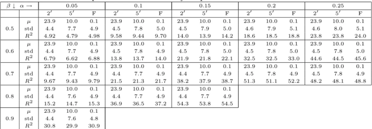
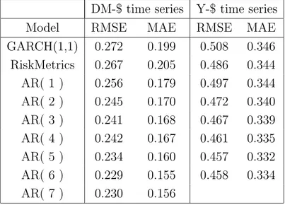
In the last twenty years, starting out from empirical investigations showing that volatility in financial time series is highly persistent with clustering phenomena, many models have been proposed to describe volatility evolution. The literature is now quite large with several specifications of auto-regressive models. Since empirical analysis have shown a high degree of intertemporal volatility persistence, then forecasting with an autoregressive specification should provide satisfactory results, but in many papers it has also been observed that fore-casting with GARCH models can be extremely unsatisfactory when the daily volatility is measured ex post by the squared (daily) return, see Andersen and Bollerslev (1998a); An-dersen et al. (1999); Figlewski (1997); Pagan and Schwert (1990). AnAn-dersen and Bollerslev (1998a) suggest that the main motivation of this failure is that the squared daily return is a very noisy estimator of volatility. Monte Carlo experiments of diffusion processes, whose parameters have been estimated on exchange rate time series (DM-$ and Yen-$), show that the noise of the high frequency volatility estimator is much smaller than that of the daily squared return. Then, they show as the forecasting performance of a GARCH(1,1) model is improved when the daily volatility (integrated volatility) is measured by means of the cu-mulative squared intraday returns. On this topic see also Barndorff-Nielsen and Shephard (2002a,b).
In this Chapter we address volatility estimation and forecasting in a GARCH setting with high frequency data by applying the algorithm described in Chapter 2 to compute the volatil-ity of a diffusion process. This method is based on Fourier analysis techniques (hereafter Fourier method). The volatility of a diffusion process is defined as the limit of its quadratic variation. This definition motivates standard volatility estimation methods based on a differ-entiation procedure: equation (1.11) of a process with a given frequency (day, week, month) is taken as a volatility estimate, see e.g. French et al. (1987). Extending this technique to intraday data presents some drawbacks due to the peculiar structure of high frequency data. For example, tick-by-tick data are not equally spaced. In the above cited papers an equally spaced time series for intraday returns is constructed by linearly interpolating logarithmic midpoints of bid-ask adjacent quotes or by taking the last quote before a given reference time (henceforth called imputation method). This procedure induces some distortions in the analysis, e.g. it may generate spurious returns autocorrelation, and it reduces the number of observations. The method adopted in this Chapter avoids these problems; it is based on integration of the time series, and it employs all the (irregularly spaced) observations. To compute integrals, we assume the price to be piecewise constant, i.e. the price is constant between two subsequent observations.
Volatility computation by using all the data with the Fourier method should then be more precise. We illustrate this fact through Monte Carlo simulations of a continuous-time GARCH(1,1) model with the parameters estimated in Andersen and Bollerslev (1998a). We also extend the simulation framework to representative models belonging to the SR-SARV(1) class (Andersen, 1994; Meddahi and Renault, 2004; Fleming and Kirby, 2003), which includes GARCH(1,1) as a particular case. We show that, in some settings, the vari-ance of our integrated volatility estimator is smaller than that of the cumulative squared intraday returns. Moreover, the precision of the cumulative squared intraday returns in measuring volatility depends on the procedure employed to build an equally spaced time se-ries. Linear interpolation causes a downward bias which increases with sampling frequency. The imputation method is immune from these drawbacks. When implementing the Fourier method with linearly interpolated observations instead of assuming the price to be piecewise constant, a strong downward bias arises as well.
Through Monte Carlo simulations, we show that, by measuring integrated volatility accord-ing to the Fourier method, the forecastaccord-ing performance of the GARCH(1,1) model, and other models belonging to the SR-SARV(1) class, is better than that obtained by computing volatility according to the cumulative squared intraday returns.
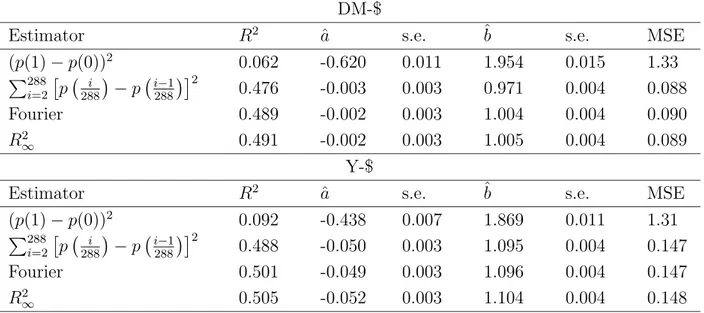
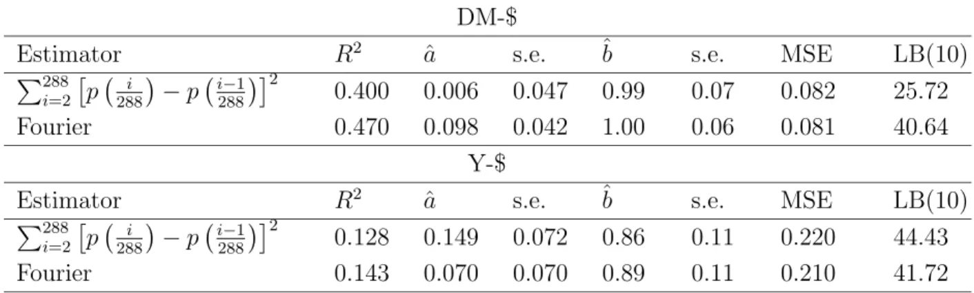
These results are confirmed when the method is applied to compute volatility of exchange rate high frequency time series. We apply the Fourier method to the evaluation of the
forecasting performance of the daily GARCH model and of the intraday GARCH model, as in Andersen et al. (1999). For both the time series considered, the GARCH model forecasts are evaluated to be better if the Fourier method is employed as a volatility estimate instead of the cumulative squared intraday returns.
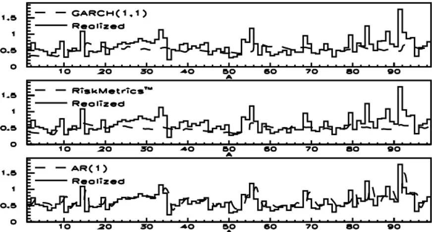
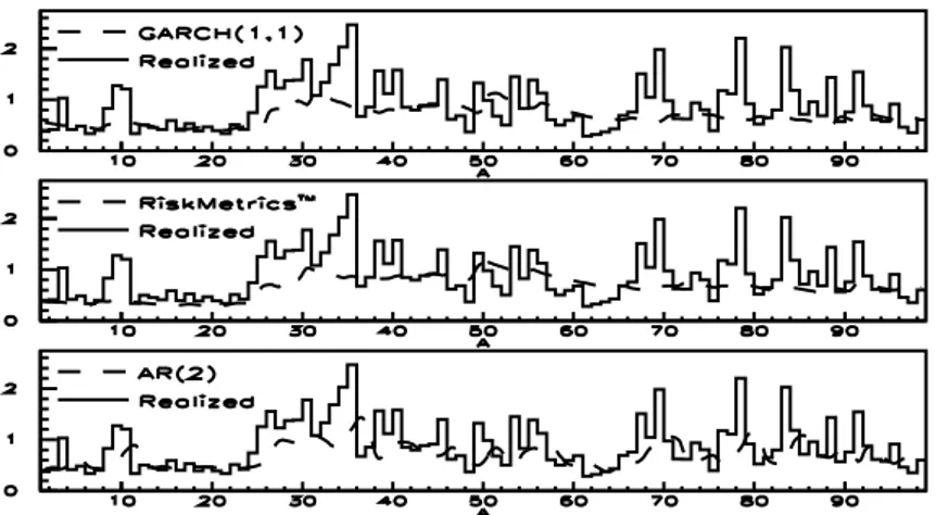
We then turn to directly modeling volatility measures. A good forecasting model for daily integrated volatility is crucial for VaR estimates. Traditional models regard volatility as a latent factor; here we model it as an observable quantity through an AR(n) model esti-mated by ordinary least squares. In spite of its simplicity, this model performs better than traditional models (GARCH(1,1) and Riskmetrics).
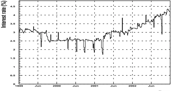
Finally we investigate the relationship between market activity and volatility in the Italian interbank overnight market. The interesting point is that this market is almost free of information asymmetry-heterogeneity. As a matter of fact, the overnight interest rate market is affected by liquidity conditions and by European Central Bank decisions, hence it is almost impossible for a bank to detain private information on them. Banks trade for pure hedging reasons. We show that definitely the number of contracts, and not trading volume, is associated with interest rate volatility. Our results confirm that liquidity management is the driving force of interest rate movements.
This Chapter is organized as follows. Section 3.2 describes the Monte Carlo experiments and assesses the performance of the Fourier method in measuring and forecasting volatility of simulated data. In Section 3.3 we turn to the analysis of foreign exchange rate data. Section 3.4 describes an application to Value at Risk measurement. In Section 3.5 we analyze the interest rate and volatility dynamics of the Italian money market. Section 3.6 concludes.
3.2
Monte Carlo experiments
In Barucci et al. (2000) we tested the Fourier method on equally spaced data. Monte Carlo experiments simulating a diffusion process with constant volatility showed that the method allows to consistently estimate volatility in a univariate setting and cross-volatilities in a mul-tivariate setting. The precision of the estimate is similar to that of classical methods. When applied to the daily time series of the Dow Jones Industrial and Dow Jones Transporta-tion Index, the Fourier method replicates the volatility estimates obtained by the classical method. Then there is no difference between the Fourier method and classical methods on equally spaced data.