2015
Publication Year
2021-01-19T10:14:34Z
Acceptance in OA@INAF
ARGO-YBJ Observation of the Large-scale Cosmic Ray Anisotropy During the
Solar Minimum between Cycles 23 and 24
Title
Bartoli, B.; Bernardini, P.; Bi, X. J.; Cao, Z.; Catalanotti, S.; et al.
Authors
10.1088/0004-637X/809/1/90
DOI
http://hdl.handle.net/20.500.12386/29835
Handle
THE ASTROPHYSICAL JOURNAL
Journal
809
ARGO-YBJ OBSERVATION OF THE LARGE-SCALE COSMIC RAY ANISOTROPY DURING THE
SOLAR MINIMUM BETWEEN CYCLES 23 AND 24
B. Bartoli1,2, P. Bernardini3,4, X. J. Bi5, Z. Cao5, S. Catalanotti1,2, S. Z. Chen5, T. L. Chen6, S. W. Cui7, B. Z. Dai8, A. D’Amone3,4, Danzengluobu6, I. De Mitri3,4, B. D’Ettorre Piazzoli1,2, T. Di Girolamo1,2, G. Di Sciascio9, C. F. Feng10,
Zhaoyang Feng5, Zhenyong Feng11, W. Gao7, Q. B. Gou5, Y. Q. Guo5, H. H. He5, Haibing Hu6, Hongbo Hu5, M. Iacovacci1,2, R. Iuppa9,12, H. Y. Jia11, Labaciren6, H. J. Li6, C. Liu5, J. Liu8, M. Y. Liu6, H. Lu5, L. L. Ma5, X. H. Ma5,
G. Mancarella3,4, S. M. Mari13,14, G. Marsella3,4, S. Mastroianni2, P. Montini9, C. C. Ning6, L. Perrone3,4, P. Pistilli13,14, P. Salvini15, R. Santonico9,12, P. R. Shen5, X. D. Sheng5, F. Shi5, A. Surdo4, Y. H. Tan5, P. Vallania16,17,
S. Vernetto16,17, C. Vigorito17,18, H. Wang5, C. Y. Wu5, H. R. Wu5, L. Xue10, Q. Y. Yang8, X. C. Yang8, Z. G. Yao5, A. F. Yuan6, M. Zha5, H. M. Zhang5, L. Zhang8, X. Y. Zhang10, Y. Zhang5, J. Zhao5, Zhaxiciren6, Zhaxisangzhu6,
X. X. Zhou11, F. R. Zhu11, and Q. Q. Zhu5 (The ARGO-YBJ Collaboration)
1
Dipartimento di Fisica dell’Università di Napoli “Federico II”, Complesso Universitario di Monte Sant’Angelo, via Cinthia, I-80126 Napoli, Italy 2Istituto Nazionale di Fisica Nucleare, Sezione di Napoli, Complesso Universitario di Monte Sant’Angelo, via Cinthia, I-80126 Napoli, Italy
3
Dipartimento Matematica e Fisica”Ennio De Giorgi”, Università del Salento, via per Arnesano, I-73100 Lecce, Italy 4
Istituto Nazionale di Fisica Nucleare, Sezione di Lecce, via per Arnesano, I-73100 Lecce, Italy 5
Key Laboratory of Particle Astrophysics, Institute of High Energy Physics, Chinese Academy of Sciences, P.O. Box 918, 100049 Beijing, P.R. China 6
Tibet University, 850000 Lhasa, Xizang, P.R. China 7
Hebei Normal University, 050024, Shijiazhuang Hebei, P.R. China;[email protected]
8
Yunnan University, 2 North Cuihu Road, 650091 Kunming, Yunnan, P.R. China
9Istituto Nazionale di Fisica Nucleare, Sezione di Roma Tor Vergata, via della Ricerca Scientifica 1, I-00133 Roma, Italy 10
Shandong University, 250100 Jinan, Shandong, P.R. China 11
Southwest Jiaotong University, 610031 Chengdu, Sichuan, P.R. China 12
Dipartimento di Fisica dell’Università di Roma “Tor Vergata”, via della Ricerca Scientifica 1, I-00133 Roma, Italy 13Dipartimento di Fisica dell’Università “Roma Tre”, via della Vasca Navale 84, I-00146 Roma, Italy 14
Istituto Nazionale di Fisica Nucleare, Sezione di Roma Tre, via della Vasca Navale 84, I-00146 Roma, Italy 15
Istituto Nazionale di Fisica Nucleare, Sezione di Pavia, via Bassi 6, I-27100 Pavia, Italy 16
Osservatorio Astrofisico di Torino dell’Istituto Nazionale di Astrofisica, via P. Giuria 1, I-10125 Torino, Italy 17
Istituto Nazionale di Fisica Nucleare, Sezione di Torino, via P. Giuria 1, I-10125 Torino, Italy 18
Dipartimento di Fisica dell’Università di Torino, via P. Giuria 1, I-10125 Torino, Italy Received 2015 May 29; accepted 2015 July 8; published 2015 August 12
ABSTRACT
This paper reports on the measurement of the large-scale anisotropy in the distribution of cosmic-ray arrival directions using the data collected by the air shower detector ARGO-YBJ from 2008 January to 2009 December, during the minimum of solar activity between cycles 23 and 24. In this period, more than 2× 10¹¹showers were recorded with energies between ∼1 and 30 TeV. The observed two-dimensional distribution of cosmic rays is characterized by two wide regions of excess and deficit, respectively, both of relative intensity ∼10−3with respect to a uniform flux, superimposed on smaller size structures. The harmonic analysis shows that the large-scale cosmic-ray relative intensity as a function of R.A. can be described by thefirst and second terms of a Fouries series. The high event statistics allow the study of the energy dependence of the anistropy, showing that the amplitude increases with energy, with a maximum intensity at∼10 TeV, and then decreases while the phase slowly shifts toward lower values of R.A. with increasing energy. The ARGO-YBJ data provide accurate observations over more than a decade of energy around this feature of the anisotropy spectrum.
Key words: cosmic rays– methods: data analysis – methods: observational
1. INTRODUCTION
The first observations showing that the arrival directions of very high energy cosmic rays (VHE CRs, E>100 GeV) are not isotropically distributed were performed in 1932, soon after the discovery of CRs. However, it was not until the 1950s that underground and surface detectors could provide clear evidence of sidereal anisotropy, with an intensity of 10−4−10−3 with respect to the isotropic background. The detectors measured the anisotropy as a variation of the cosmic-rayflux over the sidereal day and, based on harmonic analysis, the data from different experiments were compared in terms of the amplitudes and phases of the lowest-order harmonics.
In 1998, by combining the data from different experiments operating in the primary energy range ∼0.1–10 TeV and
located in the northern and southern hemispheres, two structures were recognized: an excess close to the direction of the heliotail(which has since been referred to as the “tail-in” excess) and a broad deficit in the direction of the Galactic North Pole, which authors thought originated from a poloidal, cone-shaped component of the galactic magnetic field (since then, named the“loss-cone”; Nagashima et al. 1998).
In the last decade, ground-based and underground/under-ice experiments with great statistics and good angular resolution have provided two-dimensional representations of the CR arrival directions, allowing for detailed morphological studies of the anisotropy structures. The new data concern both the northern hemisphere(Super Kamiokande, Tibet ASγ, Milagro, and ARGO-YBJ experiments) and the southern hemisphere
(the IceCube and IceTop experiments; Amenomori et al.2006; Guillian et al. 2007; Abdo et al. 2009; Zhang 2009; Abbasi et al. 2010, 2011, 2012; Aartsen et al. 2013). Although no systematic attempt has been made to merge all of the data to obtain a full-sky map of CRs, observations clearly depict a common large-scale structure in the arrival direction distribu-tion of CRs with energy less than 100 TeV. Dipole and quadrupole components mostly contribute to the“tail-in” (R.A. ∼50°–130°) and the “loss-cone” (R.A. ∼160°–240°). Narrower and less intense regions were also detected by the most sensitive experiments (Abdo et al. 2008; Abbasi et al. 2011; Bartoli et al.2013; Abeysekara et al.2014).
Of particular importance are the results at higher energies from EAS-TOP (Aglietta et al. 2009), IceCube (Abbasi et al.2012), and IceTop (Aartsen et al.2013) that have revealed a completely different scenario: a strong deficit at R.A. around 80° (relative intensity 2 × 10⁻³and size about 35°), at energies of∼400 TeV and ∼2 PeV, respectively, which is consistent with an abrupt phase variation of the first harmonics by ∼10 hr of sidereal time at energy above∼400 TeV.
Concerning the energy dependence of the observed aniso-tropy, the intensity shows a tendency to increase from 0.1 to 10 TeV, whereas the phase slowly shifts a few hours over the same energy interval. The results from Amenomori et al. (2006) showed a progressively smaller amplitude between 10 and 100 TeV. The Kascade collaboration did not detect any signal above 700 TeV(Antoni et al.2004), whereas EAS-TOP, IceCube, and IceTop detected modulations of increasing intensity above 400 TeV, accompanied by the above cited phase flip at ∼400 TeV (Aglietta et al. 2009; Abbasi et al.2012; Aartsen et al.2013).
The temporal behavior of the anisotropy is more contro-versial. While Milagro reported a steady increase of the intensity at a median energy of about 6 TeV from 2000 to 2007 (corresponding to a decrease of the solar activity; Abdo et al. 2009), the Tibet ASγ experiment did not observe any significant difference in the anisotropy intensity at ∼5 TeV for nine years of data from 1999 to 2008 (Amenomori et al. 2010, 2012). On the other hand, a weak correlation between the anisotropy amplitude at an energy of ∼0.6 TeV and the solar activity has been found in a 22 year muon data set (Munakata et al.2010).
A number of explanations for the CR anisotropy have been proposed. The ingredients for a model are CR production, acceleration, and propagation, which are considered together or independent of each other. The effect may simply relate to the uneven distribution of CR sources in the Galaxy or reflect propagation features that are not yet understood. The Galactic magnetic field and the local magnetic field, mostly in the heliosphere, likely play a major role in this area. If the heliosphere is one of the causes of the observed CR anisotropy, then one could expect a time variation for the effect related to the solar cycle.
Additionally, Compton and Getting predicted a dipolar anisotropy(not yet observed in sidereal time) due to the motion of the observer relative to the CR plasma. Assuming that CRs do not co-rotate with the Galaxy (Compton & Getting 1935), there would be an excess of CR intensity from the direction of motion of the solar system, while a deficit would appear in the opposite direction. Because of its purely kinematic origin, the Compton–Getting effect (CGE) is independent of the CR primary energy.
The recent works of Zhang et al.(2014) and Schwadron et al. (2014) discussed the local origin model of the anisotropies, while Qu et al.(2012) proposed a global galactic “CR Stream” model to understand the observation of the major anisotropic components in the solar vicinity. Some works focus on smaller-scale anisotropies, such as those observed by Milagro(Abdo et al.2008) and ARGO-YBJ (Bartoli et al.2013), and attempt to explain that the excess could be related to the Geminga pulsar as a local cosmic-ray source(Salvati & Sacco2010), or could be due to the magnetic mirror effect on CRs from a local source (Drury & Aharonian 2008). Many related studies are ongoing. However, a generally accepted theory capable of explaining all of the observations does not yet exist, and more data are necessary to provide solid ground for afirm theory.
This paper reports on observations of the large-scale anisotropy created by the air shower detector ARGO-YBJ from 2008 January to 2009 December, during the minimum of solar activity between cycles 23 and 24. ARGO-YBJ was equipped with a full-coverage “carpet” of particle detectors, a solution which significantly lowers the primary energy thresh-old and provides a high trigger rate. These features allowed for the accurate investigation of the CR anisotropy over the energy range∼1–30 TeV. The choice of limiting this work to the solar minimum period was made to reduce any possible influence of solar activity on the arrival distribution of cosmic rays. A study of the behavior of the anisotropy during the years of increasing solar activity of cycle 24 is deferred to a future publication.
In this article, the experiment layout and the detector performance are reported in Section 2. Section 3 contains a description of the analysis technique. Section 4 reports the results in terms of two-dimensionl maps and harmonic analysis in sidereal time. The energy dependence of the anisotropy is described and systematic uncertainties are discussed. A summary concludes the paper in the last section.
2. THE ARGO-YBJ EXPERIMENT
The ARGO-YBJ experiment is a full-coverage air shower detector located at the Yangbajing Cosmic Ray Laboratory (Tibet, P.R. China, longitude 90°. 5 east, latitude 30°. 1 north) at an altitude of 4300 m above the sea level, devoted to gamma-ray astronomy above ∼300 GeV and cosmic-ray studies above∼1 TeV.
The detector consists of a ∼74 × 78 m2 carpet made of a single layer of Resistive Plate Chambers (RPCs) with ∼92% active area, sorrounded by a partially instrumented (∼20%) area up to ∼100 × 110 m2. The apparatus has a modular structure where the basic data acquisition element is a cluster (5.7 × 7.6 m2) made of 12 RPCs (2.85 × 1.23 m2). Each RPC is read by 80 strips of 6.75× 61.8 cm2 (the spatial pixels), logically organized into 10 independent pads of 55.6× 61.8 cm2which are individually acquired and represent the time pixels of the detector(Aiellia et al.2006). To extend the dynamical range up to PeV energies, each RPC is equipped with two large pads(139 × 123 cm2) to collect the total charge developed by the particles hitting the detector. The full experiment is made of 153 clusters (18360 pads), for a total active surface of∼6600 m2.
ARGO-YBJ operates in two independent acquisition modes: the shower mode and the scaler mode. In shower mode, all showers with a number of hit pads Nhits 20 in the central carpet for a time window of 420 ns generate the trigger. The events collected in shower mode contain both digital and
analog information on the shower particles. In this analysis, we refer to the digital data recorded in shower mode.
The primary arrival direction is determined by fitting the arrival times of the shower front particles. The angular resolutions of cosmic-ray-induced showers have been checked using the Moon shadow(i.e., the shadow cast by the Moon on the cosmic-rayflux), observed by ARGO-YBJ with a statistical significance of ∼9 standard deviations per month. The shape of the shadow provided a measurement of the detector point-spread function, which has been found to agree with expectations. The angular resolution depends on Nhits(hereafter referred to as pad multiplicity) and varies from 0°. 3 for Nhits> 1000 to 1°. 8 for Nhits= 20–39 (Bartoli et al. 2011).
The pad multiplicity is used as an estimator of the primary energy. The relation between the primary energy and the pad multiplicity is given by Monte Carlo simulations. The reliability of the energy scale has been tested with the Moon shadow. Due to the geomagnetic field, cosmic rays are deflected according to their energy and the Moon shadow is shifted with respect to the Moon position by an amount depending on the primary energy. The westward shift of the shadow has been measured for different Nhits intervals and compared to simulations. We found that the total absolute energy scale error is less than 13% in the proton energy range ∼1–30 TeV, including uncertainties on the cosmic-ray ele-mental composition and the hadronic interaction model(Bartoli et al.2011).
3. DATA SELECTION AND ANALYSIS TECHNIQUE The full ARGO-YBJ detector was in stable data taking mode from 2007 November to 2013 February with a trigger rate of ∼3.5 kHz and an average duty cycle of ∼86%. For this analysis, the 2 × 10¹¹ events recorded in 2008–2009 were selected according to the following requirements:
1. more than 40 padsfired in the central carpet: Nhits 40; and 2. shower zenith angleθ < 45°.
About 3.6 × 10¹⁰ events survived the selection with arrival directions in the decl. band−10° < δ < +70°.
The isotropic CR background was estimated via the equi-zenith (EZ) angle method, wherein the expected distribution was fit to the experimental data by minimizing the residuals using an iteration technique (Amenomori et al. 2005a). This approach undoubtedly presents the advantage that it can account for effects caused by instrumental and environmental variations, such as changes in pressure or temperature. The method assumes that the events are uniformly distributed in azimuth for a given zenith angle bin, or at least that gradients are stable over a long time, as is the case for ARGO-YBJ(Li et al.2012; Bartoli et al.2014a).
Two sky maps are built with cells of 1° × 1° in R.A. α and decl.δ: the event map N(αi,δj) containing the detected events, and the background map Nb(a d containing the backgroundi, j) events as estimated by the EZ method. The maps are smoothed to increase the statistical significance, i.e., for each map bin, the events inside a circle of radius 5° around that bin are summed. Let Ii,jdenote the relative intensity in the sky cell (αi, δj), defined as the ratio of the number of detected events and the
estimated background events:
I N N , , . 1 i j i j i j , b
(
)
(
)
( ) a d a d =The statistical significance s of the excess (or deficit) of cosmic rays with respect to the expected background is given by s Ii j 1 2 I , i j, ( ) s =
-wheres is calculated from NIi j, (a d and Ni, j) b(a d takingi, j)
into account the number of bins used to evaluate the average background with the EZ method.
4. SIDEREAL ANISOTROPY
The significance map of the excesses obtained by ARGO-YBJ using the events with Nhits 40 is given in the first panel of Figure1, while the corresponding map showing the relative intensity of cosmic rays is reported in the second panel of the same figure. According to simulations (see next subsection), the median energy of the selected events is 1.3 TeV.
Two distinct large structures are visible: a complex excess region at R.A.= 50°–140° (the so called “tail-in” excess) and a broad deficit at R.A. = 150°–250° (the “loss-cone”). A small diffuse excess around R.A.= 310° and δ = 40° is also present with a significance of about 13 standard deviations, corre-sponding to the Cygnus region, mostly due to gamma-ray emission. The Cygnus region hosts a number of gamma-ray sources, plus an extended emission region detected by Fermi-LAT(Nolan et al.2012) and ARGO-YBJ (Bartoli et al.2014b)
Figure 1. Upper panel: significance map of the cosmic-ray relative intensity in the equatorial coordinate system for events with Nhits 40. Medium panel: relative intensity map. Lower panel: relative intensity as a function of the R.A., integrated over the decl. The line represents the best-fit curve obtained with the harmonic analysis. The abscissa bars present the widths of bins and the ordinate small error bars represent statistical errors.
known as the “Cygnus Cocoon.” Since ARGO-YBJ cannot distinguish between cosmic-ray and gamma-ray showers, the map of Figure 1also contains some excess due to gamma-ray sources, like the Crab Nebula (R.A. = 83°. 6,δ = 22°. 0). The excesses due to gamma-ray sources have a relatively small statistical significance compared to that reported by ARGO-YBJ in gamma-ray studies(Bartoli et al.2014c,2015) because the analysis parameters here are not optimized for gamma-ray measurements and the smoothing angle is much larger than the angular resolution for gamma-rays. Since the excesses due to gamma-rays are highly localized, they do not alter the large-scale structure of the map.
The lower panel of Figure1shows the intensity as a function of the R.A., obtained by projecting the two-dimensional map on the R.A. axis, in bins of 15°, and averaging over the decl. values. Following the standard harmonic analysis procedure, we fit the projected intensity with the first two terms of the Fourier series: I A x A x 1 cos 2 360 cos 2 180 , 3 1 1 2 2
[
]
[
(
)
]
( ) ( ) p j p j = + -+-where x is the R.A.
The obtained best-fit amplitudes and phases of the two harmonics are A1 = (6.8 ± 0.06) × 10−4, A2 = (4.9 ± 0.06) × 10−4,φ1= (39.1 ± 0.46)°, and φ2= (100.9 ± 0.32)° with aχ2/degrees of freedom (dof) = 1273/20.
The given errors are purely statistical. The poorχ2/dof value is due to the simple fitting function, which is not able to describe the complex morphology of the map, in particular, the R.A. region from 50° to 140°. Indeed, the fit does not improve substantially even by adding a third harmonic. More detailed analysis of these structures and their energy dependence have been discussed in Bartoli et al. (2013). Despite the large χ2 value due to the small structures superimposed on the smoother modulation, the figure shows that the general shape of the anisotropy can be satisfactorily described with two harmonics. Our data, similar to previous measurements by other detectors, rule out the hypothesis that the sidereal CGE is the dominant anisotropy component. The CGE has a purely kinetic nature, and directly follows from the relative motion of the observer and the medium. If the velocityfield is uniform, then the intensity of the anisotropy depends on v( ) · , where v tt n ( ) is the velocity of the medium with respect to the observer and n is the observing direction. Assuming that cosmic rays do not co-rotate with the Galaxy(Amenomori et al.2006), taking into account the Sunʼs orbital speed (∼200 km s−1), the CG effect predicts a dipole anisotropy of amplitude ACG= 3.5 × 10⁻³, which is much larger than what we observe, with the maximum in the direction of the motion of the solar system around the Galactic Center, (i.e., R.A. = 315° and δ = 49°) and the minimum in the opposite direction; this is inconsistent with the position of the excess and deficit regions observed in our analysis.
4.1. Anisotropy Versus Energy
Recent and past observations of cosmic rays have shown that the anisotropy is energy dependent. Thanks to its high statistics, ARGO-YBJ can separately study the anisotropy in different energy ranges. We divided the data into seven subsets, according to the number offired pads: Nhits = 40–59, 60–99, 100–160, 160–300, 300–700, 700–1000, and Nhits 1000.
The median energy corresponding to the above intervals has been estimated by means of a Monte Carlo simulation. The showers were generated by the CORSIKA code v.6.502(Heck et al.1998) assuming a power-law spectrum with a differential index ofα = −2.63 (Bartoli et al.2014d) and a primary energy ranging from 10 GeV to 1 PeV. Hadronic interactions at high energies are treated with the QGSJET-II model, while the low energy interactions are treated with GHEISHA. A total of 2× 10⁸events were sampled in the zenith angle band from 0° to 70°. A GEANT4-based detector simulation code was used to determine the detector response(Guo et al. 2010). The events were then selected according to the cuts used in the analysis of real data, and divided into seven samples according to the number of hits recorded by the detector. According to the simulations, the primary median energy corresponding to the different Nhitsintervals are: 0.98, 1.65, 2.65, 4.21, 7.80, 13.6, and 29.1 TeV, respectively.
The left panel of Figure 2(a) shows the relative intensity maps for the seven Nhits intervals. Structures with complex morphologies are visible in all of the maps, changing shape with energy. It has to be noted, however, that the structures at decl. δ < 0° and δ > 60° observed in the maps with Nhits 700 are statistical fluctuations due to the limited statistics, as can be deduced from Figure 2(b), which shows the statistical significance of the same maps.
As for the total sky map, harmonic analysis has been performed for the seven Nhitsintervals using the projection of the two-dimensional maps onto the R.A. axis. The best-fit curves are shown in the right panel of Figure 2(c), while the obtained values of amplitudes and phases are summarized in Table1.
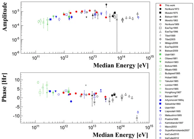
According to this analysis, the first harmonic amplitude steadily increases for energies from ∼1 to ∼10 TeV, after which it decreases. The amplitude almost doubles in less than one energy decade, then decreases to a smaller value for energies of ∼20–30 TeV. This trend is shown in the upper panel of Figure3, which reports the determined amplitudes as a function of the median primary energy, together with the results of other experiments covering the energy range ∼100 GeV–500 TeV (see Di Sciascio & Iuppa 2013 and references therein). All of the data agree on the existence of a maximum in intensity around∼10 TeV.
The lower panel of Figure 3 shows the phase of the first harmonics as a function of energy. The phase values found by ARGO-YBJ are consistent with the general trend of a slow phase decrease with energy up to about 400 TeV, when an abrupt change of phase occurs.
From Table1, one can see that the amplitude of the second harmonics is generally smaller than that of the first one. It shows a similar up-and-down trend with energy, but the percent variation is smaller: the amplitude increases by a factor∼1.5 in the energy interval 1–4 TeV, then decreases at higher energies. The trends of the amplitude and phase found in the harmonic analysis reflect the energy dependence of the intensity maps of Figure2. The absolute values of the minimum and maximum intensity increase with energy up to ∼10 TeV and decrease afterwards. At the same time, the regions of maximum and minimum intensity slightly shift toward lower R.A. values at the highest energies.
It is interesting to compare our data with the Tibet AS-γ array results given in Amenomori et al. (2012), which report the amplitude of the“loss-cone” deficit over 8 years, from 2000
to 2007, for three values of the primary median energy (4.4, 6.2, and 11 TeV), compared with a Milagro measurement at 6 TeV performed in about the same time interval. According to Tibet AS-γ data, the deficit amplitude (defined as the difference between unity and the relative intensity at the minimum of the best-fit curve of the harmonic analysis) is stable during the period under study with a value in the range∼0.0010–0.0013, while the Milagro data show a linear increase of the amplitude with time, going from∼0.0014 in 2001 to ∼0.0034 at the end of 2006. Our data, which closely follow the AS-γ and Milagro measurements in time, show a deficit amplitude in the range 0.0012–0.0016 for energies ∼4–14 TeV (see Figure 2(c)), in agreement with the Tibet results but not confirming the large increase observed by Milagro.
4.2. Systematic Uncertainties
Systematic errors in the sidereal analysis can be due to seasonal and diurnal effects, like atmospheric temperature and pressure variations that modify the cosmic-ray rate and the detector efficiency, and which do not completely cancel out even using full-year data. Considering the small amplitude of the anisotropy, systematics must be carefully evaluated and taken under control.
A standard test to verify the absence of solar effects in sidereal measurements is the harmonic analysis in anti-sidereal time. The anti-sidereal time is an artificial time which has 364.25 cycles per year, one day less than the number of days in a year of solar time, and two days less than the number of sidereal days. In principle, the harmonic analysis in
anti-sidereal time shouldfind no anisotropy at all, since no physical phenomena exist with such a periodicity. However, if some effect in solar time influences the sidereal distribution, it will also affect the anti-sidereal one. The anti-sidereal analysis is a valid method to estimate such systematics, and if needed, to correct them(Guillian et al.2007).
The results of the anti-sidereal analysis are reported in the last column of Table 1. The observed amplitudes provide a good estimate of the systematic uncertainty of the correspond-ing sidereal amplitudes for each Nhits interval. Since they are about 13% or less than the sidereal ones, a correction of the solar effects is not necessary for this analysis. For example, the upper panel of Figure4reports the anti-sidereal distribution for Nhits = 60–99. The lower panel shows that the effect of the correction on the sidereal analysis, performed according to the method described in Guillian et al.(2007), is negligible.
Further checks of the reliability of our data have been performed by exploiting the East–West method and the Compton Getting effect.
4.2.1. The East–West Method
Before the late 1990s, when experiments were not able to collect enough statistics to study the distribution of the CR arrival direction both in the R.A. and decl., measurements were performed by exploiting the “East–West” method (Aglietta et al. 2009; Bonino et al. 2011). This method is based on a differential approach: for each decl. belt, the difference of the event rate measured at+h and −h hour angle is considered. If this quantity is studied as a function of the local sidereal time,
Figure 2. (a) Cosmic-ray relative intensity maps for different Nhitsintervals; from top to bottom, Nhits= 40–59, 60–99, 100–159, 160–299, 300–699, 700–999, and Nhits 1000; (b) significance maps for the same Nhitsintervals;(c) projection of the two-dimensional intensity maps onto the R.A. axis; the curves are the best-fit functions obtained with the harmonic analysis. The error bars are statistical.
then the “derivative” of the sidereal anisotropy projection is obtained and a simple integration gives the sidereal anisotropy. This analysis is based on the difference between the event rates recorded simultaneously from different directions, and hence is free from systematics due to spurious rate variations. In the analysis presented here, h was calculated by averaging the hour angles of all of the events with a zenith angle less than 45°, and was found to be 18°. 6.
Due to the deep differences between the EZ and the East– West method, both in the approach and in handling data, a comparison between them provides a good estimate of systematic uncertainties. In Figure 5, the R.A. projections obtained with the EZ and the East–West methods are shown, for events with Nhits> 40. No significant differences are found between the two distributions and the agreement makes us confident on the reliability of the measurement.
4.2.2. Solar Compton Getting Effect
As explained previously, the CG effect was originally proposed as a prediction of a dipolar anisotropy which should be observed in sidereal time because of the motion of the solar system with respect to the CR medium. Such an anisotropy is not the only CG effect that can be investigated. In fact, the
Earth itself moves around the Sun and a CG effect should be observed in solar time. Like the sidereal CG effect, the solar CG effect can be predicted with a simple analytical model (Compton & Getting 1935). Given a power-law cosmic-ray spectrum, the fractional CR intensity variation I
I D is: I I v c 2 cos 4 (g ) a ( ) D = +
whereγ is the index of the spectrum, v is the Earthʼs velocity, c is the speed of light, and α is the angle between the arrival direction of cosmic rays and the direction of the detector motion, which changes continuously due to the Earth’s rotation and revolution. Assuming γ = 2.63 and v = 30 km s−1, by averaging the angle α over one year, the expected signal is a dipole anisotropy with an average amplitude of 3.82× 10⁻⁴at 6.0 hr of solar time.
Even if the observation of the solar CG effect is less important than the sidereal one(because there is no doubt that CRs do not co-rotate with the Earth around the Sun), nevertheless, it provides important indications as to the stability of the apparatus, and the agreement between observation and expectation would be a strong validator of the detector performance, as well as of the full chain of analysis.
Table 1
Results of the Harmonic Analysis for Seven NhitsIntervals
Em Harmonic Sidereal Time χ2/dof σstat Anti-sidereal
(TeV) Vectors Analysis Analysis
A1 6.1× 10⁻⁴ 0.1× 10⁻⁴ 0.8× 10⁻⁴ 0.98 φ1(°) 42.2 1.0 14.4 A2 4.4× 10⁻⁴ 321/20 0.1× 10⁻⁴ 0.2× 10⁻⁴ φ2(°) 101 0.7 0.5 A1 7.9× 10⁻⁴ 0.1× 10⁻⁴ 0.8× 10⁻⁴ 1.65 φ1(°) 31.7 1.1 11.8 A2 5.2× 10⁻⁴ 280/20 0.1× 10⁻⁴ 0.2× 10⁻⁴ φ2(°) 100 0.8 0.9 A1 9.8× 10⁻⁴ 0.2× 10⁻⁴ 0.8× 10⁻⁴ 2.65 φ1(°) 37.0 1.3 7.8 A2 5.4× 10⁻⁴ 86/20 0.2× 10⁻⁴ 0.6× 10⁻⁴ φ2(°) 100.7 1.2 0.1 A1 10.4× 10⁻⁴ 0.3× 10⁻⁴ 0.2× 10⁻⁴ 4.21 φ1(°) 28.4 1.5 7.1 A2 6.1× 10⁻⁴ 70/20 0.3× 10⁻⁴ 0.3× 10⁻⁴ φ2(°) 103.2 1.3 2.6 A1 11.6× 10⁻⁴ 0.4× 10⁻⁴ 0.4× 10⁻⁴ 7.80 φ1(°) 29.2 1.8 7.2 A2 5.2× 10⁻⁴ 53/20 0.4× 10⁻⁴ 0.6× 10⁻⁴ φ2(°) 102.2 2.0 2.6 A1 8.7× 10⁻⁴ 0.5× 10⁻⁴ 0.5× 10⁻⁴ 13.6 φ1(°) 36.9 3.6 2.7 A2 4.4× 10⁻⁴ 53/20 0.5× 10⁻⁴ 0.2× 10⁻⁴ φ2(°) 94.6 3.6 9.8 A1 3.8× 10⁻⁴ 0.5× 10⁻⁴ 0.4× 10⁻⁴ 29.1 φ1(°) 7.8 7.3 81.2 A2 3.9× 10⁻⁴ 46/20 0.5× 10⁻⁴ 0.3× 10⁻⁴ φ2(°) 88.7 3.6 12.5
Notes. Emis the median primary energy corresponding to each Nhitsinterval. The column“sidereal time analysis” reports the best-fit values of the harmonic analysis in sidereal time. The corresponding statistical errors are given in theσstatcolumm. The column“anti-sidereal analysis” reports the results in anti-sidereal time.
Since the effects of the Sun’s activity could influence the propagation of cosmic rays up to∼1–10 TeV, we study the CG signal using events of higher energy. Figure6reports the event distribution in solar time compared to that expected for showers with Nhits> 500, which correspond to a median primary energy of 13.7 TeV. The solar CG effect is clearly observed with an
Figure 3. Amplitude (upper panel) and phase (lower panel) of the first harmonic as a function of the energy, obtained by ARGO-YBJ, compared with the results of other experiments. (Sakakibara et al. 1973; Gombosi et al.1975; Alexeenko et al.1981; Cutler et al.1981; Lagage & Cesarsky 1983; Morello et al. 1983; Thambyaphillai1983; Nagashima et al.1985; Swinson & Nagashima1985; Andreyev et al.1987; Lee & Ng1987; Nagashima et al.1989; Kuznetsov1990; Ueno et al.1990; Cutler & Groom1991; Aglietta et al.1995,1996; Fenton et al.1995; Mori et al.1995; Munakata et al.1997,1999; Ambrosio et al.2003; Amenomori et al. 2005b; Guillian et al.2007; Abdo et al.2008,2009; Aglietta et al.2009; Alekseenko et al.2009; Abbasi et al.2010,2012.)
Figure 4. Upper panel: relative intensity of the anti-sidereal distribution for events with Nhits= 60–99. Lower panel: the corresponding sidereal distribution before and after the correction made with the anti-sidereal analysis.
Figure 5. Relative intensity of cosmic rays obtained using the Equi-Zenith method(dots) and the East–West method (triangles), together with the best-fit curve obtained with the harmonic analysis.
amplitude of (3.64 ± 0.36) × 10−4 and a phase of 6.67 ± 0.37 hr (χ2/dof = 34.5/16).
5. SUMMARY AND CONCLUSIONS
This paper reports on the measurement of the large-scale anisotropy by the ARGO-YBJ experiment in the energy range ∼1–30 TeV. The data collected in 2008 and 2009, during a phase of minimum solar activity, have been used to built a two-dimensional map of the CR intensity in the decl. band −10° < δ < +70°. Two large structures are observed, i.e., an excess region at R.A. = 50°–140° in the direction of the heliotail and a broad deficit at R.A. = 150°–250° in the direction of the Galactic North Pole(R.A. = 192°. 3,δ = 27°. 4). These observations are in fair agreement with previous results from other experiments using different techniques, supporting the robustness of the result. In particular, the amplitude of the deficit is consistent with that measured by the Tibet AS-γ array during the previous 8 years.
The high statistics of our sample allowed the detection of many structures of angular size as small as∼10°, superimposed on the largest structures. Even neglecting such small structures, the observed anisotropy is not a pure dipole and the harmonic analysis of the intensity distribution as a function of the R.A. shows that the data can be described by the first two components of a Fourier series, representing the diurnal and semidiurnal sidereal modulation. The amplitude of the first harmonic is about a factor of 1.5 larger than the second.
The energy dependence of the anisotropy has been studied building two-dimensional sky maps for seven different intervals of event multiplicity with median energies ranging from 1 to 30 TeV. The excess and deficit regions are observed with high significance. The data show that the absolute value of the intensity of both regions increases with energy up to ∼10 TeV, then decreases, while the positions of both the maximum and the minimum slightly shift toward smaller values of R.A. The similar energy dependence could suggest that the origin of the excess and deficit regions is the same.
The harmonic analysis shows that the amplitude of thefirst harmonic increases with energy and doubles in the range ∼1–10 TeV, then decreases. The position of maximum intensity is consistent with the data of other detectors working in different energy ranges. The general scenario is that thefirst harmonic amplitude increases by a factor of ∼5 in the energy range∼100 GeV–10 TeV, and then decreases until the energy
reaches ∼400 TeV where the phase abruptly changes. The phase observed by ARGO-YBJ is around 3 hr of sidereal time, consistent with the decrease trend observed in the 100 GeV– 300 TeV range. The second harmonic amplitude also shows similar behavior, but the variation is smaller.
In conclusion, the ARGO-YBJ data provide accurate observations in the energy range where the anisotropy reaches its maximum intensity, with a set of high statistics data covering more than one decade of energy around this feature. The reliability of the data and the analysis technique has been checked using the East–West method, which gives consistent results, and with the observation of the solar CG effect at energies above 10 TeV, where the Sun activity effects are expected to be negligible.
The origin of the observed anisotropy is still unknown. Galactic cosmic rays are believed to be accelerated by supernova blast waves and then trapped in the Galactic magnetic fields. Since the strength of the magnetic fields is supposed to be of the order of a few micro-Gauss, the gyro-radii of CRs of energy 1–10 TeV could be of the order of 10-2–
10-3pc, which is much smaller than the thickness of the
Galactic disk(∼200 pc). Hence, the motion of cosmic rays is expected to be randomized and the arrival direction highly isotropical. The observed small anisotropies are likely due to the superimposition of different components which operate at different scales. The distribution of sources, the irregularities of the magneticfield, in particular in the neighborhood of the Sun, likely contribute to some extent to shape the cosmic-ray spatial distribution. The heliosphere could contribute to model the anisotropy below 10 TeV with possible effects related to solar activity. All of these components can be disentangled in the future only with more precise measurements exploring in detail the angular structures and the evolution of cosmic-ray anisotropies over a wide energy range.
This work is supported in China by NSFC(No. 11375052, No. 10975046, No. 10120130794, No. 11165013), the Chinese Ministry of Science and Technology, the Chinese Academy of Sciences, and the Key Laboratory of Particle Astrophysics, CAS, and in Italy by the Istituto Nazionale di Fisica Nucleare (INFN). We also acknowledge essential support from W.Y. Chen, G. Yang, X. F. Yuan, C. Y. Zhao, R. Assiro, B. Biondo, S. Bricola, F. Budano, A. Corvaglia, B. D’Aquino, R. Esposito, A. Innocente, A. Mangano, E. Pastori, C. Pinto, E. Reali, F. Taurino, and A. Zerbini in the installation, debugging, and maintenance of the detector.
REFERENCES
Aartsen, M. G., Abbasi, R., Abdou, Y., et al. 2013,ApJ,765, 55 Abbasi, R., Abdou, Y., Abu-Zayyad, T., et al. 2010,ApJL,718, L194 Abbasi, R., Abdou, Y., Abu-Zayyad, T., et al. 2011,ApJ,740, 16 Abbasi, R., Abdou, Y., Abu-Zayyad, T., et al. 2012,ApJ,746, 33 Abdo, A. A., Allen, B., Aune, T., et al. 2008,PhRvL,101, 221101 Abdo, A. A., Allen, B., Aune, T., et al. 2009,ApJ,698, 2121 Abeysekara, A. U., Alfaro, R., Alvarez, C., et al. 2014,ApJ,796, 108 Aglietta, M., Alessandro, B., Antonioli, P., et al. 1995, in Proc. 24th ICRC,
4, 800
Aglietta, M., Alessandro, B., Antonioli, P., et al. 1996,ApJ,470, 501 Aglietta, M. V., Alekseenko, V., Alessandro, B., et al. 2009,ApJL,692, L130 Aiellia, G., Assirob, R., Baccic, C., et al. 2006,NIMPA,562, 92
Alekseenko, V. V., Cherniaev, A. B., Djappuev, D. D., et al. 2009, NuPhB, 196, 179
Alexeenko, V. V., Chudakov, E. A., Gulieva, N. E., & Sborshikov, G. V. 1981, in Proc. 17th ICRC, 2, 146
Ambrosio, M., Antolini, R., Baldini, A., et al. 2003,PhRvD,67, 042002 Figure 6. Projection of the event distribution in solar time for Nhits> 500. The
dotted line represents the expected Compton–Getting modulation. The abscissa bars present the width of bins and the ordinate errors are statistical.
Amenomori, M., Ayabe, S., Bi, X. J., et al. 2006,Sci,314, 439 Amenomori, M., Ayabe, S., Cui, S. W., et al. 2005a,ApJ,633, 1005 Amenomori, M., Ayabe, S., Cui, S. W., et al. 2005b,ApJL,626, L32 Amenomori, M., Bi, X. J., Chen, D., et al. 2010,ApJ,711, 119 Amenomori, M., Bi, X. J., Chen, D., et al. 2012,APh,36, 237
Andreyev, Y. M., Chudakov, A. E., Kozyarivsky, V. A., et al. 1987, in Proc. 20th ICRC, 2, 22
Antoni, T., Apel, W. D., Badea, A. F., et al. 2004,ApJ,604, 687 Bartoli, B., Bernardini, P., Bi, X. J., et al. 2011,PhRvD,84, 022003 Bartoli, B., Bernardini, P., Bi, X. J., et al. 2013,PhRvD,88, 082001 Bartoli, B., Bernardini, P., Bi, X. J., et al. 2014a,PhRvD,89, 052005 Bartoli, B., Bernardini, P., Bi, X. J., et al. 2014b,ApJ,790, 152 Bartoli, B., Bernardini, P., Bi, X. J., et al. 2014c,ApJ,779, 27 Bartoli, B., Bernardini, P., Bi, X. J., et al. 2014d,ChPhC,38, 045001 Bartoli, B., Bernardini, P., Bi, X. J., et al. 2015,ApJ,798, 119
Bonino, R., Alexeenko, V. V., Deligny, O., & Ghia, P. L. 2011,ApJ,738, 67 Compton, A. H., & Getting, I. A. 1935,PhRvL,47, 817
Cutler, D. J., Bergeson, H. E., Davies, J. F., & Groom, D. E. 1981, ApJ, 248, 1166
Cutler, D. J., & Groom, D. E. 1991,ApJ,376, 322
Di Sciascio, G., & Iuppa, R. 2013, in Homage to the Discovery of Cosmic Rays, the Meson-Muons and Solar Cosmic Rays(New York: Nova Science Publishers, Inc.) arXiv:1407.2144
Drury, L., & Aharonian, F. 2008,APh,29, 420
Fenton, K. B., Fenton, A. G., & Humble, J. E. 1995, in Proc. 24th ICRC, 4, 635 Gombosi, T., Kota, J., Somogyi, A. J., et al. 1975, in Proc. 14th ICRC, 2, 586 Guillian, G., Hosaka, J., Ishihara, K., et al. 2007,PhRvD,75, 062003 Guo, Y. Q., Zhang, X. Y., Zhang, J. L., et al. 2010,ChPhC,34, 555
Heck, D., Knapp, J., Capdevielle, J. N., et al. 1998, CORSIKA: A Monte Carlo Code to Simulate Extensive Air Showers, Forshungszentrum Karlsruhe, FZKA 6019
Kuznetsov, A. V. 1990, in Proc. 21st ICRC, 6, 372 Lagage, P. O., & Cesarsky, C. J. 1983, A&A,125, 249 Lee, Y. W., & Ng, L. K. 1987, in Proc. 20th ICRC, 2, 18
Li, T. L., Liu, M. Y., Cui, S. W., & Hou, Z. T. 2012,APh,39–40, 144 Morello, C., Navarra, G., & Vernetto, S. 1983, in Proc. 18th ICRC,
1, 137
Mori, S., Yasue, S., Munakata, K., et al. 1995, in Proc. 24th ICRC, 4, 648 Munakata, K., Hara, T., Yasue, S., et al. 1999,AdSpR,23, 611
Munakata, K., Kiuchi, T., Yasue, S., et al. 1997,PhRvD,56, 23 Munakata, K., Mizoguchi, Y., Kato, C., et al. 2010,ApJ,712, 1100 Nagashima, K., Fujimoto, K., & Jacklyn, R. M. 1998,JGR,103, 17429 Nagashima, K., Fujimoto, K., Sakakibara, S., et al. 1989,NCimC,12, 695 Nagashima, K., Sakakibara, S., Fenton, A. G., & Humble, J. E. 1985,P&SS,
33, 395
Nagashima, K., Ueno, H., Fujimoto, K., et al. 1975, Proc. 14th ICRC, 4, 1053 Nolan, P. L., Abdo, A. A., Ackermann, M., et al. 2012,ApJS,199, 31 Qu, X. B., Zhang, Y., Xue, L., et al. 2012,ApJL,750, L17
Sakakibara, S., et al. 1973, in Proc. 13th ICRC, 2, 1058 Salvati, M., & Sacco, B. 2010,A&A,513, A28
Schwadron, N. A., Adams, F. C., Christian, E. R., et al. 2014,Sci,343, 988 Swinson, D. B., & Nagashima, K. 1985,P&SS,33, 1069
Thambyaphillai, T. 1983, in Proc. 18th ICRC, 3, 383
Ueno, H., Fujii, Z., Yamada, T., et al. 1990, in Proc. 21st ICRC, 6, 361 Zhang, J. L., Zhang, Y., Cui, S. W., et al. 2009, in Proc. 31st ICRC Zhang, M., Zuo, P. B., & Pogorelov, N. 2014,ApJ,790, 5