Artificial Intelligent based
Multi Agent Control Systems
Federico Lisi
FACOLTÀ DI INGEGNERIA DELL’INFORMAZIONE,
INFORMATICA E STATISTICA
PhD Program in Automatica, Bioengineering and Operation
Research
CURRICULUM IN AUTOMATICA
Advisor
Chiar.mo Prof. Francesco Delli Priscoli
Candidate
Ing. Federico Lisi
DIAG - DIPARTIMENTO DI INGEGNERIA INFORMATICA,
AUTOMATICA E GESTIONALE ANTONIO RUBERTI
Declaration
I, Federico Lisi, hereby declare that this PhD thesis, titled "Artificial Intelligent based Multi Agent Control Systems (Sistemi di Controllo Multi Agent basati su tecniche di Intelligenza Artificiale)", and the work in it are my own. I confirm that:
1. this work has been done mainly during the research activities performed in my own PhD carrier at the University of Rome "La Sapienza".
2. some part of this PhD thesis was presented in MIUR project and H2020 project
3. some part of this PhD thesis are already presented, submitted and accepted in international publication for both Journal and Conference. 4. where I have consulted other published works they are always cited. 5. where I have quoted from the work of others, the source is always given
and, with the exception of such quotations, this thesis is entirely my own work
6. the co-authors of my published works are thanked in proper section of this PhD thesis
In faith,
Inscription
Fig. 1 Pale Blue Dot, Carl Segan
"We succeeded in taking that picture [from deep space], and, if you look at it, you see a dot. That’s here. That’s home. That’s us. On it, everyone you ever heard of, every human being who ever lived, lived out their lives. The aggregate of all our joys and sufferings, thousands of confident religions, ideologies and economic doctrines, every hunter and forager, every hero and coward, every creator and destroyer of civilizations, every king and peasant, every young couple in love, every hopeful child, every mother and father, every inventor and explorer, every teacher of morals, every corrupt politician, every superstar, every supreme leader, every saint and sinner in the history of our species, lived there on a mote of dust, suspended in a sunbeam.
blood spilled by all those generals and emperors so that in glory and in triumph they could become the momentary masters of a fraction of a dot. Think of the endless cruelties visited by the inhabitants of one corner of the dot on scarcely distinguishable inhabitants of some other corner of the dot. How frequent their misunderstandings, how eager they are to kill one another, how fervent their hatreds. Our posturings, our imagined self-importance, the delusion that we have some privileged position in the universe, are challenged by this point of pale light.
Our planet is a lonely speck in the great enveloping cosmic dark. In our obscurity – in all this vastness – there is no hint that help will come from elsewhere to save us from ourselves. It is up to us. It’s been said that as-tronomy is a humbling, and I might add, a character-building experience. To my mind, there is perhaps no better demonstration of the folly of human conceits than this distant image of our tiny world. To me, it underscores our responsibility to deal more kindly and compassionately with one another and to preserve and cherish that pale blue dot, the only home we’ve ever known." "Da questo distante punto di osservazione, la Terra può non sembrare di particolare interesse. Ma per noi, è diverso. Guardate ancora quel puntino. È qui. È casa. È noi. Su di esso, tutti coloro che amate, tutti coloro che conoscete, tutti coloro di cui avete mai sentito parlare, ogni essere umano che sia mai esistito, hanno vissuto la propria vita. L’insieme delle nostre gioie e dolori, migliaia di religioni, ideologie e dottrine economiche, così sicure di sé, ogni cacciatore e raccoglitore, ogni eroe e codardo, ogni creatore e distruttore di civiltà, ogni re e plebeo, ogni giovane coppia innamorata, ogni madre e padre, figlio speranzoso, inventore ed esploratore, ogni predicatore di moralità, ogni politico corrotto, ogni "superstar", ogni "comandante supremo", ogni santo e peccatore nella storia della nostra specie è vissuto lì, su un minuscolo granello di polvere sospeso in un raggio di sole. La Terra è un piccolissimo palco in una vasta arena cosmica.
Pensate ai fiumi di sangue versati da tutti quei generali e imperatori affinché, nella gloria e nel trionfo, potessero diventare per un momento padroni di una frazione di un puntino. Pensate alle crudeltà senza fine inflitte dagli abitanti di un angolo di questo pixel agli abitanti scarsamente distinguibili di qualche altro angolo, quanto frequenti le incomprensioni, quanto smaniosi di uccidersi a vicenda, quanto fervente il loro odio. Le nostre ostentazioni, la nostra
immagi-ix
naria autostima, l’illusione che noi abbiamo una qualche posizione privilegiata nell’Universo, sono messe in discussione da questo punto di luce pallida. Il nostro pianeta è un granellino solitario nel grande, avvolgente buio cosmico. Nella nostra oscurità, in tutta questa vastità, non c’è alcuna indicazione che possa giungere aiuto da qualche altra parte per salvarci da noi stessi.
La Terra è l’unico mondo conosciuto che possa ospitare la vita. Non c’è altro posto, per lo meno nel futuro prossimo, dove la nostra specie possa migrare. Visitare, sì. Colonizzare, non ancora. Che ci piaccia o meno, per il momento la Terra è dove ci giochiamo le nostre carte. È stato detto che l’astronomia è un’esperienza di umiltà e che forma il carattere. Non c’è forse migliore dimostrazione della follia delle vanità umane che questa distante immagine del nostro minuscolo mondo. Per me, sottolinea la nostra responsabilità di occuparci più gentilmente l’uno dell’altro, e di preservare e proteggere il pallido punto blu, l’unica casa che abbiamo mai conosciuto."
Acknowledgements
I would like to express my deepest gratitude to my PhD Supervisor, Professor Francesco Delli Priscoli, for believing in me and for being a working guide. I will always carry all his teachings with me.
I would like to thank Dr. Silvia Canale for having trained me professionally, for having teaching me how to work internationally, for helping me in the difficulty encountered during my work, and for being close to me until at the end of this trip.
I would like to thank Professor Antonio Pietrabissa, the nicest and most serious person I’ve ever met. I thank him for helping me in developing some part of this work, and for being a special working and life guide. A special thank to my friends and colleagues Raffaele Gambuti, Alessandro Giuseppi and Martina Panfili for the time spent together.
I would like to thank all my colleagues Vincezo Suraci, Alessandro Di Gior-gio, Letterio Zuccaro, Lorenzo Ricciardi Celsi, Federico Cimorelli, Francesco Liberati, Antonio Ornatelli and Andrea Tortorelli
Lastely, I would like to thank my parents for helping me during these years, I would like also thank my brother, and my grandparents.
This work was being possible also thanks to the love of my life, LARA.
Desidero esprimere la mia più profonda gratitudine al Professore Francesco Delli Priscoli, per aver creduto in me e per essere stato la guida durante lo svolgimento di questo lavoro. Porterò sempre con me tutti i suoi insegnamenti. Vorrei ringraziare la Dottoressa Silvia Canale per avermi formato professional-mente, per avermi insegnato come lavorare a livello internazionale, per avermi aiutato nella difficoltà durante il lavoro e per essermi stata vicino fino alla fine di questo viaggio.
Vorrei ringraziare il Professore Antonio Pietrabissa, la persona più bella e seria che abbia mai incontrato. Lo ringrazio per avermi aiutato nello sviluppo di una parte di questo lavoro e per essere stato una speciale guida di vita e di lavoro. Un ringraziamento speciale al miei amici e colleghi Raffaele Gambuti, Alessandro Giuseppi e Martina Panfili.
Vorrei ringraziare tutti i miei colleghi Vincezo Suraci, Alessandro Di Gior-gio, Letterio Zuccaro, Lorenzo Ricciardi Celsi, Federico Cimorelli, Francesco Liberati, Antonio Ornatelli e Andrea Tortorelli.
Infine, mi piacerebbe ringraziare i miei genitori per avermi aiutato in questi anni, grazie anche a mio fratello e ai miei nonni.
Abstract
Artificial Intelligence (AI) is a science that deals with the problem of having machines perform intelligent, complex, actions with the aim of helping the human being. It is then possible to assert that Artificial Intelligence permits to bring into machines, typical characteristics and abilities that were once limited to human intervention. In the field of AI there are several tasks that ideally could be delegated to machines, such as environment aware perception, visual perception and complex decisions in various field.
The recent research trends in this field have produced remarkable upgrades mainly on complex engineering systems such as multi-agent systems, networked systems, manufacturing, vehicular and transportation systems, health care; in fact, a portion of the mentioned engineering system is discussed in this PhD thesis, as most of them are typical field of application for traditional control systems.
The main purpose if this work is to present my recent research activities in the field of complex systems, bringing artificial intelligent methodologies in different environment such as in telecommunication networks, transportation systems and health care for Personalized Medicine.
The designed and developed approaches in the field of telecommunication net-works is presented in Chapter 2, where a multi-agent reinforcement learning algorithm was designed to implement a model-free control approach in order to regulate and improve the level of satisfaction of the users, while the research activities in the field of transportation systems are presented at the end of Chapter 2 and in Chapter 3, where two approaches regarding a Reinforcement Learning algorithm and a Deep Learning algorithm were designed and developed to cope with tailored travels and automatic identification of transportation moralities. Finally, the research activities performed in the field of Personalized Medicine have been presented in Chapter 4 where a Deep Learning and Model Predictive control based approach are presented to address the problem of controlling biological factors in diabetic patients.
Le metodologie di Intelligenza Artificiale (AI) si occupano della possibilità di rendere le macchine in grado di compiere azioni intelligenti con lo scopo di aiutare l’essere umano; quindi è possibile affermare che l’Intelligenza Artificiale consente di portare all’interno delle macchine, caratteristiche tipiche considerate come caratteristiche umane.
Nello spazio dell’Intelligenza Artificiale ci sono molti compiti che potrebbero essere richiesti alla macchina come la percezione dell’ambiente, la percezione visiva, decisioni complesse.
La recente evoluzione in questo campo ha prodotto notevoli scoperte, princi-palmente in sistemi ingegneristici come sistemi multi-agente, sistemi in rete, impianti, sistemi veicolari, sistemi sanitari; infatti una parte dei suddetti sistemi di ingegneria è presente in questa tesi di dottorato.
Lo scopo principale di questo lavoro è presentare le mie recenti attività di ricerca nel campo di sistemi complessi che portano le metodologie di intelligenza artifi-ciale ad essere applicati in diversi ambienti, come nelle reti di telecomunicazione, nei sistemi di trasporto e nei sistemi sanitari per la Medicina Personalizzata. Gli approcci progettati e sviluppati nel campo delle reti di telecomunicazione sono presentati nel Capitolo 2, dove un algoritmo di Multi Agent Reinforcement Learning è stato progettato per implementare un approccio model-free al fine di controllare e aumentare il livello di soddisfazione degli utenti; le attività di ricerca nel campo dei sistemi di trasporto sono presentate alla fine del capitolo 2 e nel capitolo 3, in cui i due approcci riguardanti un algoritmo di Reinforcement Learning e un algoritmo di Deep Learning sono stati progettati e sviluppati per far fronte a soluzioni di viaggio personalizzate e all’identificazione automatica dei mezzi trasporto; le ricerche svolte nel campo della Medicina Personalizzata sono state presentate nel Capitolo 4 dove è stato presentato un approccio basato sul controllo Deep Learning e Model Predictive Control per affrontare il problema del controllo dei fattori biologici nei pazienti diabetici.
Table of contents
List of figures xvii
List of tables xix
1 Introduction 1
2 Reinforcement Learning based Multi Agent Control Systems 7
2.1 Reinforcement Learning . . . 8
2.2 Multi Agent Reinforcement Learning . . . 11
2.2.1 Matrix Games . . . 11
2.2.2 Nash Equilibrium . . . 13
2.2.3 Stochastic Game . . . 14
2.2.4 Nash Q-Learning . . . 15
2.2.5 Friend-or-Foe Q-Learning . . . 18
2.3 Multi Agent Control Systems applied to telecommunication networks . . . 21
2.3.1 QoE Controller . . . 22
2.3.2 Proposed Heuristic MARL-Q based (H-MARL-Q) algo-rithm . . . 28
2.3.3 H-MARL-Q algorithm simulation . . . 32
2.4 RL Control approach applied to transportation system . . . 41
2.4.1 Reference scenario . . . 44
2.4.2 Extended Intelligent Transportation System . . . 46
2.4.3 Data Driven User Profiling . . . 50
2.4.4 User Centric Control System . . . 54
2.4.5 Adaptive Rank and Results . . . 61
3 Deep Learning based Intelligent Transportation System 69
3.1 Introduction . . . 69
3.2 Deep Learning . . . 72
3.2.1 Perceptron . . . 73
3.2.2 Artificial Neural Networks . . . 75
3.2.3 Deep Recurrent Neural Networks . . . 77
3.2.4 Deep Convolutional Neural Networks . . . 81
3.2.5 Deep AutoEncoders . . . 83
3.3 Transportation Mode Recognition Problem . . . 85
3.3.1 Problem Statement . . . 87
3.3.2 Data Collection . . . 88
3.3.3 Features Extraction approach . . . 90
3.3.4 Raw Data approach . . . 91
3.3.5 Deep Recurrent Neural Network . . . 92
3.3.6 Deep Convolution Neural Network . . . 93
3.3.7 Real Time Recognition . . . 95
3.3.8 Results . . . 95
3.4 Traffic Control based Future Works . . . 99
4 Deep Model Predictive Control based techniques 101 4.1 Blood Glucose Level Control . . . 102
4.2 Model Predictive Control . . . 103
4.3 Deep Model Predictive Control . . . 106
4.4 DeepMPC Artificial Pancreas . . . 108
4.5 Results . . . 114
4.6 Future Work . . . 116
5 Conclusion 119
List of figures
1 PaleBlue . . . vii
2.1 Grid Game . . . 16
2.2 Nash Strategy . . . 16
2.3 Example Network . . . 33
2.4 QoE Average absolute error for 100 agents . . . 37
2.5 QoE Average absolute error for 1000 agents . . . 38
2.6 QoE Standard Deviation for 100 agents . . . 38
2.7 QoE Standard Deviation for 1000 agents . . . 39
2.8 Average absolute QoE error . . . 39
2.9 Intelligent Transportation System . . . 42
2.10 Extended Intelligent Transportation System . . . 43
2.11 Human Machine Interaction with learning system . . . 55
2.12 Control Scheme for Intelligent Transportation System . . . 56
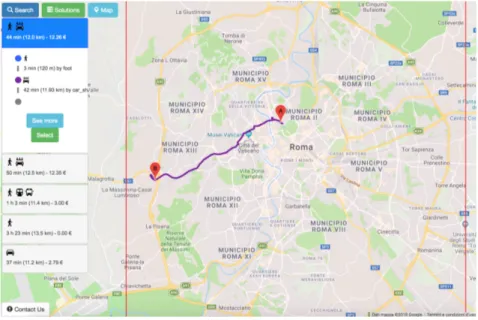
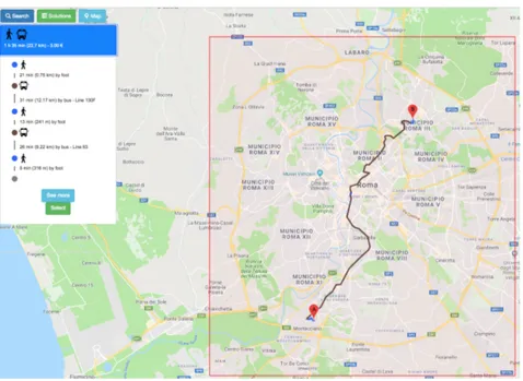
2.13 Travel Solution Example . . . 63
2.14 Travel Solutions Example . . . 63
2.15 Travel Solutions Example . . . 65
2.16 Travel Solutions Example . . . 65
2.17 Travel Solutions Example . . . 66
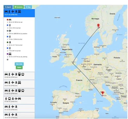
2.18 Tailored Solution . . . 67
3.1 Single Unit - Perceptron . . . 74
3.2 Artificial Neural Network architecture . . . 76
3.3 Deep FeedForward Neural Network architecture . . . 77
3.4 Simple Recurrent Neural Network architecture . . . 78
3.5 LSTM architecture . . . 79
3.6 Bidirection LSTM architecture . . . 81
3.7 Deep Convolutional Neural Network architecture . . . 82
3.9 Deep AutoEncoders architecture . . . 84
3.10 Transportation Mode Recognition . . . 88
3.11 Resultant acceleration over 8 seconds . . . 89
3.12 Features Extraction based approach . . . 90
3.13 Features Extraction based classification . . . 90
3.14 Raw Data approach . . . 91
3.15 Raw Data Classification . . . 91
3.16 Deep Recurrent Neural Network . . . 92
3.17 Deep Convolutional Neural Network . . . 94
3.18 Example of Motion Flow . . . 99
4.1 Deep Model Predictive Control . . . 107
4.2 DeepMPC novel approach . . . 111
4.3 Predicted and Target glycemic level . . . 115
4.4 Deep MPC Control . . . 117
List of tables
2.1 Representation of the reduced joint action space for N=4 and S=3 32
2.2 Data Record . . . 51
3.1 Confusion Matrix for Deep Recurrent Neural Network . . . 96
3.2 Confusion Matrix for Deep Convolutional Neural Network . . . 97
3.3 Average Total Performances for Deep Recurrent Neural Network 97 3.4 Average Total Performances for Deep Convolutional Neural Net-work . . . 97
3.5 Real Environment Performances for Deep Recurrent Neural Network . . . 98
3.6 Real Environment Performances for Deep Convolutional Neural Network . . . 98
4.1 Partial content of the dataset . . . 112
4.2 Variable Meals for specific patients . . . 113
4.3 On-line diabetic patient state . . . 113
4.4 Glycemic index over the predicted periods . . . 113
4.5 Glycemic index over the predicted periods . . . 114
Chapter 1
Introduction
Artificial Intelligence (AI) methodologies deal with the possibility to make machines able to perform intelligent actions with the aim of helping the human being; then is possible to assert that Artificial Intelligence permits to bring into the machine, typical characteristics considered as humans. In the AI space there are a lot of tasks that could be demanded to machine such as environment aware perception, visual perception, complex decisions.
AI is experiencing a moment of great interest in the scientific community, as never before, thanks above all to the current computation power of the modern computers. Currently, several different research activities are really active to bring AI practically everywhere, and some industrial companies are ready to in-stall working AI tools into the services and things. Bringing intelligence within things means not only have machines/computers with relevant computational power but also endow the machines with reasoning capabilities. The recent evolving in this field has produced remarkable upgrades mainly on engineering systems such as multi-agent systems, networked systems, manufacturing sys-tems, vehicular syssys-tems, health care syssys-tems, etc... .
The main scope of my recent research activities is a tentative approach to use intelligent control [1] [77], a data driven control framework [47] [102], which uses typical artificial intelligence methodologies, such as Neural Network [110], Genetic Algorithms [91] and Reinforcement Learning [56]. The data-driven control appears when traditional control methods can not address real-world systems. The data driven control (often found in the literature relative to data driven modeling) are based on the analysis of data for a generic system and are in charge of finding the relations between the system variables (input, internal and output) without having a prior knowledge of the physical dynamics of
the system [90]; such methods are for instance the three branches of Artificial Intelligence: Machine Learning, Deep Learning and Reinforcement Learning, all of which are able of extracting patterns from high dimensional data discovering models of dynamical systems or learning control laws, directly from the data. In some traditional control methods the decision about the control actions are mainly based on received feedback, for example the sensor measurements, and the system can be set up with a control strategy that corrects and drives the whole system, such a pendulum, to stabilize it and to follow the desired trajectory. The control system for the pendulum, can be explicitly determined since we have the dynamical model, but in some real-world scenario, such as neuroscience we don’t have an analytical representation of the model and hence it looks as practically unfeasible applying traditional control strategies. In fact, for systems such as neuroscience, finance, climate and self-driving cars, it is really difficult to identify a model, due to the massively nonlinear behavior. In some worst cases, the model doesn’t exist at all, since the equations of such systems are unknown. For such systems where the dynamics is unknown one cannot develop a traditional control law, and hence the strength of data-driven control is clear. In this context, the modern solutions brought from model-free approaches such as Reinforcement Learning, Deep Learning, Machine Learning in general (i.e., modern AI solutions), can address the possibility to control systems where we might have unknown dynamics, or we are facing with non-linear system very high dimensional states and limited measurements. The machine learning control is that in all of the mentioned complex system with high dimensional nonlinear, possibly unknown, dynamics tend to produce the dominant patterns that emerge from the data. The dominant patterns created and get out with machine learning methodologies from the data can represent the what we should control, creating hence a data-driven model.
In this respect, and according to my PhD supervisor, I have conducted research activities with the scope of developing novel AI solutions; the solutions have been developed and tested in various scenarios such as in telecommunication networks, transportation systems and health systems for Personalized Medicine. The research activities were also conduced, during the PhD period, for an in-house consultant @CRAT (Consorzio per la Ricerca nell’Automatica e nelle Telecomunicazioni) for developing end-to-end algorithms and/or applications. At CRAT I have actively participated (this role is still active) in several different
3
funded projects from both Italian (MIUR) and European side (H2020). The projects at issue are:
• PLATINO (MIUR-PON project): Platform for Innovative Services in Future Internet
• BONVOYAGE (H2020 project): From Bilbao to Oslo, intermodal mobility solutions, interfaces and applications for people and goods, supported by an innovative communication network
• 5G ALLSTAR (H2020 project): 5G AgiLe and fLexible integration of SaTellite And cellulaR
The PLATINO project was focused on designing and developing a service platform able to provide heterogeneous services and contents to end users by evaluating their satisfaction during the experienced content. The platform had to be so flexible enough to satisfy at the same time a lot of terminals while guarantying a personalized Quality of Experience (QoE) based on the evaluation of the perceived Quality of Service (Qos).
The problem of QoS and related QoE in telecommunication networks is widely investigated in the literature [13], [12], [86], [88], [41] and is aimed at control-ling the network status even when the resources are not enough for all the connected terminals. In PLATINO project my role was to investigate, design and implement a realistic framework application for evaluating and controlling the QoE trying to guarantee the highest possible QoS to all the end users also in presence of a huge number of connected terminals.
To address this problem I have implemented a Multi Agent Reinforcement Learning (MARL) control algorithm based on an innovative heuristic solution implemented for finding a consensus among users. The heuristic solution, MARL based, was able to dynamically provide the most appropriate Class of Service (CoS) [104] to the connected terminals; the CoS was computed accord-ing to the status of the overall network and also consideraccord-ing the users’ needs in terms of QoS. A personalized parameter, that is QoE, was then computed as the expression of users’ personalized perception for the on-going contents (e.g., Movie Streaming, Conference Call, etc..). The CoS, that was associated dynamically to each user and content, was aimed at incrementing the overall performances in order to guarantee the Personalized QoE needs.
The research activities and the achieved results following the mentioned ap-proaches in this field have led to two publications:
• F.Delli Priscoli, A. Di Giorgio,F. Lisi, S. Monaco, A. Pietrabissa, L. Ricciardi Celsi,and V. Suraci, "Multi-agent quality of experience control", International Journal of Control, Automation and Systems,Volume 15 number 2, pages 892-904, 2017.
• S. Battilotti, S. Canale, F. Delli Priscoli, L .Fogliati, C. Cori Giorgi, F. Lisi, S. Monaco, L. Ricciardi Celsi and V.Suraci, "A Dynamic Approach to Quality of Experience Control in Cognitive Future Internet Networks", poster appearing in Proceedings of the 24th European Conference on Networks and Communication (EuCNC 2015)
The BONOVOYAGE project deals with the possibility to design, develop, and implement a platform able to multi-modal door to door scalable solutions for passengers and goods. The main impact of the project was to realize an innovative communication network for sharing National and International transport information in order to create a set of National Access Point where the whole set of transportation provider information was stored. The really challenge was to improve the current Transportation Systems bringing an innovative way to manage and distribute transportation providers information and bring intelligence in journey planner solutions. The whole platform was assisted and make real by an APP where users are able to interact for looking for innovative trip solutions and providing feedbacks in terms of expected quality of the overall system. The system is able to acquire information from users’ feedbacks and use them to improve itself.
My role in this project was to design and implement efficient algorithms able to acquire knowledge from users’ expectations based on their feedbacks and choices during their interaction with APP. Such approaches was devoted to provide sophisticated and personalized travel solution for each user while using the developed BONVOYAGE APP.
During the BONVOYAGE projects new research activities was conducted in the field of transportation system, where innovative algorithms were designed and developed to identify almost in real-time the transportation mode with which users are moving. Such an approach could promote, at least in my vision, the development of traffic control and management algorithms.
The results of such works have led to the following papers/submitted papers: • S. Canale, A. Di Giorgio, F. Lisi, M. Panfili, L. Ricciardi Celsi, V.
5
Extended Intelligent Transportation System,” in Proceedings of the 24th Mediterranean Conference on Control and Automation (MED 2016),pp. 1133-1139, June 21-24, 2016, Athens, Greece
• A. Detti, G. Tropea, N.Blefari Melazzi, D. Kjenstad, L. Bach, I. Chris-tiansen, F. Lisi, "Federation and Orchestration: a scalable solution for EU multimodal travel information services", submitted to Intelligent Transportation System Magazine, 2018
• A. Giuseppi, F. Lisi, A. Pietrabissa, "Automatic Transportation Mode Recognition on Smartphone Data based on Deep Neural Networks," sub-mitted to Journal of Intelligent Transportation Systems: Technology, Planning, and Operations, 2018
The ongoing 5G-ALLSTAR project deals with the possibility to manage multi-connectivity based services, in order to create a sort of cooperation among different Radio Access Technologies. The cooperation begins with the sharing of the spectrum among different radio access and supports the great challenges to use multiple Radio Access technologies at the same time for the same transmission by joining the resources of the Cellular (i.e., 5G NR, 4G LTE, 3G) and Satellite networks.
My role in this project, just started, will be to identify potential methodologies to fight with the actual multi-connectivity challenge that is aimed at introduc-ing advanced algorithms able to provide appropriate and scalable algorithms for traffic steering problems. The solution, which includes the traffic steering algorithms, should also take into account the users’ expectations.
The research activities of the 5G-ALLSTAR project are out of scope of this thesis and not will be reported.
It is clear that the Artificial Intelligence methodologies and algorithms have been the basis of my involvement in the PLATINO, BONVOYAGE and 5G ALLSTAR projects. In fact, even if in different scenarios, similar methodologies were applied by modeling them in different environments.
The research activities were not conducted only within the above mentioned European projects, and the techniques acquired were used, notably, in a new research argument concerning Prediction and Control for biological factors. The common ground with the other research activities presented in this chapter is the use of Artificial Intelligence techniques in the field of health for
Per-sonalized Medicine. In this respect, a Deep Learning and Model Predictive Control based innovative solution has been designed and tested, by using an in-silico Application able to simulate patients afflicted by diabetes, to control and maintain the blood glucose level in what is commonly considered as the safe range. The proposed solution concerns the usage of Deep Bidirectional Neural Network for predicting the blood glucose level (glycemic index) in sick patients and controlling that index with a Model Predictive Control technique able to determine instant by instant the more appropriate insulin injection to patient itself. The effectiveness of the proposed solution was tested on an in-silico patients towards an application developed by UVA/PADOVA [71]. The mentioned solution will lead to a international publication in a journal paper, that is not yet finalized and in this thesis a draft version is presented.
The PhD thesis is structured as follow:
• Chapter 2: State of the Art and Multi-Agent Reinforcement Learning algorithms applied in both Telecommunication networks and vehicular networks
• Chapter 3: State of the Art and Deep Learning based Transport recogni-tion system
• Chapter 4: State of the Art and Deep Model Predictive Control based diabetes application
In Chapter 2 a complete description of the Multi Agent Reinforcement Learning state of the art is presented as well as its application and relative obtained results in the PLATINO project and BONVOYAGE project. In Chap-ter 3 afChap-ter a brief introduction about Machine Learning and Deep Learning architectures and algorithms, a Transportation Mode Recognition application is presented also discussing the main achievements. In Chapter 4 the state of the art about recent advances in the filed of biological factors such as glucose level control in patients afflicted by diabetes is presented and an innovative Deep Learning and Model Predictive Control based, namely Deep Model Predictive Control, solution is proposed in its draft version; it is indeed in a draft version but already deserved to be included in this work.
Chapter 2
Reinforcement Learning based
Multi Agent Control Systems
In this Chapter I report the research activities carried out in the field of Reinforcement Learning, Game Theory and Multi-Agent Reinforcement Learning. More precisely, the methodologies introduced in the first part of this chapter (see Section 2.1 and 2.2) have been extended in order to be applied in several use cases. Section 2.3 presents the research activities performed to cover issues in telecommunication networks where multiple users are involved in sharing bandwidth by exploiting and extending Multi Agent Reinforcement Learning approach. The telecommunication networks have to be able to satisfy all the users expectation, assuming bandwidth with limited capacities, and the objective is to assure suitable performances. Section 2.3 shows the results of the publication [22].
Section 2.4 presents the research activities conducted in the framework of BONVOYAGE 1 H2020 project for addressing the possibility to introduce artificial intelligence techniques in the Intelligent Transportation System [25], [54], and [100]. More precisely, Section 2.4 reports: (i) a publication [17] in the field of Machine Learning methodologies to identify travellers’ profiles for computing tailored trips and (ii) a Reinforcement Learning algorithm properly designed and implemented to rank tailored journey solutions according to a new deducted travellers’ model.
2.1
Reinforcement Learning
Reinforcement Learning is an area of autonomous learning that deals with the possibility to create an agent able to perform actions or make decisions in an unknown environment. At the beginning the agent needs to perform several actions within environment to be able to acquire the proper knowledge. The environment is modeled as a set of states; each agent can perform actions according to the belonging state, receiving a suitable reward for each action performed in each state.
The main goal in Reinforcement Learning is to achieve the final state by ac-quiring the highest possible cumulative reward.
The Reinforcement Learning approach can be used in several different do-mains [55]; I have investigated two dodo-mains for solving problems using Rein-forcement Learning. In particular, the domains in question are game theory and control technique.
In Reinforcement Learning problems the environment is typically formulated as a Markov Decision Process (MDP) [51]. An MDP can be modeled as a tuple:
(S, A, Pa, Ra, γ) (2.1)
S: represents the state space, A: represents the actions space,
Pa: represents the probability to choose an action in a given state,
Ra: represents the reward for each performed action in a given state
γ: represents the discount factor assumed to be in the range of [0, 1].
The reward, received by an agent, can be considered as the feedback received by the agent while performing an action in its current state at time t.
The selection of the best action is called policy and an agent can learn its best policy, selecting each time the action that produce the greatest possible cumulative reward.
The selection of the best action in each state is the definition of policy. The agent can learn its best policy, by selecting during the interaction with the environment the actions that produce the greatest possible cumulative reward. Considering a state-value function for a policy π [94]:
2.1 Reinforcement Learning 9 Vπ(s) = Eπ{Rt|st= s} = Eπ{ ∞ X k=0 γkrt+k+1|st = s} (2.2)
In equation (2.2) is computed the expected return for an agent when it start in state st, and when the agent follows the policy π, the Eπ{·} is the expected
value. The discounted factor is defined by γ.
However, the value of an action, for an agent, taking action a in state s and when it follows the policy π, is represented by:
Qπ(s, a) = Eπ{Rt|st= s, at = a} = Eπ{
∞
X
k=0
γkrt+k+1|st= s, at= a} (2.3)
The optimal expected return for the state-value function can be obtained in a MPD using the Bellman equation [10] for Vπ.
The method used in RL to estimate the optimal value of a state is : Vπ(s) =X
a
π(s, a)X
s′
Pssa′[Rass′ + γVπ(s′)] (2.4)
and the more visits has a state the better estimation of Vπ(s) is obtained.
Anyway the aim of an agent is try to maximize its reward over time, this means getting an optimal policy. A policy π is better than another in any state s if Vπ(s) ≥ Vπ′(s). The Equations (2.2) and (2.3) can be optimized as:
V∗(s) = maxπVπ(s) (2.5)
Q∗(s, a) = maxπQπ(s, a) (2.6)
The equations (2.5) and (2.6) can be used to compute the optimal value of actions in a state Q∗(s, a) and optimal value of a state V∗(s), when the agent uses the policy π. If the transition probability Pss′ and the reward function
Rass′ with the Bellman Equation for V∗(s) can be computed the value of a state
s,
V∗(s) = maxa
X
s′
Pssa′[Rass′ + γV∗(s′)] (2.7)
and the (2.7) using the Bellman Equation, became Q∗(s, a) =X
s′
The Bellman Equation is the basis for many dynamic programming methods to solve MDP, but only when the agent has a perfect model of the environ-ment, knowing the transition probability and rewards function for every action performed in every state.
Some MDP can be solved by using several different techniques such as dynamic programming in case the agent has a perfect knowledge of the environment. This means that the agent knows the Pa (transition probability functions)
and the Ra (the rewards) for each state and then it achieves the best possible
cumulative rewards.
The environment in which the agent plays can be completely unknown by the agent itself.
This is the case in which the agent can perform actions by exploring the en-vironment. In order to solve a Reinforcement Learning, if the agent has no knowledge of the environment, a Q-Learning algorithm can be used.
The Q-Learning [105] Algorithm allows agents to act in an optimal way in Markovian domains, learning by the consequences of action without having knowledge about the transition and reward functions, this is the reason why Q-Learning is a form of model-free Reinforcement Learning.
The aim of Q-Learning, that can be viewed as temporal-difference (TD) learning method, is to estimate the Q-value for each policy. The agent uses its experi-ence during the learning process to improve its estimate. Once the agent has acquired a perfect knowledge of the transition and immediate reward function it can provide the optimal policy, and using the equation (2.7) it can calculate the optimal action at for each state st. The fundamental requirement is that
the agent must visit each state often enough to converge (as illustrated in [105]) to the optimal Q∗.
Hence, the sequence of visits of each state permits to the agent to achieve the suitable experience; each visit is performed in a distinct episode.
The Q-Learning Algorithm:
a. Observe st to be the current state
b. Choose an action at
c. Observe s′
t to be the next state and receive an immediate rr reward
d. Update the Qt values, with the form :
Qt(st, at) = (1 − αt)Qt−1(st, at) + αt[rt+ γmaxa′Qt−1(s′ t, a
′
2.2 Multi Agent Reinforcement Learning 11
with γ the discount factor and α the learning rate.
The equation (2.9) takes into account the value of each action in each state, and it updates its estimate of the optimal value of each action in all states. The Q-Learning build a table, called Q-Table, that contains the values, updated with the equation (2.9), of each action-state pair. The learning rate is an important parameter since decreases with the time, and different learning rate might be used for each state-action pair.
2.2
Multi Agent Reinforcement Learning
The Reinforcement Learning algorithms are designed for one agent interacting with its environment. However, Reinforcement Learning problems can be extended for more than one agent interacting with the same environment for multi-agent domains.
As introduced in the previous chapter, the single agent Reinforcement Learning problems can be modeled with Markov Decision Proces; in case of multi agent scenarios, the Multi Agent Reinforcement Learning can be modeled as a game theory problem or stochastic games (SGs) [89].
2.2.1
Matrix Games
The Matrix Games [67] consist in a many players games, e.g. two players games. The players in a game might have opposite or different rewards. The first case is the zero-sum game, the second case is a general-sum game. In a zero-sum game in case of scenario with two agents and the first receives 1 as reward, the second player receives -1 as reward. In a general-sum game each player receives a different reward. In both cases the rewards depend on the actions, chosen from the available actions in action space, of all players. The Matrix game can be formalized by a tuple:
< n, A1, A2, ..., An, R1, R2, ..., Rn>
where the number of players n have a finite action space Ai and reward Ri,
with i = 1, .., n.
The rewards for each player are included in a matrix, stored depending on their actions. In case of two-player game, one has two m × n matrices, X and
Y . In both matrices, Player A is the column player and Player B is the row player, the values in the matrices are represented by the rewards received by the players, depending on the actions chosen.
The Matrix X contains the rewards for Player A, obtained with the joint actions of the Player B, and Matrix Y contains the rewards for Player B, obtained with the joint actions of the Player A, e.g., the position xij (associated to X)
describe the rewards obtained by Player A, when it performs actions i with Player B that performs action j, the yij (associated to Y ) describe the rewards
obtained by Player B, when it performs action j with Player A that performs action i. The expected payoff for both players can be represented as :
E{RX} = m X i=1 n X j=1 πiXxijπYj (2.10) E{RY} = m X i=1 n X j=1 πiXyijπYj (2.11) The policy πX
i in the equations (2.11) and (2.12) is the probability that
Player A will choose action i and πY
j is the probability that Player B will choose
action j.
A typical example to understand the concept may be “The Matching Pennies Game”. In this game with two players, and where each player has one penny, they must show one side of their pennies. When both pennies, of the two players, have the same side, Player A wins and receives a reward 1, while Player B loses and receives reward -1, otherwise if the sides of the pennies are different Player B wins and receives the reward 1, while Player A receives reward -1. This is an example of zero-sum game, since the rewards received by the players are opposites.
The Matrices X=-Y, containing the rewards previously assigned, and can be represented as follows: X = 1 −1 −1 1 , Y = −1 1 1 −1
Table 2.1 Reward Matrices for two players
The rows and the columns of each matrix represent the available actions (show heads or show tails) for row Player A and for column Player B. Each player in this game, has to make a decision each turn. If both players have the
2.2 Multi Agent Reinforcement Learning 13
same probability to choose an action, they receive the same amount of rewards, hence the solution, for the players, could be to play one side for half of choices, and the other side for the other half of choices. In this way the total amount of the rewards will be maximized for both Players, and an equilibrium will be reached. The reached equilibrium is called Nash Equilibrium, as properly defined in the following section.
2.2.2
Nash Equilibrium
The Nash Equilibrium, as defined in [89], “is a collection of strategies for each of the players such that each players’ strategy is a best response to the other players’ strategies; at a Nash equilibrium, no player can do better by changing strategies unilaterally given that the other players don’t change their Nash strategies. There is at least one Nash equilibrium in a game”.
The collection of all players’ strategy (π1∗, π2∗, ..., πn∗) in a matrix game is the Nash Equilibrium if:
Vi(π∗1, ..., π ∗ i, ..., π ∗ n) ≥ Vi(π1∗, ..., π ∗ i, ..., π ∗ n), ∀πi ∈ Πi, i = 1, ..., n (2.12)
where Vi is the i’s value function of the expected reward with all players’
strategies, and πi is any strategy of player i from Πi strategy space. In [30]
there is the proof that in a n-player game there exist at least one mixed strategy equilibrium. In the Nash Equilibrium the players’ strategy is influenced by the strategy of all players who try to maximize their rewards, if all strategies are the best the Nash equilibrium is reached.
For two players, in order to find the equations to maximize the expected value, the Nash Equilibrium can be used, and a general example is then explained. As in earlier section for the two player two matrices can be defined:
X = x11 x12 x21 x22 , Y = y11 y12 y21 y22
Table 2.2 Reward Matrices for two players
In order to maximize V1 for Player A and V2 for Player B, to find the optimal
πX1 , π2X, πY1 and π2Y. Now, getting the inequalities:
x21π1X + x22π2X ≥ V1 (2.14) πX1 + π2X = 1 (2.15) πiX ≥ 0, i = 1, 2 (2.16) y11π1Y + y12πY2 ≥ V2 (2.17) y21π1Y + y22πY2 ≥ V2 (2.18) π1Y + π2Y = 1 (2.19) πYi ≥ 0, i = 1, 2 (2.20)
Using the linear programming for the above equations (from 2.16 to 2.21) can be found the values for πX
1 , πX2 , π1Y and πY2. Getting back to the example of
matching pennies, where there are two players, the associated rewards matrices and the equations (considering πX
2 = 1 − π1X) are (for Player A):
2πX 1 − 1 ≥ V1 −2πX 1 + 1 ≥ V1 0 ≤ πX 1 ≤ 1 (2.21)
The optimal value of 0.5 for πX
1 (i.e. Player A) and 0.5 for π1Y (i.e. Player B)
with the same procedure, using the linear programming. Hence, there is the proof of previous deduction that the best strategy for this game is play one side for half of actions, and the other side for the other actions.
2.2.3
Stochastic Game
The stochastic games [14] - [107] are the generalization of the Markov Decision Process for the multi agent case, and then the fundamental Markov Assumption is still needed. When multiple agents interact in the same environment, the
2.2 Multi Agent Reinforcement Learning 15
state transitions and the rewards depend on the joint action of all agents. The stochastic game can be formalized by a tuple:
< S, A1, ..., An, R1, ..., Rn, T >
where S is the space state, Ai is the set of action of agent i, Ri = S × A1... × An
is the payoff function for player i and T : S × A1... × An× S −→ [0, 1] is the
transition function.
The transition function is the probability distribution over next state given the current state and the joint action of the agents.
If all agents have the same goal, this mean that all payoffs are equal (i.e. R1 = · · · = Rn), and the stochastic game is fully cooperative. With only two
agents, a 2-player stochastic game can be considered as fully competitive, when the rewards of the agents are opposite. Stochastic Games are mixed games when are neither fully competitive nor fully cooperative.
2.2.4
Nash Q-Learning
The Nash Q-Learning Algorithm [48] - [49] is suited for multi-agent general-sum stochastic game and it is founded on the Q-Learning algorithm for the single-agent case, adapted for multi-agent environment. It is based on the Nash Equilibrium where “each player effectively holds a correct expectation about the other players’ behaviors, and acts rationally with respect to this expectation”
[49]. The strategy of an agent is the strategy that is the best response for all other agents’ strategies, and when the strategy change this means that the agent may be in a worst position.
Now, by considering the Q-Learning Algorithm where the agent objective is to maximize its own payoff, building a Q-Table, and adapting Q-Learning to multi-agent general-sum stochastic game, the agents’ payoff is given by the joint action of all other agents. The agent needs to take into account the other agents’ actions and rewards, collected in the Q-Tables (a Q-Table for each agent) and the Nash Q-values. The Nash Q-Value is defined by Hu and Wellman as “the sum of discounted rewards of taking a joint action at current state (in state s0) and then following the Nash equilibrium strategies thereafter ” [49]. In this
situation, the agents try to reach an equilibrium (Nash equilibrium) in order to maximize its payoff, and then the optimal strategy will be reached by observing all agents’ actions and rewards. Keeping the Q-Learning algorithm update method, i.e, equation 2.9 , the difference with the Nash Q-Learning is that its
update method can be obtained by using the future Nash Equilibrium, take into account the actions of all agents, instead of a single maximum payoff. In [49] is defined the Equation for the Nash Q-function as :
Qi∗(s, a1, ..., an) = ri(s, a1, ..., an) + γ X s′∈S p(s′|s, a1, ..., an)vi(s′ , π1∗, ..., πn∗) (2.22) where (π1
∗, ..., π∗n) is the Nash Equilibrium; each π represents all the policies
from the next state until the end state, which can be considered as the series of actions that maximizes the agents’ rewards , and then the Nash Equilibrium strategy.
The agent’s reward in a state s where all agents perform their actions is given by ri(s, a1, ..., an) with (a1, ..., an), that represents the joint action, vi(s′, π1
∗, ..., π∗n)
represents the agent’s total discounted reward from the state s′ when the agents in the game follow the equilibrium strategies.
Figure 2.1 represents the game for two agents. The left agent must reach point B and the right agent, must reach point A.
Fig. 2.1 Grid Game Fig. 2.2 Nash Strategy
Figure 2.2 represent a possible Nash Equilibrium strategy.
The function 3.1 provides a method to update the Q-Tables with the Nash Q-Values, which represent the current reward and future reward for an agent that follows a Nash Equilibrium. For an agent, the Nash Q-Value depends on the joint action strategy and not its own payoff only. This is not always permitted in an environment, in fact there exist several environments in which this is not feasible, but the agents need to identify the other agents’ rewards as well. Therefore, the Nash Q-Learning algorithm uses the equation (as defined in [26]) :
2.2 Multi Agent Reinforcement Learning 17 Qit+1(s, a1, ..., an) = (1 − α)Qit(s, a1, ..., an) + α[rit+ γN ashQit(s′)] (2.23) where, N ashQit(s′) = (π1(s′), π2(s′), ..., πn(s′))Qit(s ′ ) (2.24)
“Different methods for selecting among multiple Nash equilibria will in general yield different updates. N ashQit(s′) is agent i’s payoff in state s′, for the selected equilibrium” [49].
Given an agent, the Q-Values of the other agents may not be available for it. Thus in order to obtain the Nash Equilibrium the agent must learn these infor-mation. Hence, agent i starts to initialize the Q-Function as Qj0(s, a1, ..., an) = 0
for all other agents (j), and then it observes, during the game, the agents’ immediate rewards. The information, obtained during the game are used to update the Q-Function of each agent, previously initialized, through the update rules [49]:
Qjt+1(s, a1, ..., an) = (1 − α)Qjt(s, a1, ..., an) + α[rjt + γN ashQjt(s′)] (2.25) Therefore equation in 2.25 “does not update all the entries in the Q-Functions. It updates only the entry corresponding to the current state and the actions chosen by the agents. Such updating is called asynchronous updating” [49].
Algorithm 1 Nash Q-Learning Algorithm Initialization
Let t = 0 and initial state s0
Let each learning agent be indexed by i For all s ∈ S and aj ∈ Aj with j = 1, ..., n
Let Qjt(s, a1, ..., an) = 0 Loop Choose actioni t Observe r1 t, ..., rnt and st+1 = s′ Update Qjt for j = 1, ..., n Qjt+1(s, a1, ..., an) = (1 − α)Qj t(s, a1, ..., an) + α[r j t + γN ashQ j t(s′)] Let t = t + 1
Algorithm 1 represents in details the Nash Q-Learning (as described in
[49]).
The authors in [49] considers the convergence of the Nash Q-Algorithm under several important assumptions :
Assumption 1. One of the following conditions holds during learning.[49]
Condition A. Every stage game Q1
t(s), ..., Qnt(s), for all t and s, has a
global optimal point, and agents’ payoff in this equilibrium are used to update their Q-Functions.[49]
Condition B. Every stage game Q1
t(s), ..., Qnt(s), for all t and s, has a
saddle point, and agents’ payoff in this equilibrium are used to update their Q-Functions.[49]
Assumption 2. Every state s ∈ S and action ak ∈ Ak for k = 1, ..., n
are visited infinitely often.[49]
Assumption 3. [26] The learning rate αt satisfies the following conditions for
all s, t, a1, ..., an :
a. 0 ⩽ αt(s, a1, ..., an) < 1,P∞t=0αt(s, a1, ..., an) = ∞,
P∞
t=0[αt(s, a1, ..., an)]2 < ∞, and the latter two hold uniformly and with
probability 1.
b. αt(s, a1, ..., an) = 0 if (s, a1, ..., an) ̸= (st, a1, ..., an). This means that
agent will only update the Q-values, for the present state and actions. It does not need to update every value in the Q-tables at every step.
An important issue of this algorithm, is that there might be more than one equilibrium, in this case, as suggested in [49], the Lemke-Howson Algorithm [63] might be used to find a Nash Equilibrium. The algorithm, converges within the previous assumptions.
2.2.5
Friend-or-Foe Q-Learning
The Friend-or-Foe Q-Learning (FFQ) [67], [59] is derived from the idea that the Assumptions 1,2,3 (previous section) create a sort of restriction, in order to guarantee the convergence of Nash-Q, since the Assumption 1 contemplates that every stage game needs to have either a global optimal point or a saddle point [12].
2.2 Multi Agent Reinforcement Learning 19
Algorithm 2 Friend-or-Foe Q-Learning Algorithm Initialization ∀s ∈ S, a1 ∈ A1 and a2 ∈ A2 Let Q(s, a1, a2) = 0 ∀s ∈ S Let V (s) = 0 ∀s ∈ S, a1 ∈ A1 Let π(s, a1) = |A11| Let α = 1 Loop In state s
Choose a random action from A1, with probability ε
If not a random action, choose action a1 with probability π(s, a1)
Learning In state s′
Agent observes the reward R related to action a1 and opponent’s action a2 in
state s
Update Q-Table of player with
Q(s, a1, a2) = (1 − α) · Q(s, a1, a2) + α(R + γ · V [s′])
find π(s, a1) and V (s) with
V (s) = maxa1∈A1,a2∈A2Q1[s, a1, a2] in case of friends players, or
V (s) = maxπ∈Π(A1)mina2∈A2
P
a1∈A1π(a1)Q1[s, a1, a2] if players are foes.
α = α · decay
End Loop
In order to reduce the restriction from Assumption 2 the FFQ, is then implemented by [67] where it always converge by changing the update rules depending on the agents’ behavior, friend or foe. The label as friend or foe must be identified by the other agent. The FFQ can be viewed as an adaptation of the Nash Q-Learning, where the main feature that differentiates it from the Nash-Q Algorithm is that each agent take into account its own Q-Table; the FFQ was developed for n-player but in Algorithm 2 , just for clarity, we represent it for 2-player. As can be noted from Algorithm 2, the update rule (2.25) replace the function N ashQi(s, Q1, ..., Qn) with:
maxai∈AiQi[s, a1, ..., an] (2.26)
maxπ∈Π(Ai)minai∈Ai
X
ai∈Ai
π(ai)Qi[s, a1, ..., an] (2.27)
where n is the number of players. Clearly the update rule (2.26) is the same as the Q-Learning update rule (2.9), but it is adapted by [67] for multi-agent case. As explained by the author in [67], for n-player game, N ashQi(s, Q
1, ..., Qn) is:
N ashQi(s, Q1, ..., Qn) =
maxπ∈Π(X1×...×Xk)miny1,...,yl∈Y1,...Yl
X
x1,...xk∈X1×···×Xk
π(x1) · · · π(xk)Qi[s, x1, ..., xk, y1, ..., yl] (2.28)
where X1 through Xk are the actions that are available to the k friends of
player i, and the actions Y1 through Yl are available to its l foes. When the
agents are “friends”, they try to maximize the payoff for its friend, while in case of “foes”, they try to minimize their payoff.
2.3 Multi Agent Control Systems applied to telecommunication networks 21
2.3
Multi Agent Control Systems applied to
telecommunication networks
The complete content of this Chapter (i.e., 2.3) is object of the publication [22]. A Key Future Internet [18] target is to allow applications to transparently, efficiently and flexibly exploit the available resources, with the aim of achieving a satisfaction level that meets the personalized users’ needs and expectations. Such expectations could be expressed in terms of a properly defined Quality of Experience (QoE) [5].
In this respect, the International Telecommunication Union (ITU-T) defines QoE as the overall acceptability of an application or service, as perceived subjectively by the end-user [50]: this means that QoE could be regarded as a personalized function of plenty of parameters of heterogeneous nature and spanning all layers of the protocol stack (e.g., such parameters can be related to Quality of Service (QoS), security, mobility, contents, services, device characteristics, etc.).
Indeed, a large amount of research is ongoing in the field of QoE Evaluation, i.e., of the identification, on the one hand, of the personalized expected QoE level (Target QoE) for a given user availing her/himself of a given application in a given context (e.g., see [53], [28] for voice and video applications, respec-tively), and, on the other hand, of the personalized functions for computing the Perceived QoE, including the monitorable Feedback Parameters which could serve as independent variables for these functions (e.g., see [84]). In particular, several works focus on studying the relation between QoE and network QoS parameters (e.g., see [32]).
Another QoE-related key research issue is that of QoE Control.
Once a QoE Evaluator has assessed the personalized expected QoE level (Target QoE) and the personalized currently perceived QoE level (Perceived QoE), a QoE Controller should be in charge of making suitable Control Decisions aimed at reducing, as far as possible, the difference between the personalized Target and Perceived QoE levels. The interested readers are referred to [84] and [16] for an approach to QoE Evaluation that is fully consistent with this part of the work. Without claiming to present a ready-to-use solution, this chapter provides some innovative hints that could ensure an efficient implementation of the QoE Controller.
Will be described how Control Decisions can practically be implemented via the dynamic selection of predefined Classes of Service; explained how such a dynamic selection can be performed in a model-independent way – in the authors’ opinion, any control-based approach relying on any Future Internet model is not practically viable due to the sheer unpredictability of the involved variables [19] – thanks to the adoption of a suitable Multi-Agent Reinforce-ment Learning (MARL) technique, such as the MARL Q-Learning algorithm presented in [67] and [14]; then, will be discussed the limitations of MARL Q-Learning with respect to practical implementation and how these limitations can be overcome by adopting the proposed new heuristic algorithm, hereafter referred to as H-MARL-Q algorithm; finally, some numerical simulations show-ing the encouragshow-ing performance results of the new algorithm are presented with reference to the proof-of-concept scenario which will be introduced.
2.3.1
QoE Controller
The QoE Controller makes its decisions at discrete time instants tk, hereafter
referred to as time steps, occurring with a suitable time period T , whose duration depends on the considered environment (including technological processing constraints).
We assume that each in-progress application instance is handled by an Agent i and we define the personalized QoE Error at time tk (indicated as ei(tk)),
relevant to Agent i, as:
ei(tk) = P QoEi(tk)−T QoEi (2.29)
where P QoEi(tk) represents the Perceived QoE, i.e., the QoE currently
per-ceived at time tk by Agent i, and T QoEi represents the Target QoE, i.e., the
personalized QoE which would satisfy the personalized Agent i requirements. So, if this QoE Error is positive, the in-progress application is said to be over-performing, since the QoE currently perceived by the Agent is greater than the desired one, whereas, if the QoE Error is negative, the in-progress application is said to be under-performing.
Note that the presence of over-performing Agents might affect the system perfor-mance, since they may require an unnecessarily large amount of resources, which could cause, in turn, the under-performance of other Agents. The goal of the QoE Controller is to guarantee, at every time tk, a non-negative QoE Error for
2.3 Multi Agent Control Systems applied to telecommunication networks 23
all Agents i (for i = 1, . . . , N ), i.e., to avoid the occurrence of under-performing applications. Furthermore, if it is not possible to guarantee a non-negative QoE Error for all Agents (e.g., due to insufficient network resources), the QoE Controller should reduce, as far as possible, the QoE Errors of the various Agents while guaranteeing fairness among them. Fairness basically consists in making sure that the QoE Errors experienced by the Agents are kept, as far as possible, close to one another.
As shown in Future Internet Architecture presented in [22], both the Perceived and the Target QoE should be computed by a suitable QoE Evaluator based on suitable Feedback Parameters resulting from the real-time monitoring of the network, as well as from direct or indirect feedbacks coming from users and/or applications. For a more detailed description of the way the QoE functionalities are embedded in the Future Internet architecture ,see [84].
In particular, a promising approach [84] is to relate the computation of the Perceived QoE to the application type (e.g. real-time HDTV streaming, dis-tributed videoconferencing, File Transfer Protocol, etc.) of each in-progress application instance.
Let M denote the total number of application types in the considered envi-ronment; let m ∈ 1, ..., M denote a generic application type; let i(m) denote an Agent (i.e., an application instance) belonging to the m-th application type. Then, the Perceived QoE for Agent i(m), denoted with P QoEi(m)(tk), is
computed as follows:
P QoEi(m)(tk) = gm(ϕm(tk)) (2.30)
where ϕm(tk) represents a suitable set of Feedback Parameters for the m-th
application type, computed up to time tk, and gm is a suitable function
re-lating, for the m-th application type, the Feedback Parameters ϕm(tk) with
the Perceived QoE. The Target QoE, denoted with T QoEi, can be derived
from a suitable analysis of the available Feedback Parameters (e.g., by using unsupervised machine learning techniques), or it can simply correspond to a reference value which is assigned by the Telco operator, taking into account the commercial profile of the user.
The work proposes a solution in which the distributed Agents associated to the application instances are embedded in properly selected network nodes (e.g., in the mobile user terminals): the Agents are in charge of the monitoring and actuation functionalities whereas the control functionalities are centralized in
the QoE Controller.
In particular, whenever a new application instance is born, the associated Agent i is in charge of evaluating the personalized Target QoE T QoEi (which remains
unchanged for the whole lifetime of the application instance), of computing its own personalized Perceived QoE P QoEi(tk) and of communicating the
monitored values to the QoE Controller. As a result, at each time tk, the QoE
Controller, based on the received values for T QoEi and P QoEi(tj) up to time
tk (i = 1, . . . , N ; j = 0, 1, . . . , k), has to choose the most appropriate action
ai(tk) (for i = 1, . . . , N ) which the Agent i should enforce at time tk, i.e., the
most appropriate joint action (a1(tk), a2(tk), . . . , aN(tk)) which the N Agents
should enforce at time tk. At each time tk, the chosen joint action is broadcast
to the N Agents: then, the i-th Agent has to enforce the corresponding action ai(tk).
Note that the proposed arrangement is based on the presence of a centralized entity (i.e., the QoE Controller), collecting the Agents’ observations, which per-forms the MARL algorithm and broadcasts the resulting Control Decisions to the Agents. Therefore, any direct signal exchange among the Agents is avoided, thus limiting the overall signaling overhead. The QoE Controller outputs, i.e, the joint action chosen by the QoE Controller, may include for each Agent the choice of QoS Reference Values (e.g., the expected priority level, the tolerated transfer delay range, the minimum throughput to be guaranteed, the tolerated packet loss range, the tolerated dropping frequency range, etc.), of Security Reference Values (e.g., the expected encryption level, the expected security level of the routing path computed by introducing appropriate metrics, etc.), and of Content/Service Reference Values (e.g., the expected content/service mix, etc.).
The QoE Controller has to dynamically select, for each in progress application instance, the most appropriate Reference Values which should actually drive, thanks to suitable underlying network procedures (which are outside the scope of this work), the Perceived QoE as close as possible to the Target QoE (for further details, see [14] where the above-mentioned Reference Values are re-ferred to as Driving Parameters).
However, since the control action has a large number of degrees of freedom, the exploration of the solution space may take a large amount of time, thus making the task of the QoE Controller excessively complex.
![Table 2.1 Representation of the reduced joint action space for N=4 and S=3 c1 a ∗ 2 [1, 2] a ∗3 [1, 3] a ∗4 [1, 4] c2 a ∗ 2 [1, 2] a ∗3 [1, 3] a ∗4 [1, 4] c3 a ∗ 2 [1, 2] a ∗3 [1, 3] a ∗4 [1, 4] a ∗ 1 [1, 2] c1 a ∗3 [2, 3] a ∗4 [2, 4] a ∗ 1 [1, 2] c2 a ∗3](https://thumb-eu.123doks.com/thumbv2/123dokorg/2892915.11363/52.892.328.556.198.492/table-representation-reduced-joint-action-space-n-s.webp)