Olive tree system in Mediterranean basin: a mid-term survey on C sequestration dynamics and modelling

(1)

UNIVERSITÀ DEGLI STUDI DI SASSARI SCUOLA DI DOTTORATO DI RICERCA

Scienze e Biotecnologie dei Sistemi Agrari e Forestali e delle Produzioni Alimentari

Indirizzo Agrometeorologia ed Ecofisiologia dei Sistemi Agrari e Forestali Ciclo XXVII

Olive tree system in Mediterranean basin:

a mid-term survey on C sequestration dynamics and modelling

dr. Lorenzo Brilli

Direttore della Scuola prof. Alba Pusino Referente di Indirizzo prof. Donatella Spano

(2)

This report can be cited as:

Brilli, L. (2014). Olive tree system in Mediterranean basin: a mid-term survey on C sequestration dynamics and modelling. PhD Thesis. University of Sassari. Italy.

135 pages.

(3)

“The Appearance is always changing. The Changing is just the Appearance"

The Heart Sutra

‘‘Reflection of fear make shadows of nothing’’

(4)

Preface

Since long time agricultural activities have promoted positive changes in crop yield and animal production, thus satisfying the continuous increase of food demand as well as the improvement of co-operation and trade exchanges. However, in order to reach these aims, modern agriculture has been more and more often characterized by the use of practices and methods that are widely considered harmful for environment. More in detail, the widely application of deep tillage, pesticide, fertilization and many other agricultural practices that are commonly used under intensive agriculture have contributed, among other, also at increasing the greenhouse gas concentration in atmosphere that is widely accepted to be the main cause of global warming.

Agricultural sector, however, can also reduce or absorb these emissions, thus contributing to reduce global warming and its associated impacts. Agriculture can play a very important role in greenhouse gas mitigation through the increase of C-sequestration in soil or plant compartment (e.g. within branches and roots). On these premises, the chapters within this thesis were focused at illustrating as one of the most important agricultural systems more suitable for this aim are fruit orchards.

In particular the work reported into the chapters of this thesis has been carried out with the aim to evaluate the role of the most spread Mediterranean orchard: olive orchard. Each of the three chapter helps bridge our current knowledge gaps about the climate change mitigation capacity provided by olive orchard, changes in C-dynamics depending on climate conditions and agricultural practices, and the current status of tools able to predict C-fluxes from this long term agro ecosystem.

This research was carried out with the aim to improve the know-how about the functional role of olive orchards in climate change mitigation. Despite our research provided proofs about the climate change mitigation capacity that this system can provide both currently and in the next decades, many challenges still lie ahead. Therefore, more detailed micrometeorological and GHG emissions analysis should be conducted over this ecosystem. I hope that results provided by this thesis can be a little step to develop or improve new ways and strategies to cope with climate change through the managing of these long-term agro ecosystems.

(5)

(6)

Abstract

The contribution that olive orchards can provide in climate mitigation should be more deeply analyzed given that these systems can stock large amount of C in woody compartments and soils. These systems could play a fundamental role especially over Mediterranean basin that is one of the most sensitive areas to climate change and where they are widely cultivated. However some issues are still open: what do we really know about the C-sequestration capacity provided by these systems? Can these really contribute to climate change mitigation both for current and future periods? In order to solve these questions, a mid-term study (3 years) was carried out at Follonica (Tuscany, central Italy), where an eddy covariance tower was installed over a typical rainfed olive orchard. Data from eddy covariance were then used for calibrating and validating two different models able at simulating C-exchange and biomass production from this system. Our work firstly allowed to assess the C-fluxes dynamics from this system and their relation with the main meteorological parameters and agricultural practices, thus indicating the magnitude of C-sequestration capacity offered by a typical Mediterranean olive orchard; as second the implementation of new tools that can be used for assessing the efficiency of mitigation strategies or to predict changes in mitigation capacity that these systems will probably encounter over the next decades.

(7)

List of figures

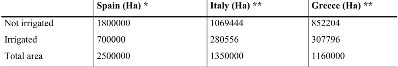
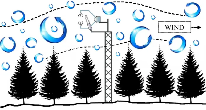
Figure 2.1: Simple graphical representation of turbulent flux in a forest ecosystem. Figure 2.2: Graphical representation of flux footprint.

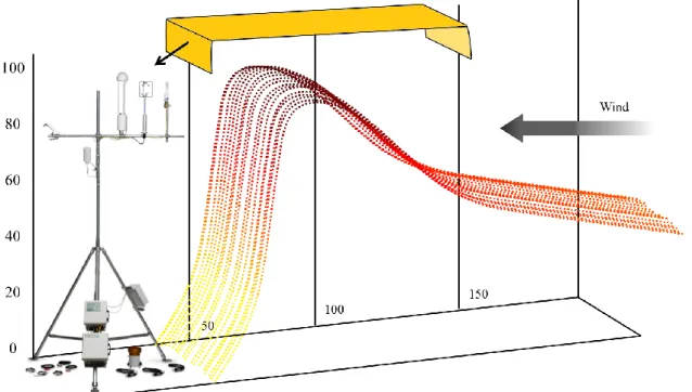
Figure 2.3: Simple scheme of energy balance.

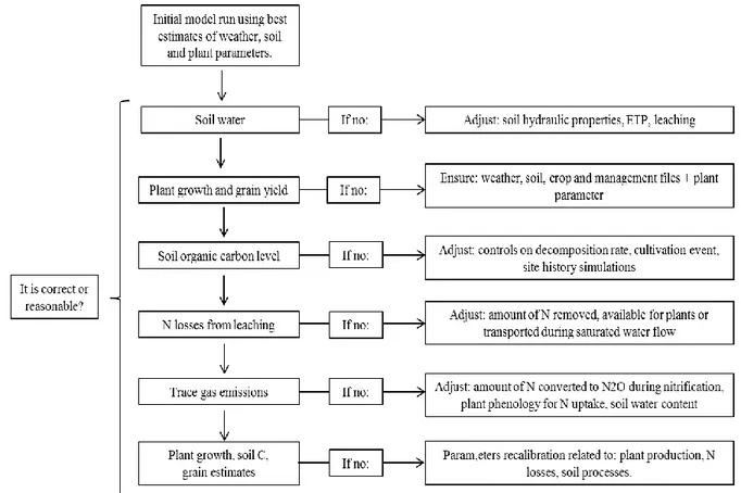
Figure 2.4: Conceptual diagram of the Daycent ecosystem model, Del Grosso et al. (2008). Figure 2.5: Conceptual diagram of the check of Daycent outputs.

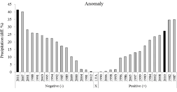
Figure 3.1: Rainfall variability range for the period 1981-2012.

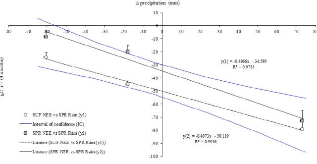
Figure 3.2: Correlation between SP NEE and SP Δ rainfall and between SMP NEE and SP Δ rainfall during the 3 years of study.

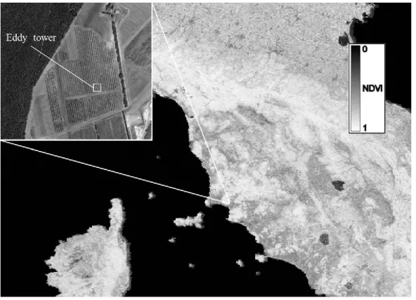
Figure 4.1: MODIS NDVI image of June 2010 showing the position of the study area in Tuscany as well as its main features (enlarged box). NDVI window extends over 8-13° East Longitude, 42-45° North Latitude.

Figure 4.2: Thermo-pluviometric diagram for study area. All monthly data derive from eddy covariance station.

Figure 4.3: Scheme of the multi-step methodology used to estimate olive grove GPP.

Figure 4.4: NDVI profiles of olive trees and ground vegetation during 2010 and 2011. Filled line = olive; dotted line = ground vegetation.

Figure 4.5: Daily estimated GPP profiles of olive trees and ground vegetation during 2010 and 2011. Filled line = olive; dotted line = ground vegetation.

Figure 4.6: Daily values of GPP estimated by C-Fix model (dotted line) and re-constructed from eddy covariance measurements (filled line). The two black bars on the x axis indicate the periods likely affected by the tillages (see text for details).

Figure 4.7: Daily values of GPP estimated by C-Fix model (dotted line) and re-constructed from eddy covariance measurements (filled line). The GPP after the two tillages has been estimated by considering simulated ground vegetation NDVI values (see text for details). Figure 5.1: Model calibration reported at daily time step.

Figure 5.2: Model validation reported at daily time step.

Figure 5.3: Average daily NEE reported for the 4 different timeline under A1B scenario. Figure 5.4: Average monthly NEE reported for the 4 different timeline under A1B scenario.

(10)

List of tables

Table 2.1 List of the 7 Mediterranean countries with the highest worldwide production.

Table 2.2 List of irrigated or not irrigated areas over the main European olive oil makers data 2011*; data 2008 **

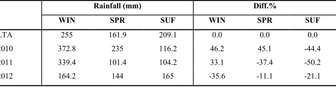
Table 3.1 Monthly meteorological data (i.e. cumulated rainfall, air mean temperature and mean global radiation) of the study area. Data were reported both as long-term average (LTA, 1981-2010) that specifically for the three years of measurements (2010, 2011 and 2012). Table 3.2 Rainfall amount aggregated over 4-months period for the 3 years of study (i.e. 2010, 2011

and 2012) and for LTA. WIN=November, December, January, February; SPR= March, April, May, June; SUF= July, August, September, October.

Table 3.3 Monthly cumulated NEE, GPP and Reco during the three years of measurements.

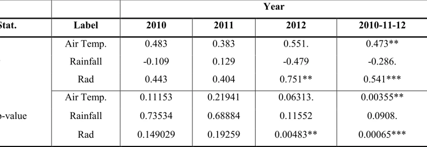
Table 3.4 Correlation between NEE and meteorological variables (air temperature, rainfall and solar radiation) at monthly scale over the three years of study. Signif. codes: 0 ‘***’ 0.001 ‘**’ 0.01 ‘*’ 0.05 ‘.’ 0.1 ‘ ’ 1.

Table 3.5 Correlation between NEE and rainfall aggregated at seasonal scale over the three years of study. SMP=July, August, September, October. SP= March, April, May, June. WP=November, December, January, February. Signif. codes: 0 ‘***’ 0.001 ‘**’ 0.01 ‘*’ 0.05 ‘.’ 0.1 ‘ ’ 1.

Table 4.1: Monthly mean temperature (°C), total rainfall (mm) and months with mean temperature < 0 °C in the study area for 30 years average (MARS JRC data set), 2010 and 2011.

Table 4.2: Number of half-hourly data measured by eddy covariance station in 2010 and 2011. Num.

tot. val. indicates all the measured data; Num. orig. val. indicates all the measured data

used to obtain observed daily GPP data; Num. gaps indicates the measured data that cannot be directly used to obtain observed daily GPP data. For these half-hourly data GPP data were reconstructed using the gap-filling procedure. The quality classification scheme for gap-filled values is: A: best; B: acceptable; C: dubious.

Table 4.3: Accuracy of GPP estimates obtained applying C-Fix model for different time intervals (see text for details on r, RMSE and MBE).

Table 5.1: Soil characteristics of test site. Texture, pH and Bulk density were provided for 4 different soil layers.

Table 5.2: Parameters changed in the file “crop.100” to adjust biomass production for grass layer (Mixed grass from crop default file with 50% warm and 50% cool, N fixation).

(11)

tree from tree default file based on century data).

Table 5.4: Statistical analysis concerning model calibration and validation carried out at different time step.

Table 5.5: Total annual NEE simulated by Daycent model and observed from Eddy Covariance. Total annual NEE was reported considering the same days for observed an simulated.

Table 5.6: Monthly NEE simulated by Daycent model for the baseline and the 3 future timeline under A1B scenario.

(12)

Chapter

1

General Background

Abstract

This chapter gives a general overview about the relationship between agriculture and climate change. Here were indicated the observed and expected climate changes as well as the double role that agricultural systems play in climate change. Main policies and strategies adopted to reduce these changes were also briefly described. Finally, the role of long-term agro ecosystems in climate mitigation has been questioned, focusing the attention especially on the olive orchards.

(13)

Chapter 1. General Background

1.1. Climate change and Agriculture

In the last decades a greater and greater scientific consensus proved that climate change and global warming are a real threat and that they were mostly originated by human-activities. Proofs of changes in climate trends have been provided by several scientific authorities and particularly from IPCC, a scientific intergovernmental body of the United Nations that produces reports aimed at supporting the United Nations Framework Convention on Climate Change (UNFCCC). The latest observations of the atmosphere and surface provided by WGI of AR5-IPCC (IPCC, 2013) indicate that in the last century (1901-2012) almost the entire globe has experienced surface warming (IPCC, 2013). In particular, the global surface temperature (lands and oceans) calculated over the period 1880-2012 showed a warming of 0.85°C (IPCC, 2013). Moreover, it is virtually certain that since 1950 both maximum and minimum averages temperatures are increased. Concerning hydrological cycle and especially precipitation regimes, despite data quality cannot guarantee high levels of confidence, precipitation has been estimated to be increased over northern areas from the beginning of the century. IPCC 2013 also reported that the numbers of cold days and night is decreased while those of warm days and night is increased. Furthermore, heavy precipitation events are increased over several worldwide region, especially Europe and North America (high confidence). Even drought and dryness periods are probably increased since 1970 (low confidence).

Looking at future climate projections for the end of the 21st century with respect to a baseline period of 1986–2005, climate trends are expected to worsening significantly with a general strongest warming comprises between 0.3 and 4.8 °C depending on the concentration-driven RCPs applied (IPCC, 2013). Focusing on Europe, Kjellström et al. (2011) indicated that the strongest warming will be observed during summer especially over Southern Europe, whilst it will be expected in wintertime in Northern Europe. They also indicated a precipitation increase in Northern Europe and a strong decrease in Southern Europe. Concerning extremes, Lenderink and Van Meijgaard, (2008) indicated a very likely increase in heat waves, droughts and heavy precipitation events over the whole Europe. These changes in climate are expected to be particularly detrimental for agriculture. Agricultural sector, indeed, is characterized by a complex two-way relationship with climate. From one hand, crop growth is highly sensitive to change in temperature and precipitations since these factors can cause modification in phenology

(14)

that can bring at decrease of crop yield and increases in cultivation cost (Chmielewski et al., 2004; Seguin et al., 2007; Olesen et al., 2011; Brilli et al., 2014). By contrast, agriculture contributes to global warming through the emissions of greenhouse gases (GHGs) that are originated by the most common agricultural activities such as fertilization, mechanical harvesting, tillage, etc. (Paustian et al., 2004; Smith et al., 2007; IPCC, 2007; Fisher et al., 2012; Bennetzen et al., 2012). Currently, agriculture contributes to 14% of all anthropogenic GHG emissions and to 58% of the world's anthropogenic non-carbon dioxide (CO2) GHG emissions

(Denman et al., 2007; Beach et al., 2008).

1.2. European context: Instruments and Strategies

In the last years several policies and agricultural strategies have been developed with the aim to reduce crop yield losses or limiting the GHG emissions. Despite these measures should be quickly implemented and applied, just few countries have currently developed large-scale programmes to cope with climate change and its associated impacts on crop systems Europe, however, is currently the global area where these programmes were more widely developed and applied (e.g. European Climate Change Programme (ECCP), European Union Emissions Trading System (EU ETS), Renewable Energy Directive, the “20-20-20” Policy, among others).

These programmes in agree with the appointed organisms (e.g. IPCC) have indicated as the best way to cope with climate change those measures for "adaptation" and "mitigation". The first are strategies aimed at reducing economic losses due to crop yield decrease and the high costs of management inputs as fertilizer or irrigation (Smith and Olesen, 2010). These strategies, usually adopted by farmers, mainly consist of changes in cultivar types, sowing date, management, etc. (Bindi and Olesen, 2011). Differently the latter are strategies aimed at reducing GHG emissions from agriculture and, at the same time, at stabilizing the GHG already present in atmosphere, thus minimizing the vulnerability of physical and biophysical systems.

Mitigation strategies are referred both to forestry that agriculture and are mainly based on three aims: i) enhancing removals by increasing of reforestation and carbon sequestration from forest and agricultural soils; ii) reducing emissions by increasing efficiency energy and change in land management; iii) avoiding or displacing emissions through bioenergy production. These aims can be achieved through the application of several practices aimed at increasing C in soil or reducing N emissions (i.e. minimum or no tillage, fertilizer application reduction, energy consumption reduction, grass cover, etc.).

(15)

1.3. Long term agro-ecosystems: role in climate change mitigation

According to Dickie et al. (2014), mitigation potential estimated for agricultural sector can vary from 5.4 to 6.3 Gt CO2eq. This magnitude is mainly due to a combination of three important

factors: emissions reduction, sequestration of carbon in agricultural systems, and major shifts in consumption patterns. Estimates provided by Dickie et al. (2014) indicate that agricultural sector may result roughly GHG neutral. However, whilst the mitigative potential of several crop systems has been analysed, just few studies were focused at evaluating the role of long term agro-ecosystem. The contribution that these systems can provide in mitigation should not be neglected since they can stock large amount of C in woody compartments and soils. Moreover, the cultivation of these systems is widespread over the most sensitive areas to climate change such as Mediterranean basin. Despite according to IPCC, (2013) “tree cover and biomass in long term agro ecosystem (e.g. fruit orchard or savanna) has increased over the past century” (Angassa and Oba, 2008; Witt et al., 2009; Lunt et al., 2010; Rohde and Hoffman, 2012), thus enhancing carbon storage per hectare (Hughes et al., 2006; Liao et al., 2006; Throop and Archer, 2008; Boutton et al., 2009), there is still an open issue: how much do we really know about the mitigation capacity provided by these systems?

In order to solve this question, it is needed to know the prevailing ecological usage of the term "savanna". Savannas systems are complex ecosystems usually structured in two different layers (grass and trees) in which contrasting plant life forms co-dominate (Scholes and Archer, 1997). These systems are widely extensive especially over tropical and temperate regions where they result to be very economically important since involved in fruit production. They are usually assessed and categorized based on several parameters such as stature, canopy cover, and arrangement of woody elements (Sarmiento, 1984; Johnson and Tothill, 1985; Cole, 1986; Burgess, 1995). According to several studies (Archer et al., 1988; Menaut et al., 1990; Tongway and Ludwig, 1990; San Jose et al., 1991; Montania, 1992) these systems are classified within specific ecoregions: tropical and subtropical savannas; temperate savannas; Mediterranean savannas; flooded savannas and montane savannas.

Around Mediterranean basin, where climate change is expected to be detrimental for agriculture, the most typical tree species into Mediterranean savanna are oaks and olive trees. In particular these latter can be considered the most important fruit tree around the basin. This specie has high agronomic and economic value besides at providing a multitude of ecosystem services.

(16)

Based on these premises the main aim of this work was assessing the role that a typical Mediterranean olive orchard can play in climate change mitigation. This aim was reached through a mid-term study (3 years) carried out at Follonica (Tuscany, central Italy), in which eddy covariance measurements allowed the assessment of the C-sequestration capacity as well as the evaluation of C-fluxes dynamics in respect of the main meteorological variables or management practices.

Processed eddy covariance data were additionally used to calibrate and validate two different models which resulted to be able at simulating gross primary production (GPP) and the net ecosystem exchange (NEE) of our test site. Doing so, we implemented new tools able to predict changes in mitigation capacity that savanna systems such as olive orchard will encounter in the next decades, or at developing and evaluating new mitigation strategies based on the changed climatic conditions.

(17)

Chapter

2

Materials and methods

Abstract

Chapter 2 is divided into 3 sections: section 2.1 explores the fruit tree species (i.e. Olea Europaea, L.) that has been studied. This section discusses about taxonomic framework and the characteristics of the specie, phenology, eco-physiology and C-fluxes, as well as the economic importance both at local and worldwide. Section 2.2 describes the eddy covariance method. The major part of information presented in this section make reference to the book “Eddy Covariance Method for Scientific, Industrial, Agricultural and Regulatory Applications” by George Burba. This section is intended to provide the physical and mathematical principles, the major sources of errors and data processing of the eddy covariance method. Finally, section 2.3 explores mathematical models, especially more deeply analysing those remote sensing and biogeochemical models that were used in this thesis.

(18)

Chapter 2. Materials and methods

2.1. Olive tree

2.1.1. Taxonomic framework

The olive tree (Olea europaea L.) is a fruit tree belonged to Oleaceae family. Some authors insert Oleaceae family within the Scrophulariales order (12 families and more than 12000 species), while others authors insert it in an itself order, called Oleales. Although Oleaceae family have a regular tetramera corolla and only two stamens, these latter should be considered modifications occurred from the reduction of the typical flower (which has a pentamer corolla ), therefore it would not have to be inserted in another taxon nor considered more archaic than the rest of the order. The Oleaceae family is composed of 24 genera, consisting of approximately 600 species. Among these, more than half belong to Jasminum genus, very important as it includes species of considerable economic importance such as Olea europea. The family consists of trees and shrubs, characterized by mostly opposite leaves , simple or compound (Grossoni, 1997). Flowers are usually complete, commonly grouped into inflorescences. Corolla consists of 4 petals. The form of fruit is variable, ranging from "Samara" (i.e. Fraxinus L.) to "capsule" (Syringa L.), or "berry" (Ligustrum L.), until most-known "drupe" (Phillyrea L. and Olea L.).

2.1.2. Geographical range

Olive tree is a typical Mediterranean specie which extends from the Iberian Peninsula to Anatolia, including coastal areas of Italy and North Africa. Although olive trees cultivation is currently widespread around the whole Mediterranean basin, the original area of this specie can be considered the Caucasus (Syria and Palestine), where the first farming communities began a systematic selection of different varieties. The olive trees cultivation was for long time exclusive of Mediterranean countries due to the favourable climate conditions. In the last years, however, olive tree cultivation has been spread in many other countries with similar climate conditions such as California, Australia, Argentina and South Africa. Olive trees systems are placed on the marginal land that are unsuitable for intensive cultivation due to soil type, topography, lack of water for irrigation, etc., therefore the major part of the traditional orchards are formed by widely spaced trees. The very old origin of this specie in conjunction with the longevity of individual trees and the continuative use of vegetative propagation, allowed the development of a wide numbers of cultivars. According to Connor et al. (2005), whilst in Spain, Greece, and Tunisia, a

(19)

small numbers of cultivars dominate intensive production areas, in Italy there is more variation between the several cultivation areas. In Italy, the cultivation area of olive tree correspond to Lauretum. The specie prefers temperate climates, ranging from areas characterized by warm and dry summers (evergreen sclerophyllous Mediterranean) to cooler areas until 500-600 m above sea level, while, on the contrary it avoids foggy areas with cold temperatures in winter. The best areas for growth is central and southern Italy, including islands and other areas where climate is tempered by the presence of large bodies of water such as lakes (i.e. Lombardy and Veneto).

2.1.3. Botanic description

Olive tree under free growth conditions can reach 10 meters in height, but it does not exceeds 4-5 meters. It is a long-lived plant that, under favourable conditions, can live more than thousand years. The canopy have a rounded shape (oval, enlarged, lax) but it can change based on pruning and variety. Trunk is irregular and twisted, with the presence of ribs or cords, tending to divide itself forming some cavity. The wood is hard and heavy. The bark is characterized by a grey-ash colour that does not change along the entire life. Olive tree can easily regenerate itself from the stump thanks to several globular structures (i.e. spheroblasts or ovules) that yearly provide many basal shoots. Leaves are simple, elliptical, leathery and shortly “petiolate” with the entire margin. They are green at the top of the page with the other side silvery-grey. This latter can vary depending on species and age. Flowers are hermaphrodite, with a small persistent calyx for 4 deciduous teeth and a tubular corolla with 4 lobes long white 1 cm. Flowers are usually inflorescences (10-15) that are produced from the axils of the leaves of the branches of the previous year. Flowering duration is different for individual trees (i.e. 10 days) and orchards (i.e. from 20 to 30 days). Pollen production lasts for about 5 days while individual stigmas remain receptive for about 2 days. Wind is the main driver of pollen production. This eco-physiological process is very delicate since it is hindered by strong or hot winds, intense rainfall and high temperatures. Orchards with an average pollen production are able to guarantee the reproductive success. By contrast, the reproductive success for individual trees is strictly connected to the number of flower and pollen produced.

2.1.4. Phenology

Olive tree is a day-neutral plant. Fruit production begins when the specie has 3/4 years, whilst the full production after 8 years. Complete maturity is reached after about 20 years. Production

(20)

of nodes, the expansion of leaves and the thickening of stems (i.e. vegetative growth) occur at any time during the year. Vegetative growth is constrained by specific meteorological parameters such as solar radiation, low temperature in winter, and water availability during summer. Typical Mediterranean orchards (i.e. rainfed orchards) show two different peaks of vegetative growth, in spring and autumn, respectively (Connor, 2005). The phenological cycle of olive tree consists of several stages characterized by different level of sensitive to climatic conditions. During winter, the vernalization process (or dormancy) happens when trees are exposed to cooler temperatures (<7ºC). This process leads to the second phase of the reproductive process (i.e. the initiation of induced buds). The length of this phase depends on meteorological conditions (i.e. length of cold time). Then, the vegetative growth starts in February/March, when the lateral and apical buds begin to grow and stretch, showing the issuance of new vegetation that is clearly recognizable by the colour of the new buds. During this period the vegetative growth is mainly driven by the increase of temperature. Vegetative growth is characterized by the growth of shoots and buds. This physiological phase ends around the middle of the Spring, when both shoots and buds reach their final dimensions. The growth of fruits and seeds can lead to the floral induction inhibition, thus contributing to the alternate bearing. This characteristic is particularly clear observing the pattern of biennial flowering and yield. More specifically, years with intense fruiting are usually followed by years with restricted flowering. Although this pattern is very common in almost all fruit trees, olive tree is the fruit tree mostly representative, however (Rallo, 1998). Floral induction occurs in mid-summer (7 to 8 weeks after full bloom) around the time of pit hardening (endocarp hardening). The bloom is characterized by a very high number of flowers. Flowers dropping is considerable and it takes the name of "colatura". The transition from flower to fruit is defined as Fruit Set and usually occurs at the end of June. At this stage corolla enlarges and dries out, persisting until the enlarged ovary causes the detachment. During this phase many factors such as the sudden lowering and remarkable of the temperature, water stress and warm winds can have a negative impact on the percentage of Fruit Set. During the next 4/5 months, olives develop and grown. This long period, which consists of 3 distinguishable sub-phases, ends around November when the fruit has reached the final dimensions. The first sub-step is characterized by the increase (until 20%) of the drupes. Then the hardening of the heart is observed in conjunction with a decrease of fruits growth. The drupes reach the 50% of their final dimensions while the core becomes hard. This sub-step lasts until the end of August. Finally, fruits growth vary based on the climate elapse. In rainfed orchards the olives growth and oil

(21)

content are mainly driven by summer rains, especially those between August and September. Drought conditions can lead to small fruit size and low oil yield. On the contrary, autumnal rainfalls increase the size of the olives, but do not influence the olive oil yield. The olives ripening takes place between October and December, depending to the variety and geographical location. Ripening phase is characterized by the change of colour of the olives. This change is gradual, from green to straw yellow, up to purplish red. It usually includes at least 50% of the surface of the drupe. This period takes the name of veraison and it is characterized by a strong scalar component both among different varieties and intra-variety. Olives range from 1 to 6 grams and their size, shape and colour vary based on the different varieties. During veraison the olive oil content increases while the pulp becomes more soft. Olives reach the complete maturity before the plant ends its growing cycle.

2.1.5. Ecophysiology

Crop growth and productivity are mostly determined by intrinsic characteristics of the specie and climatic conditions of the site. Crop growth, however, is also determined by soil characteristics (physical-chemical structure, morphology, texture, etc.) and management (tillages, fertilization, pruning, etc.). The interactions involving the relation plant-environment are very complex. These interactions affect the plants at physiological and biochemical level, causing different response in terms of development and productivity. Understanding these interactions in olive trees is complex due to physiological characteristics of this specie since it has characterized by a particular reproductive cycle and alternate bearing (Fiorino, 2001). Olive tree is a typically thermophile species with strong xerophil characters. The spontaneous subspecies of olive tree (wild olive tree) is found in degraded spots, scrublands and rocky vegetation, coastlines, etc. The specie is characterized by high grazing resistance, taking on a bushy habit with dense and thorny branching. Olive tree has a remarkable ability to re-grow vigorous suckers from the stump after fires, while is sensitive to low temperatures. The specie suffers shading. When it is found under shadow conditions produces few branches, little canopy and low flowering. The climatic factor determining for olive trees distribution is temperature. The first signs of suffering are clear at temperatures of 3-4 ° C, below these temperatures the tips of the shoots wither. The cold sensitivity increases from the stump to branches. Frosts can cause the death of the entire tree, but the most critical damages appear when temperatures are stable for longer time below -5/6 ° C. According to long term studies carried out in California by Hartmann’s group (Denney and

(22)

McEachern, 1983) the optimum temperature regime for olive tree flowering is in a range from 2 to 4ºC (minima) and from 15.5 to 19ºC (maximum). Water stress is the main parameter affecting production, especially in warm environments such as many areas of Mediterranean. In particular flowering and fruit growth are the most critical periods during the whole vegetative cycle. In these stages water stress (both lower or stronger) reduces the percentage of fruit set, leading to a fruit drop and causing the ripening during summer with a consequent low percentage of olive oil production. Olive tree, however, even in dry areas can provide a minimal level of production. Harmful climatic factors are also strong wind , especially when associated with low temperature, excessive rainfall and elevated air humidity. This specie does not requires specific soils, preferring however loose soil and medium texture, fresh and well drained. Optimal soil conditions for growth are also coarse soils or shallow with outcropping rocks. On the contrary, it suffers heavy soils and subject to stagnation. The dynamics of roots growth is still little known. Olive tree root systems can be extended until the edge of canopy projection. They are also superficial, with root length density (RLD, cm/cm-3) that can be less than in herbaceous crops and some deciduous orchards (Fereres and Goldhamer, 1990). Roots are mostly shallow and temporary. The 70% of roots is found in the first 50-60 cm. Palese et al. (2000) in a study aimed at evaluating the seasonal distribution of olive root growth in southern Italy, observed that they tend to be concentrated within the wetted volume. Maximum root length density is usually observed in winter-spring under rainfed conditions, and during summer under irrigation (Connor, 2005). Olive tree is also one of the fruit tree species that can better tolerate high level of salinity, thus resulting suitable for cultivation close to coastlines.

2.1.6. C-exchanges

Olive tree is a C3 specie with high rate of photorespiration. The major photosynthesis limitations

are high temperatures and light intensity as well as high level of CO2 concentration. Concerning

the plant compartments, leaves are the main element involved in gas exchanges. This is due to the abundance of persistent elements which regulate in- and out-fluxes from leaves. The net photosynthesis rate is not much high, reaching the maximum just for short periods and under specific physical-chemical conditions (i.e. high organic N content in leaves, optimal temperature, high soil water content, etc.). The photosynthetic rate, on average, usually varies with the changes of environmental and varietal conditions. The highest photosynthesis values are usually recorded during the morning, followed by a gradual decrease during the hottest hours

(23)

(afternoon). The photosynthetic activity can be observed also within fruits, especially in the early stages of development whilst it is reduced during veraison. The assimilation rate changes even according to temperature values. It decreases with temperatures higher than 35 °C and lower than 5-7 °C due to the considerable increase of plant respiration. On the contrary, the specie finds the highest assimilation rate in a range between 25 and 28 °C. Although this specie can tolerate high level of water stress, it is highly influenced by the levels of light. Therefore, olive tree is very vulnerable to photoinhibition when water deficit happens in conjunction with excess of light.

2.1.7. Economy and statistics

Although olive tree is a typical Mediterranean species and its cultivation has always been widespread around the whole basin, in the last 30 years its cultivation has also been extended in others countries such as California, Australia, Argentina and South Africa. The spreading of olive tree cultivation in these countries was due to the interaction between favourable climate conditions for the growth of the specie with new type of feeding required. Nowadays, the area involved in olive tree cultivation consists of about 9 million 200 thousand hectares around the world (FAO, 2009) with overwhelmingly development (over 98%) in countries bordering the Mediterranean basin. This is confirmed by data from FAOSTAT (FAOSTAT, 2013), which indicate that more than 85% of the area cultivated with olive trees and 52% of worldwide production comes from 7 Mediterranean countries (i.e. Greece, Italy, Spain, Tunisia, Morocco, Syria and Turkey) (Tab. 2.1).

Country Area Harvested (Ha) Production (tonnes) % (Ha) % (tonnes)

World 9661531.8 18294357.44 100.00 100.00 Greece 820304.8 1123772 8.49 6.14 Italy 1173406 1591104 12.15 8.7 Morocco 615362.6 641002.6 6.37 3.5 Spain 2412106 3146124 24.97 17.2 Syria 637039.4 616001.8 6.59 3.37 Tunisia 1853830 1673430 19.19 9.15 Turkey 766020 842231.4 7.93 4.6 Total 8278068.8 9633665.8 85.68 52.66

(24)

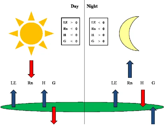
Moreover, according to Vossen, (2007) this area consists of over 700 million olive trees thus representing the almost all of global areas where this specie is cultivated. Available data for 2010 indicate that the EU area involved in olive tree cultivation covers about 5 million hectares and the higher concentration is found in Spain (50%), Italy (26%) and Greece (22%). The higher production of fruits is mainly observed in southerly regions (Andalusia, Calabria, Apulia, Crete and the Peloponnese) due to the high drought tolerance of the specie. Infact the major part of olive orchards it's not irrigated (Tab. 2.2). For instance in Spain more than 80% of the production is concentrated in Andalusia, a region characterized by a predominance of non-irrigated olive trees, although there is an increase of irrigated areas. Its cultivation is usually placed in disadvantaged areas (i.e. mountain areas) covering until 88% of the total area of olive groves in Portugal, 71% in Greece, 60% in Spain and 51% in Italy. Latest data from FAO confirmed that the average production of olive oil in European Union was around 2.2 million tons, representing approximately 73% of world production. Spain , Italy and Greece accounted for roughly 97 % of the production of olive oil EU, of which 62% from Spain. From the point of view of quality, the production of the three types of olive oil (extra virgin, virgin, and lamp) showed differences in percentage between Spain and Italy. In particular Spain provided 35%, 32% and 33% of extra virgin, virgin oil, and lamp oil respectively, while in Italy the same categories have represented respectively 59% , 18% and 24 %. The percentages ranging from one year to another due to differences in meteorological conditions.

Spain (Ha) * Italy (Ha) ** Greece (Ha) **

Not irrigated 1800000 1069444 852204

Irrigated 700000 280556 307796

Total area 2500000 1350000 1160000

Table 2.2 - List of irrigated or not irrigated areas over the main European olive oil makers. data 2011*; data 2008 **

In 2009/10 the global consumption was about 2839000 tons, representing a situation of substantial stability among the major consumer areas (E.U and the United States) of which 65% (about 1856000 tons) in EU and 9% (about 260000 tons ) in U.S. (AGEA and Italian olive oil consortium , 2010). Among the new consumers interesting data come from Australia ( about 37000 tons) and Russia (about 18000 tons, while within the UE the greater demand come from Italy (38 %) Spain (30%) and Greece (12%) (AGEA, 2010). Concerning the international trade

(25)

Italy can be considered both as net importer than exporter of olive products . The foreign trade of olive oil is the greatest and it involves importation (over 500000 tons in the last four years) of which the main required products are extra virgin and virgin (73%). In 2009 were imported 517300 tons for a total value of 1.3 billion euro, while exportation involved 336210 tons and 1.2 billion euro (ISTAT 2010). The main foreign olive oil imported by Italy in the last four years was from Spain ( 52%), Greece ( 19%) and Tunisia (20 %). Exports is more or less constant , especially in terms of volume and especially thanks to the required of the U.S market . Improvements have occurred in Italian exports to France (+10%) and UK (+16% ) (ISTAT 2010). Concerning Italy in the last forty years the agricultural area covered by olive orchards has increased more than 3 times compared to the previous years, especially considering that in 1967 was less of 3 million of hectares. In Italy the area covered by this cultivation is very wide (18 regions out of 20), and the only areas in which the specie is not commonly cultivated are mountains and Po valley due to winter low temperatures and the presence of fog and rime. According to the data released by the Italian Ministry of Agriculture (MIPAAF, 2010), about 18 million of olive trees are grown in Italy on 1350000 ha of land (about 165 trees/ha). Traditional plots are usually small, averaging less than one hectare at national level. Crop production average is around 3000 kg/ha or 16 kg/tree and is mainly concentrated in southern regions such as Apulia (32.25%), Calabria (30.31%) and Sicily (9.42%) (AGEA, 2010). Concerning Tuscany, olive trees occupy an area of 56000 hectares, corresponding to 15 % of the UAA . The major part of olive tree cultivation is found in hilly areas (68.3%), extending to the north (Lunigiana and Garfagnana) and in central and southern areas (Chianti, Val d’Orcia, Val d'Era, Val di Cecina). The remaining fraction (32%) involves mountainous areas (24%) and Maremma plains (8%). The world production for the year 2009 was 2.8 million tons (AGEA and Italian olive oil consortium, 2010).

(26)

2.2. Eddy Covariance Method

The information presented in this section make reference to the book “Eddy Covariance Method for Scientific, Industrial, Agricultural and Regulatory Applications” by George Burba (Burba, 2013). This section is intended to provide the physical and mathematical principles, the major sources of errors and data processing of the eddy covariance method.

2.2.1. State of methodology

In the last 70 years human activities have strongly contributed to rising atmospheric carbon dioxide concentration (CO2). The effect of CO2 increases on terrestrial ecosystems was widely

studied since the beginning of the century, when Browne and Escombe (1902) performed the first plant growth experiments. Following, several instruments were developed and applied to understand the influence of CO2 (ambient and elevated) on plant growth. However instruments

such as Plant Growth Chambers, Leaf Chambers or Greenhouses open-top field Chambers did not provide very reliable results. This was due to two main issues: firstly, the alteration of the studied environment; secondly, the large number of replicas needed for having a statistically reliable measure. These issues were overcame through the development and application of the micrometeorological technique Eddy Covariance (E.C). In recent years this technique has established itself as an alternative method for the quantitative assessment of C exchanges at ecosystem scale (Baldocchi and Meyers, 1988; Baldocchi et al., 1996; Running et al., 1999; Canadell et al., 2000; Baldocchi, 2003; Valentini, 2003). It allows continuous measurements within the test site and it does not disturb the environment above the canopies. Moreover, it is relatively independent from morphology and meteorological conditions (Wesely, 1970). E.C allows to measure the turbulent fluxes exchanged between canopy and atmosphere (Stull, 1988). This technique takes in account movements of air particles (eddies) which are developed above the canopy, in conjunction with the mass of gases transported by the motion itself. The technique is based on a simple principles: the net sequestration of carbon dioxide provided by an ecosystem is calculated as the difference between the C entering and leaving from the system (Wesely, 1970). Fluxes can be counted at different time-scale (from half-hour to seasonal) (Stull, 1988). The measures obtained can also concern heat and water fluxes, methane and trace gases. The technique is also used for calibrating climate models on different spatial-scale (medium and global scale) as well as ecological models able to show dynamics of biogeochemical cycles. These measures are also used for validating data from remote sensing or aircraft (Stull, 1988).

(27)

Currently, different methods, approaches, and numerous network (i.e. Fluxnet, Ameriflux, CarboEurope, FluxNet Canada, Icos, etc.) provide information with high accuracy about fluxes exchanged between several ecosystems (i.e. forests, long-term agro-ecosystems, crop systems, etc.) and atmosphere. Mostly applications have been developed on vegetation, but aerial experiences on board modified aircraft (Sky Arrow) and boas (usually limited by rainfall and gyroscopic effects) are currently increasing. The two main elements needed for the E.C technique application are the three-dimensional ultrasonic anemometer and the infra-red gas analyser (IRGA). The first detects the wind speed in its three spatial components (x, y, z), while the second measures the concentration of carbon dioxide and water vapor in the atmosphere. They work at high frequency, usually comprised between 10 and 20 Hz. Simultaneously to fluxes measures, ancillary measurements should be collected. In particular these measures concern net and global radiation, the air and soil temperature, precipitation amount and humidity. These data are necessary for understanding the response of fluxes based on meteorological parameters but also for improving data elaboration (i.e. gap-filling and flux partitioning). Although the E.C. methodology is difficult to unify, in the last years many efforts have been done to consolidate the terminology and provide a general standardization of processing steps (Lee et al., 2004). However, since the experimental sites are usually focused on different purposes, different treatments are often required.

2.2.2. Physical and mathematical principles

The air flux can be imagined as an horizontal flow consisting of several rotating eddies having 3-D components and vertical movement. The eddies responsible for the transport of most of the flux depend on their proximity to the ground. Smaller eddies can be more probably observed close to the ground and they are characterized by fast rotation as well as by higher frequency movements of air. On the contrary larger eddies can be more easily observed away from the ground. They are slower and characterized by lower frequency movements of air the movements of eddies can take from few seconds (or less) until some hours. The Eddy Covariance technique is mainly based on the theory of fluid dynamics, which was applied to the atmosphere by Reynolds (Reynolds, 1886) for the first time. Reynolds has correlated the atmospheric turbulence theory with principles and laws of fluid dynamics, high-lightening how the turbulent fluxes, in addition to the momentum (vector quantity which is able to measure the body's capacity to change the movement of other bodies in which it dynamically interacts), carries the heat and

(28)

other scalar quantities. The equation of conservation of a scalar is the theoretical basis of the Eddy Covariance's technique.

Eq 1. Equation of a scalar conservation. I: temporal variation of the concentration of a C scalar at a given point in space ; II: local advection ; III: average horizontal and vertical divergence (or convergence) of turbulent flux; IV: molecular diffusion ; V: processes of formation (or destruction ) of the molecules related to the considered scalar.

This mathematical formula can be used for an infinitesimal air volume in which “C” is the mixing ratio of a generic scalar, whilst “u”, “v” and “w” correspond to the three components of the wind velocity. The term “D” represents the molecular diffusion process while “Sc” summarizes the processes of formation/destruction of scalar molecules. Vertical bar on the different variables indicates their average over time, while the peak on the variables in III denotes the instantaneous fluctuation of the value from the mean.

The average value obtained between the instantaneous fluctuations of two variables represents the statistics covariance. The covariance between the three wind speed components and the scalar concentration represents the turbulent flux along the three spatial directions (x , y and z). The technique is based on the principle that the vertical flux of an entity on a surface turbulence layer is directly proportional to the covariance of the vertical velocity and to the concentration of that entity. Therefore it allows to measure the sensitivity of the eco-systemic processes which regulate the absorption of carbon dioxide and water vapour at short (hourly based ) and long-term (seasonal or annual ) (Lee et al., 2004). In a more simple way, flux can be defined as an amount of a particle that passes through a closed surface (i.e. a Gaussian) per unit of time (Wyngaard, 1990). In very simple terms, flux describes how much of an entity moves through a unit area per unit time (Swinbank, 1951).

Flux is dependent on:

1) the number of particles which cross an area 2) the size of the crossed area

(29)

As reported in the figure 2.1, flux can be imagined as a stream consisting of several eddies, each one consisting of three spatial components (x, y, z), including the air vertical movement (Kaimal and Finnigan, 1994).

Figure 2.1. – Simple graphical representation of turbulent flux in a forest ecosystem.

For improving the understanding about how the vertical flux can be derived from the covariance between the vertical wind velocity and the concentration of the entity of interest, a simple example was reported: in a time "x", three molecules of CO2 receive a boost upwards while in

the next moment only two molecules of CO2 go down, the net flux at that time correspond to one

molecule of CO2 directed upwards (Baldocchi, 2005). Therefore eddy covariance is based on

assessment of the vertical wind flux by measuring the number of molecules in motion and how fast they continuously ascend and descend. Very sophisticated instruments are necessary to measure the turbulent flux, since the molecular fluctuations occur very quickly. Moreover the variations of molecular concentration, air density and temperature are very small, so needing of very quick and specify calculations.

(30)

In turbulent flow, vertical flux can be presented as:

Eq. 2. Vertical flux in turbulent flow. Flux is equal to a mean product of air density (ρα), vertical wind speed (W), and the dry mole fraction (S) of the gas of interest. The dry mole fraction is often called the mixing ratio.

Reynolds decomposition can be used to indicate means and deviations from the previous equation (Eq.2). Air density has represented as a sum of a mean over some time and an instantaneous deviation from this mean. A similar procedure can be reported also for vertical wind speed and dry mole fraction of the entity of interest.

Eq. 3. Reynolds decomposition of the vertical flux in turbulent flow.

In the third step the flux equation is simplified as showed below:

Eq. 4. Simplified equation of Reynolds decomposition of the vertical flux in turbulent flow.

Two important assumptions have to be made in the conventional eddy covariance method (Lee et al., 2004). First, the air density fluctuations that in case of strong winds may be non-negligible in comparison with the gas flux, in the major part of the cases (i.e. over reasonably flat and vast spaces such as fields or plains) they can be assumed to be negligible. Secondly, the mean vertical flux is assumed to be negligible for horizontal homogeneous terrain, so that no flow diversions or conversions occur (Massman and Lee, 2002). By assuming to be negligible both flux diversion and conversions, the flux becomes equal to the product of the mean air density and the mean covariance between instantaneous deviations in vertical wind speed and mixing ratio, and the classical equation for eddy flux is:

(31)

Besides the turbulent flux, there are other fundamental formulas which allow to better understand the fluxes dynamics on ecosystems. In particular they concern: sensible heat, water vapour and latent heat (Eq. 6-7-8). Sensible heat flux is equal to the mean air density multiplied by the covariance between deviations in instantaneous vertical wind speed and temperature. Including the specific heat term within the equation, it is possible the conversion to energy units.

Eq. 6. Sensible heat flux

Depending on the units of fast water vapor content do exist several representation of water vapor equation. Water vapor is a fundamental parameter for the calculation of turbulent fluxes and it is often computed in energy units (W m-2).

Equazione 7. Traditional water vapor flux.

Latent heat flux describes the energy used in the process of evaporation, transpiration, or evapotranspiration and therefore its values can be converted into other commonly used units such as mm d-1, inches ha-1, kg m-2 h-1, etc..

Eq. 8. Latent heat flux

2.2.3. Flux footprint

Flux footprint is defined as the area mainly covered by the instrument on the tower. More in detail, it is referred to the area upwind from the tower where the major part of the fluxes generated are recorded by the instruments (Fig. 2.2). The concept of flux footprint is essential for proper planning and execution of an eddy covariance experiment. The mostly contribution does not come from extremes (i.e. underneath the tower or many kilometres away), but rather from

(32)

somewhere in between. The right distance to calculate the main area providing the most part of the contributions has to take in account the dependence of the flux footprint on

a) measurement height, b) surface roughness, c) thermal stability.

Figure 2.2. – Graphical representation of flux footprint. Modified from Burba et al. 2013.

Measurement height

Footprint strongly increases:

 at 1.5 m over 80% of the ET came from within 80 m upwind  at 4.5 m over 80% of the ET came from within 450 m upwind Footprint near the station may also be strongly affected:

 at 1.5 m, the area 5 m around the instrument did not affect ET  at 4.5 m, the area 32 m around the instrument did not affect ET

(33)

Surface roughness

Footprint decreases with increased roughness:  at a sensor height of 1.5 m:

 for rough surface over 80% of the ET came from within 80 m upwind  for smooth surface 80% of ET came from about 250 m upwind Footprint near the station is also affected by roughness:

 for rough surface, area 5 m around the instrument did not affect ET  for smooth surface, area 10 m around the instrument did not affect ET

Thermal stability

Thermal stability can increase the footprint size several times:

 For a measurement height of 1.5 m and a canopy height of 0.6 m:  in very unstable conditions, most of the footprint is within 50 m  in neutral conditions, it is within 250 m

 in very stable conditions, footprint is within 500 m

Flux data under very stable conditions need to be corrected or discarded due to insufficient fetch. Flux data at very unstable conditions may need to be corrected or discarded due to the fact that large portion of the flux may come from the disturbed area around the instrument tower.

a. Flux footprint depends on: - Measurement height - Surface roughness - Thermal stability

b. Size of footprint increases with: - Increased measurement height - Decreased surface roughness

- Change in stability from unstable to stable c. Area near instrument tower mostly contribute if:

- Measurement height is low - Surface roughness is high - Conditions are very unstable

(34)

Models able to calculate the flux footprint require specific parameters (i.e. type of instruments, height of the tower (m)of the canopy and eddy tower, wind speed, etc.). these parameters are needed for assessing the area where fluxes are originated and the contribution produced by this area compared to the total footprint. Under normal conditions the contribution of normalized cumulative flux is calculated in terms of percentage according to Eq. 9 (Swuepp et al., 1990).

Eq. 9. Normalized cumulative flux

2.2.4. Processing eddy covariance

Processing of eddy covariance data can change depending on the methodology adopted by researchers. Methodology can change according to the site-specific design as well the sampling conditions. The major steps include the conversion of the signals from voltages to physical units, despiking, the application of calibration coefficients if needed, rotation of coordinates, correction for time delay, de-trending (if needed), average of fast data over 0.5 to 4 hour periods, the application of frequency response, sonic and density corrections, the quality control, filling of missing periods and integration of long-term flux data. Below are reported three main methods to assess the quality of dataset:

 Raw data assessment  Stationary test

 Test on turbulence and its characteristics

Concerning the validation of eddy data, one of the main methods to evaluate their reliability is building of site-study energy balance. In Fig. 2.3 a simple scheme of energy balance has been reported.

(35)

Figure 2.3 – Simple scheme of energy balance

The energy balance is represented by the follow equation:

Rn: net radiation; L: latent heat; H: sensible heat; G: ground heat or the storage of energy.

Validation using study-site energy balance is simple but functional. Sum of all these components must be equal to 0 to have a perfect closure of the balance. If this happens, all energy transfers have been correctly measured (Rosset et al.,1997). Although a good measure of latent heat doesn't mean a correct measure of CO2 fluxes, correct values observed in latent heat can be taken

as a positive-check about the probably good quality of C fluxes. However, by using eddy covariance the closure of energy balance may be incomplete due to the presence of secondary fluxes which can't be measured with this technique. The optimal closure of the energy balance is represented by the following equation:

(36)

Eddy covariance instruments measure fluxes over the canopy. During periods without atmospheric turbulence (e.g. night-time) these fluxes accumulate under canopies, reducing data reliability. The total contribution of these measures is fundamental to improve the evaluation of NEE in a certain ecosystem.

2.2.5. Gap-filling and flux-partitioning

A better understanding of ecosystem dynamics can be reached by separating the net ecosystem exchange (NEE) as the gross primary production (GPP) and ecosystem respiration (Reco) through an algorithm to partition the flow (flux partitioning). This method allows to improve the knowledge on the assimilators or breathings processes that are often poorly represented (Falge et al., 2002a; Reichstein et al., 2002b). Flux partitioning also improve the understanding of inter-annual variability of NEE and its dependence by climate or other parameters (Valentini et al., 2000). Before the application of the flux partitioning algorithm, a previous step is necessary. This step, called gap-filling, consists of filling the data gaps that occur in adverse weather conditions or in the event of failure to tools to estimate the long-term budgets.

These processes were following briefly described.

a. Gap-filling

The gap-filling method is built on the co-variation of the fluxes with meteorological variables (air temperature, radiation and vapour of pressure deficit, VPD) and the temporal auto-correlation of the fluxes. On the basis of the gap type (i.e. length of the period, available meteorological parameters, etc.), missing data are substituted by values obtained on the basis of data measured in similar meteorological conditions within a time window of ± 7-14 days. Otherwise, missing data can be exchanged with values obtained on the basis of data measured in the same time of the day.

b. Flux partitioning

Flux partitioning algorithm allows to estimate Reco and Gross Primary Productivity (GPP) from NEE according to the definition equation:

(37)

Different methods to separate the net ecosystem exchange (NEE) into its major components (i.e. GPP and Reco) have been developed. The algorithms can use (filtered) night-time data for the estimation of ecosystem respiration, daytime data or both day- and night-time data, using light-response curves.

The most applied algorithm has been described by Reichstein et al. 2005 and consist of a regression model. Flux-partitioning uses raw data (not gap-filled) to derive Reco from the relation between temperature and nocturnal NEE, which represents the solely the respiratory process. The method proposed by Reichstein et al. (2005) refers to that developed by Lloyd and Taylor, (1994) (Eq. 11):

Eq. 11. Ecosystem respiration equation from the method proposed by Lloyd and Taylor, (1994); T: air temperature; T0: is a constant 46.02; E0: the activation energy (it determines the temperature sensitivity and is a free parameter); Tref: set to 10°C.

Since Reco is a parameter that temporally varies in an ecosystem, Reichstein et al. (2005) used the nonlinear regression model by Lloyd and Taylor (1994) fixing all parameters with the only exception of 'Reco,ref'. They estimated this parameter just once using the long-term temperature sensitivity and another by the short-term temperature sensitivity. Thus, the 'Reco,ref' estimates were assigned to that point in time. Finally the 'Reco,ref' parameters were estimated for each period and linearly interpolated between the estimates, resulting as a dense time series of parameters. Consequently, for each point in time, Reichstein et al. (2005) provided Reco estimates according to the following equation:

Eq. 12. Ecosystem respiration equation from the method proposed by Reichstein et al. (2005); T: air temperature; T0: is kept constant at 46.02 as in Lloyd & Taylor (1994);E0: the activation energy (it determines the temperature sensitivity and is a free parameter); Tref: is set to 10°C as in the original model; (T): time-dependent parameters and variables.

(38)

2.3. Simulation models

Simulation is defined as the process able to imitate instantaneous or long-term processes of a system. Simulation can provide useful information concerning the assessment of the system’s characteristics, the main elements that can affect it, and elements needed for its development. The ability to reproduce a certain system or process allows comparisons with similar systems, resulting in benefits such as an optimal parameterization, critical issues and possibility to predict future performances. Simulations can provide advantages such as possibility to test things or strategies before to apply them, time reduction, understanding of systems dynamics, exploration of new policies and managements, diagnostic, etc.. However simulations have two main problems: the first one is due to the cost for building or implementing the tools, the second is the difficulty to understand and interpret results obtained. In the last 30 years, crop simulation models are became fundamental tools for scientific research and planning of agro-systems. The spreading of these tools is due to their easy application in several environment and under different conditions (i.e. management, climate, variety) compared to those in which they have been developed. In addition, while ground based measurements are limited at small spatial and temporal scales (e.g. gas concentration) due to snapshots of state variables, the models can offer full spatial and temporal coverage (Del Grosso et al., 2008). In this work were used two different kind of models. The first one is a remote sensing model called C-fix that was described and applied in paper 2. The second is a biogeochemical model called Daycent, described and applied in paper 3.

a. Remote sensing models:

Remote sensing is a technology that involves specific electromagnetic sensors usually installed over satellite or aircraft to measure and monitor changes in the earth's surface and atmosphere (Showengerdt, 2006). In recent years remote sensing models have been widely applied to assess crop growth and yield estimation, thus resulting as the best source of data for large scale applications and study. This methodology is mainly based on satellite images which give a series of numbers resulting as the amount of the energy reflected from the earth's surface in different wavelength bands. Among the different bands, the major part of information concerning vegetation growth and physiological conditions can be found into the infrared bands, that are not visible to the human eye. Infact the majority of approaches using remote sensing for monitoring and managing both natural and crop systems involves dissimilarity in reflectance properties

(39)

between visible and NIR wavelengths (Knipling, 1970; Bauer, 1975). Green leaves show lower values for reflectance and transmittance within visible regions of the spectrum (i.e., 400 to 700 nm) but higher in the near-infrared regions (NIR, 700 to 1300 nm) (Bouman, 1992). One of the main advantages using satellite images is the possibility to observe many times changes in surface conditions. For instance, given that a satellite regularly passes over the same land, it become possible to continuously catch new data about land use as well as monitoring physiological conditions over the year. Remotely-sensed images are also usually combined with ground observations to obtain a complete picture of changes. For instance one of the most simple method for extracting the green plant quantity signal is the vegetation indices (VGT). This indices are computed as differences, ratios, or linear combinations of reflected light in visible and NIR wavebands (Tucker, 1979; Jackson, 1983). Vegetation indices such as the ratio vegetation index (RVI _ NIR/Red) and normalized difference vegetation index NDVI _ (NIR _ Red)/(NIR 1 Red) are optimal for investigating biomass measures through the season since they are well correlated with green biomass and leaf area index of crop canopies (Pinter et al., 2003).

b. Biogeochemical models:

Biogeochemical or biogeochemistry (BGC) models are able to reproduce several ecosystemic processes concerning both plant physiology that entity exchanges. These models therefore can explain vegetation phases such as growth, competition, senescence and mortality but also processes related to natural energy and matter exchanges (i.e. H2O, C, N) between vegetation,

soil and the atmosphere. The major part of these models is mainly based on climate conditions, soil characteristics, nutrient and water supply. Although these tools can represent whole systems and their interaction with other components (i.e. biosphere, atmosphere, hydrosphere), they can be divided according to specific characteristics to deal with soil processes, agricultural crops or forestry only. They can be used also to simulate external effects such as the impact of current and future climate change on crop growth, the effect of different management on soil carbon and water balances, and many others. These tools can represent the behaviour of plant growth functions and exchange processes through mathematical equations. The main physiological processes (e.g. crop growth) are usually correlated with the most important meteorological parameters such as temperature, radiation and rainfall (water and nutrient supply). BGC models can vary also depending on their scale of investigation. For instance some models can be applied to a single plant or vegetation type while other can be used over large areas if representative of